Appendix A. Summary Measurements, Time Spent Within Thresholds, and Analysis of ICP/AMP/RAP
The following appendix contains the tables for summary measurements and percentage of time spent within certain thresholds, across the whole population. All the significant p-values were marked bold.
AMP, pulse amplitude of ICP; CPP, cerebral perfusion pressure; CT, computed tomography; GOSE, Glasgow outcome scale-extended; ICP, intracranial pressure; MAP, mean arterial blood pressure; PRx, pressure reactivity index; RAP, compensatory reserve index; std, standard deviation.
Table A1.
Summary measurements.
Table A1.
Summary measurements.
| Metrics | ICP | MAP | CPP | AMP | RAP |
|---|
| mean | 10.818 | 85.374 | 74.555 | 2.244 | 0.632 |
| std | 7.564 | 13.881 | 14.049 | 1.855 | 0.483 |
| min | −15 | 0.035 | −34.26 | 0 | −1 |
| 25% | 6.138 | 76.69 | 66.5005 | 0.9977 | 0.49635 |
| 50% | 10.17 | 83.94 | 73.03 | 1.711 | 0.8578 |
| 75% | 14.74 | 92.65 | 81.69 | 2.91 | 0.9646 |
| max | 80.06 | 200 | 197.362 | 22.41 | 1 |
Table A2.
Time spent within threshold.
Table A2.
Time spent within threshold.
| Ranges | Time Spent (Unit) | % Time Spent | Total Time (Unit) |
|---|
| [0.4, 1] | 267.578 | 78.091 | 342.646 |
| (0, 0.4) | 30.889 | 9.014 |
| [0, −1] | 43.166 | 12.597 |
Table A3.
Sub-group analysis—age (first comparison).
Table A3.
Sub-group analysis—age (first comparison).
| Condition | ICP | MAP | CPP | AMP | RAP |
|---|
Below 40 years
(n = 46) | 10.56481 ± 6.85241 | 84.44187 ± 7.36121 | 73.68225 ± 7.94464 | 1.71982 ± 1.21450 | 0.60043 ± 0.18153 |
Above 40 years
(n = 63) | 8.51253 ± 6.63832 | 84.07349 ± 7.70570 | 76.12142 ± 8.49570 | 2.40335 ± 1.82718 | 0.53754 ± 0.20982 |
| p-value | 0.047852 | 0.710493 | 0.136793 | 0.065227 | 0.119867 |
Table A4.
Sub-group analysis—age (second comparison).
Table A4.
Sub-group analysis—age (second comparison).
| Condition | ICP | MAP | CPP | AMP | RAP |
|---|
Below 40 years
(n = 46) | 10.56481 ± 6.85241 | 84.44187 ± 7.36121 | 73.68225 ± 7.94464 | 1.71982 ± 1.21450 | 0.60043 ± 0.18153 |
Between 40 and 60 years
(n = 39) | 8.71919 ± 7.12835 | 86.03822 ± 8.03764 | 77.66581 ± 9.36177 | 2.21371 ± 1.61825 | 0.59274 ± 0.19015 |
Above 60 years
(n = 24) | 8.17672 ± 5.88620 | 80.88080 ± 6.01193 | 73.61179 ± 6.25669 | 2.71151 ± 2.12438 | 0.44784 ± 0.21301 |
| p-value | 0.28399 | 0.02818 | 0.05323 | 0.04624 | 0.00459 |
Table A5.
Sub-group analysis—M/F Sex.
Table A5.
Sub-group analysis—M/F Sex.
| Condition | ICP | MAP | CPP | AMP | RAP |
|---|
| Male (n = 89) | 8.90705 ± 6.30729 | 84.74958 ± 7.90121 | 76.15799 ± 8.24657 | 2.02947 ± 1.54173 | 0.55111 ± 0.20298 |
| Female (n = 20) | 11.47718 ± 8.42448 | 81.91215 ± 5.12074 | 70.34861 ± 7.02543 | 2.49502 ± 1.96119 | 0.62181 ± 0.17918 |
| p-value | 0.333628 | 0.192417 | 0.00805 | 0.483515 | 0.164657 |
Table A6.
Sub-group analysis—pupillary response.
Table A6.
Sub-group analysis—pupillary response.
| Condition | ICP | MAP | CPP | AMP | RAP |
|---|
Bilat Reactive
(n = 65) | 9.68200 ± 6.32553 | 84.11428 ± 7.34526 | 74.95088 ± 7.44597 | 2.25631 ± 1.76652 | 0.59983 ± 0.19003 |
Bilat Unreactive
(n = 19) | 7.21860 ± 6.62510 | 85.25445 ± 10.43550 | 77.67136 ± 10.39840 | 1.84440 ± 1.38851 | 0.51583 ± 0.19264 |
Unilateral Unreactive
(n = 25) | 10.23149 ± 7.88851 | 83.74773 ± 5.33723 | 73.49879 ± 8.63051 | 1.95276 ± 1.41453 | 0.50780 ± 0.21717 |
| p-value | 0.29519 | 0.79378 | 0.25327 | 0.53557 | 0.07446 |
Table A7.
Sub-group analysis—Marshall CT grade.
Table A7.
Sub-group analysis—Marshall CT grade.
| Condition | ICP | MAP | CPP | AMP | RAP |
|---|
| Grade II (n = 3) | 8.41885 ± 1.46502 | 88.19054 ± 2.95348 | 79.67350 ± 4.20626 | 1.10567 ± 0.32360 | 0.53874 ± 0.23926 |
| Grade III (n = 31) | 10.10747 ± 5.75164 | 85.77724 ± 7.99221 | 75.28605 ± 6.88824 | 2.34405 ± 1.30344 | 0.65335 ± 0.16089 |
| Grade IV (n = 20) | 13.85727 ± 7.61941 | 86.37602 ± 7.24507 | 73.34250 ± 8.89201 | 3.30238 ± 2.28233 | 0.67305 ± 0.16134 |
| Grade V (n = 55) | 7.39158 ± 6.41152 | 82.35945 ± 7.18358 | 75.36899 ± 9.00899 | 1.60895 ± 1.28146 | 0.47552 ± 0.19312 |
| p-value | 0.00227 | 0.06480 | 0.60516 | 0.00028 | 0.00001 |
Table A8.
Sub-group analysis—alive/dead (1-month GOSE).
Table A8.
Sub-group analysis—alive/dead (1-month GOSE).
| Condition | ICP | MAP | CPP | AMP | RAP |
|---|
| Alive (n = 71) | 8.08183 ± 5.20270 | 84.54202 ± 7.87658 | 76.48282 ± 8.44677 | 1.65068 ± 1.01478 | 0.57072 ± 0.19835 |
| Dead (n = 38) | 11.98871 ± 8.45046 | 83.68252 ± 7.01954 | 72.27488 ± 7.38769 | 2.96776 ± 2.15609 | 0.55279 ± 0.20754 |
| p-value | 0.033485 | 0.668784 | 0.031911 | 0.002865 | 0.604539 |
Table A9.
Sub-group analysis—favorable/unfavorable (1-month GOSE).
Table A9.
Sub-group analysis—favorable/unfavorable (1-month GOSE).
| Condition | ICP | MAP | CPP | AMP | RAP |
|---|
| Favourable (n = 52) | 7.29237 ± 5.30263 | 84.20479 ± 7.90128 | 77.03737 ± 8.74621 | 1.44024 ± 0.79148 | 0.54361 ± 0.20245 |
| Unfavorable (n = 57) | 11.46599 ± 7.36347 | 84.27194 ± 7.30886 | 73.11250 ± 7.46122 | 2.73982 ± 1.94607 | 0.58373 ± 0.19920 |
| p-value | 0.001883 | 1.0 | 0.016348 | 0.000358 | 0.294478 |
Table A10.
Sub-group analysis—alive/dead (6-month GOSE).
Table A10.
Sub-group analysis—alive/dead (6-month GOSE).
| Condition | ICP | MAP | CPP | AMP | RAP |
|---|
| Alive (n = 68) | 8.42374 ± 5.18191 | 84.72952 ± 7.98240 | 76.32846 ± 8.45665 | 1.66250 ± 1.02750 | 0.58264 ± 0.19200 |
| Dead (n = 41) | 11.37039 ± 8.47379 | 83.53319 ± 7.27248 | 72.68237 ± 7.72236 | 2.83479 ± 2.12879 | 0.53877 ± 0.21121 |
| p-value | 0.169741 | 0.562849 | 0.065448 | 0.010051 | 0.258864 |
Table A11.
Sub-group analysis—favorable/unfavorable (6-month GOSE).
Table A11.
Sub-group analysis—favorable/unfavorable (6-month GOSE).
| Condition | ICP | MAP | CPP | AMP | RAP |
|---|
| Favourable (n = 25) | 8.12572 ± 5.14666 | 84.64676 ± 8.09823 | 76.55841 ± 8.59283 | 1.67795 ± 1.04272 | 0.57845 ± 0.19602 |
| Unfavorable (n = 64) | 11.61034 ± 8.23577 | 83.83620 ± 6.72062 | 72.72268 ± 7.47357 | 2.77978 ± 2.10187 | 0.54720 ± 0.20960 |
| p-value | 0.048501 | 0.738688 | 0.041701 | 0.01456 | 0.4034 |
Table A12.
ICP thresholds.
Table A12.
ICP thresholds.
| Condition | ICP | MAP | CPP | AMP | RAP |
|---|
| ICP > 22 | 28.34662 ± 7.12649 | 91.16469 ± 17.08712 | 62.81109 ± 17.58897 | 4.99916 ± 3.26314 | 0.72418 ± 0.43710 |
| ICP < 20 | 9.34625 ± 5.61682 | 84.79938 ± 13.48051 | 75.54584 ± 13.34231 | 2.06319 ± 1.57050 | 0.62705 ± 0.48596 |
| p-value | Close to 0 | Close to 0 | Close to 0 | Close to 0 | Close to 0 |
Table A13.
AMP thresholds.
Table A13.
AMP thresholds.
| Condition | ICP | MAP | CPP | AMP | RAP |
|---|
| AMP < 1 | 6.99299 ± 5.69411 | 84.26304 ± 14.03507 | 77.38008 ± 13.74575 | 0.58311 ± 0.26164 | 0.43376 ± 0.55036 |
| 1 < AMP < 3 | 10.94096 ± 7.58453 | 85.39152 ± 13.89387 | 74.56503 ± 14.06739 | 2.31228 ± 1.93635 | 0.63582 ± 0.48283 |
| AMP > 3 | 15.60541 ± 8.33541 | 86.79509 ± 14.63808 | 71.22871 ± 14.81692 | 5.01951 ± 1.90360 | 0.78769 ± 0.36104 |
| p-value | Close to 0 | Close to 0 | Close to 0 | Close to 0 | Close to 0 |
Table A14.
PRx thresholds (first comparison).
Table A14.
PRx thresholds (first comparison).
| Condition | ICP | MAP | CPP | AMP | RAP | PRx |
|---|
| PRx < 0 | 10.44394 ± 6.53201 | 85.41019 ± 12.90041 | 74.88617 ± 12.82014 | 2.22166 ± 1.73685 | 0.68340 ± 0.44809 | −0.42581 ± 0.26188 |
| PRx > 0 | 11.25437 ± 8.56936 | 85.55157 ± 14.99946 | 74.20460 ± 15.28773 | 2.27123 ± 1.98214 | 0.57066 ± 0.51977 | 0.42869 ± 0.27811 |
| p-value | Close to 0 | Close to 0 | Close to 0 | Close to 0 | Close to 0 | Close to 0 |
Table A15.
PRx thresholds (second comparison).
Table A15.
PRx thresholds (second comparison).
| Condition | ICP | MAP | CPP | AMP | RAP | PRx |
|---|
| PRx < 0.25 | 10.82641 ± 7.57303 | 85.47692 ± 13.93089 | 74.56473 ± 14.04217 | 2.24505 ± 1.85682 | 0.63016 ± 0.48653 | −0.02201 ± 0.50469 |
| PRx > 0.25 | 11.77002 ± 9.13674 | 85.55960 ± 15.74818 | 73.67751 ± 16.11601 | 2.34873 ± 2.09150 | 0.55701 ± 0.52997 | 0.57686 ± 0.21250 |
| p-value | Close to 0 | Close to 0 | Close to 0 | 0.002642 | Close to 0 | Close to 0 |
Appendix B. Stationarity Test Analysis—ADF/KPSS Tests for Original and Differenced Data
The following are specific p-values for stationary tests at the minute-by-minute resolution, confirming that, for the most part, the data were stationary after the first ordered differencing for both ADF and KPSS tests.
ADF, Augmented Dickey–Fuller; AMP, pulse amplitude of ICP; ICP, intracranial pressure; KPSS, Kwiatkowski–Phillips–Schmidt–Shin; RAP, compensatory reserve index.
Table A16.
ADF test p-values for original data at the minute-by-minute resolution.
Table A16.
ADF test p-values for original data at the minute-by-minute resolution.
| Patient | ICP | AMP | RAP |
|---|
| TBI_001 | close to 0 | close to 0 | close to 0 |
| TBI_002 | close to 0 | close to 0 | close to 0 |
| TBI_003 | 0.01 | 0.16 | close to 0 |
| TBI_004 | close to 0 | close to 0 | close to 0 |
| TBI_007 | 0.02 | 0.59 | close to 0 |
| TBI_008 | 0.33 | close to 0 | close to 0 |
| TBI_009 | close to 0 | 0.08 | close to 0 |
| TBI_010 | close to 0 | 0.01 | close to 0 |
| TBI_011 | close to 0 | close to 0 | close to 0 |
| TBI_012 | close to 0 | close to 0 | close to 0 |
| TBI_013 | 0.19 | 0.14 | close to 0 |
| TBI_014 | 0.98 | 0.72 | close to 0 |
| TBI_015 | close to 0 | close to 0 | close to 0 |
| TBI_016 | 0.04 | 0.01 | close to 0 |
| TBI_017 | 0.03 | 0.09 | close to 0 |
| TBI_018 | 0.55 | 0.17 | close to 0 |
| TBI_019 | 0.47 | 0.25 | 0.03 |
| TBI_020 | close to 0 | close to 0 | close to 0 |
| TBI_021 | 0.58 | 0.22 | close to 0 |
| TBI_022 | 0.02 | 0.02 | close to 0 |
| TBI_023 | close to 0 | close to 0 | close to 0 |
| TBI_024 | close to 0 | close to 0 | close to 0 |
| TBI_025 | 0.26 | 0.27 | close to 0 |
| TBI_026 | close to 0 | close to 0 | close to 0 |
| TBI_027 | 0.12 | 0.16 | close to 0 |
| TBI_028 | close to 0 | close to 0 | close to 0 |
| TBI_029 | close to 0 | close to 0 | close to 0 |
| TBI_030 | close to 0 | close to 0 | close to 0 |
| TBI_031 | 0.1 | 0.04 | close to 0 |
| TBI_032 | 0.23 | 0.05 | close to 0 |
| TBI_033 | close to 0 | close to 0 | close to 0 |
| TBI_034 | 0.01 | 0.01 | close to 0 |
| TBI_036 | close to 0 | close to 0 | close to 0 |
| TBI_037 | close to 0 | close to 0 | close to 0 |
| TBI_038 | close to 0 | close to 0 | close to 0 |
| TBI_039 | close to 0 | close to 0 | close to 0 |
| TBI_040 | close to 0 | 0.02 | close to 0 |
| TBI_041 | close to 0 | close to 0 | close to 0 |
| TBI_042 | close to 0 | close to 0 | close to 0 |
| TBI_043 | close to 0 | close to 0 | close to 0 |
| TBI_044 | 0.03 | 0.1 | close to 0 |
| TBI_045 | close to 0 | close to 0 | close to 0 |
| TBI_046 | close to 0 | close to 0 | close to 0 |
| TBI_047 | close to 0 | 0.14 | close to 0 |
| TBI_048 | 0.54 | 0.63 | close to 0 |
| TBI_049 | close to 0 | close to 0 | close to 0 |
| TBI_050 | close to 0 | close to 0 | close to 0 |
| TBI_051 | 0.33 | 0.42 | close to 0 |
| TBI_052 | 0.68 | 0.12 | close to 0 |
| TBI_053 | 0.01 | 0.01 | close to 0 |
| TBI_054 | 0.05 | 0.01 | close to 0 |
| TBI_055 | close to 0 | close to 0 | close to 0 |
| TBI_056 | 0 | close to 0 | close to 0 |
| TBI_057 | close to 0 | close to 0 | close to 0 |
| TBI_058 | 0 | close to 0 | close to 0 |
| TBI_059 | 0.06 | 0.05 | close to 0 |
| TBI_060 | close to 0 | close to 0 | close to 0 |
| TBI_061 | close to 0 | 0.08 | close to 0 |
| TBI_062 | 0.01 | 0.27 | close to 0 |
| TBI_063 | close to 0 | 0.01 | close to 0 |
| TBI_064 | 0 | 0.42 | close to 0 |
| TBI_065 | 0.03 | 0.04 | close to 0 |
| TBI_066 | 0 | close to 0 | close to 0 |
| TBI_067 | close to 0 | close to 0 | close to 0 |
| TBI_068 | 0 | 0.12 | close to 0 |
| TBI_069 | close to 0 | close to 0 | close to 0 |
| TBI_070 | 0.42 | 0.99 | close to 0 |
| TBI_071 | close to 0 | close to 0 | close to 0 |
| TBI_072 | 0.05 | 0.37 | close to 0 |
| TBI_073 | close to 0 | close to 0 | close to 0 |
| TBI_074 | close to 0 | close to 0 | close to 0 |
| TBI_075 | close to 0 | close to 0 | close to 0 |
| TBI_076 | close to 0 | close to 0 | close to 0 |
| TBI_077 | close to 0 | close to 0 | close to 0 |
| TBI_078 | close to 0 | 0.28 | close to 0 |
| TBI_079 | 0.49 | close to 0 | close to 0 |
| TBI_080 | close to 0 | close to 0 | close to 0 |
| TBI_081 | close to 0 | close to 0 | close to 0 |
| TBI_082 | 0.72 | 0.17 | close to 0 |
| TBI_083 | 0.02 | 0.06 | close to 0 |
| TBI_084 | 0.05 | 0.06 | close to 0 |
| TBI_085 | close to 0 | close to 0 | close to 0 |
| TBI_086 | close to 0 | close to 0 | close to 0 |
| TBI_087 | 0.01 | 0.06 | close to 0 |
| TBI_088 | close to 0 | close to 0 | close to 0 |
| TBI_089 | close to 0 | close to 0 | close to 0 |
| TBI_090 | 0 | 0.01 | close to 0 |
| TBI_091 | close to 0 | close to 0 | close to 0 |
| TBI_092 | close to 0 | close to 0 | close to 0 |
| TBI_093 | close to 0 | close to 0 | close to 0 |
| TBI_094 | 0.57 | close to 0 | close to 0 |
| TBI_095 | close to 0 | close to 0 | close to 0 |
| TBI_096 | 0.29 | close to 0 | close to 0 |
| TBI_097 | 0.02 | 0.04 | close to 0 |
| TBI_098 | close to 0 | 0.01 | close to 0 |
| TBI_099 | close to 0 | close to 0 | close to 0 |
| TBI_100 | close to 0 | close to 0 | close to 0 |
| TBI_101 | 0.55 | close to 0 | close to 0 |
| TBI_102 | 0.02 | 0.2 | close to 0 |
| TBI_103 | close to 0 | close to 0 | close to 0 |
| TBI_104 | close to 0 | close to 0 | close to 0 |
| TBI_105 | 0.04 | close to 0 | close to 0 |
| TBI_106 | close to 0 | close to 0 | close to 0 |
| TBI_107 | 0.1 | close to 0 | close to 0 |
| TBI_108 | close to 0 | close to 0 | close to 0 |
| TBI_109 | 0.01 | close to 0 | close to 0 |
| TBI_110 | close to 0 | close to 0 | close to 0 |
| TBI_111 | close to 0 | close to 0 | close to 0 |
| TBI_112 | 0.07 | close to 0 | close to 0 |
Table A17.
KPSS test p-values for original data at minute-by-minute resolution.
Table A17.
KPSS test p-values for original data at minute-by-minute resolution.
| Patient | ICP | AMP | RAP |
|---|
| TBI_001 | 0.01 | 0.01 | 0.01 |
| TBI_002 | 0.01 | 0.01 | 0.01 |
| TBI_003 | 0.01 | 0.01 | 0.01 |
| TBI_004 | 0.08 | 0.1 | 0.1 |
| TBI_007 | 0.01 | 0.01 | 0.1 |
| TBI_008 | 0.01 | 0.07 | 0.1 |
| TBI_009 | 0.01 | 0.01 | 0.01 |
| TBI_010 | 0.1 | 0.01 | 0.01 |
| TBI_011 | 0.01 | 0.01 | 0.01 |
| TBI_012 | 0.02 | 0.01 | 0.1 |
| TBI_013 | 0.03 | 0.07 | 0.1 |
| TBI_014 | 0.01 | 0.01 | 0.01 |
| TBI_015 | 0.01 | 0.01 | 0.1 |
| TBI_016 | 0.01 | 0.01 | 0.01 |
| TBI_017 | 0.01 | 0.1 | 0.1 |
| TBI_018 | 0.01 | 0.01 | 0.01 |
| TBI_019 | 0.01 | 0.01 | 0.01 |
| TBI_020 | 0.01 | 0.01 | 0.01 |
| TBI_021 | 0.01 | 0.01 | 0.01 |
| TBI_022 | 0.01 | 0.01 | 0.01 |
| TBI_023 | 0.01 | 0.01 | 0.01 |
| TBI_024 | 0.01 | 0.01 | 0.02 |
| TBI_025 | 0.01 | 0.01 | 0.1 |
| TBI_026 | 0.03 | 0.01 | 0.01 |
| TBI_027 | 0.1 | 0.1 | 0.01 |
| TBI_028 | 0.01 | 0.1 | 0.01 |
| TBI_029 | 0.01 | 0.01 | 0.01 |
| TBI_030 | 0.01 | 0.01 | 0.1 |
| TBI_031 | 0.03 | 0.05 | 0.01 |
| TBI_032 | 0.01 | 0.01 | 0.08 |
| TBI_033 | 0.01 | 0.02 | 0.03 |
| TBI_034 | 0.01 | 0.01 | 0.01 |
| TBI_036 | 0.01 | 0.01 | 0.01 |
| TBI_037 | 0.01 | 0.01 | 0.01 |
| TBI_038 | 0.01 | 0.01 | 0.01 |
| TBI_039 | 0.01 | 0.01 | 0.01 |
| TBI_040 | 0.01 | 0.01 | 0.02 |
| TBI_041 | 0.01 | 0.01 | 0.1 |
| TBI_042 | 0.01 | 0.02 | 0.01 |
| TBI_043 | 0.01 | 0.01 | 0.09 |
| TBI_044 | 0.01 | 0.01 | 0.1 |
| TBI_045 | 0.01 | 0.01 | 0.01 |
| TBI_046 | 0.01 | 0.01 | 0.1 |
| TBI_047 | 0.01 | 0.01 | 0.1 |
| TBI_048 | 0.01 | 0.01 | 0.01 |
| TBI_049 | 0.01 | 0.01 | 0.1 |
| TBI_050 | 0.01 | 0.1 | 0.1 |
| TBI_051 | 0.01 | 0.01 | 0.1 |
| TBI_052 | 0.01 | 0.01 | 0.01 |
| TBI_053 | 0.01 | 0.01 | 0.01 |
| TBI_054 | 0.02 | 0.01 | 0.1 |
| TBI_055 | 0.01 | 0.01 | 0.01 |
| TBI_056 | 0.02 | 0.1 | 0.1 |
| TBI_057 | 0.01 | 0.01 | 0.01 |
| TBI_058 | 0.01 | 0.01 | 0.01 |
| TBI_059 | 0.01 | 0.01 | 0.01 |
| TBI_060 | 0.01 | 0.01 | 0.01 |
| TBI_061 | 0.01 | 0.01 | 0.1 |
| TBI_062 | 0.01 | 0.01 | 0.07 |
| TBI_063 | 0.01 | 0.01 | 0.1 |
| TBI_064 | 0.01 | 0.01 | 0.01 |
| TBI_065 | 0.01 | 0.01 | 0.01 |
| TBI_066 | 0.01 | 0.01 | 0.01 |
| TBI_067 | 0.1 | 0.09 | 0.1 |
| TBI_068 | 0.01 | 0.01 | 0.01 |
| TBI_069 | 0.01 | 0.01 | 0.01 |
| TBI_070 | 0.01 | 0.01 | 0.02 |
| TBI_071 | 0.01 | 0.01 | 0.01 |
| TBI_072 | 0.01 | 0.01 | 0.01 |
| TBI_073 | 0.1 | 0.01 | 0.01 |
| TBI_074 | 0.01 | 0.01 | 0.01 |
| TBI_075 | 0.05 | 0.01 | 0.01 |
| TBI_076 | 0.01 | 0.01 | 0.1 |
| TBI_077 | 0.1 | 0.1 | 0.01 |
| TBI_078 | 0.02 | 0.01 | 0.1 |
| TBI_079 | 0.01 | 0.01 | 0.01 |
| TBI_080 | 0.01 | 0.01 | 0.1 |
| TBI_081 | 0.01 | 0.02 | 0.01 |
| TBI_082 | 0.01 | 0.01 | 0.02 |
| TBI_083 | 0.01 | 0.01 | 0.01 |
| TBI_084 | 0.01 | 0.01 | 0.1 |
| TBI_085 | 0.01 | 0.01 | 0.1 |
| TBI_086 | 0.01 | 0.01 | 0.01 |
| TBI_087 | 0.01 | 0.01 | 0.01 |
| TBI_088 | 0.02 | 0.01 | 0.01 |
| TBI_089 | 0.01 | 0.01 | 0.01 |
| TBI_090 | 0.01 | 0.02 | 0.01 |
| TBI_091 | 0.01 | 0.01 | 0.01 |
| TBI_092 | 0.01 | 0.01 | 0.01 |
| TBI_093 | 0.01 | 0.01 | 0.01 |
| TBI_094 | 0.01 | 0.01 | 0.09 |
| TBI_095 | 0.01 | 0.01 | 0.01 |
| TBI_096 | 0.1 | 0.1 | 0.01 |
| TBI_097 | 0.01 | 0.01 | 0.05 |
| TBI_098 | 0.01 | 0.01 | 0.05 |
| TBI_099 | 0.02 | 0.01 | 0.01 |
| TBI_100 | 0.05 | 0.01 | 0.02 |
| TBI_101 | 0.01 | 0.01 | 0.01 |
| TBI_102 | 0.01 | 0.01 | 0.01 |
| TBI_103 | 0.01 | 0.01 | 0.02 |
| TBI_104 | 0.01 | 0.01 | 0.01 |
| TBI_105 | 0.01 | 0.01 | 0.01 |
| TBI_106 | 0.01 | 0.01 | 0.1 |
| TBI_107 | 0.01 | 0.09 | 0.01 |
| TBI_108 | 0.01 | 0.01 | 0.01 |
| TBI_109 | 0.09 | 0.01 | 0.1 |
| TBI_110 | 0.01 | 0.01 | 0.01 |
| TBI_111 | 0.01 | 0.01 | 0.01 |
| TBI_112 | 0.01 | 0.01 | 0.02 |
Table A18.
ADF test p-values for differenced data at minute-by-minute resolution.
Table A18.
ADF test p-values for differenced data at minute-by-minute resolution.
| Patient | ICP | AMP | RAP |
|---|
| TBI_001 | close to 0 | close to 0 | close to 0 |
| TBI_002 | close to 0 | close to 0 | close to 0 |
| TBI_003 | close to 0 | close to 0 | close to 0 |
| TBI_004 | close to 0 | close to 0 | close to 0 |
| TBI_007 | close to 0 | close to 0 | close to 0 |
| TBI_008 | close to 0 | close to 0 | close to 0 |
| TBI_009 | close to 0 | close to 0 | close to 0 |
| TBI_010 | close to 0 | close to 0 | close to 0 |
| TBI_011 | close to 0 | close to 0 | close to 0 |
| TBI_012 | close to 0 | close to 0 | close to 0 |
| TBI_013 | close to 0 | close to 0 | close to 0 |
| TBI_014 | close to 0 | close to 0 | close to 0 |
| TBI_015 | close to 0 | close to 0 | close to 0 |
| TBI_016 | close to 0 | close to 0 | close to 0 |
| TBI_017 | close to 0 | close to 0 | close to 0 |
| TBI_018 | close to 0 | close to 0 | close to 0 |
| TBI_019 | close to 0 | close to 0 | close to 0 |
| TBI_020 | close to 0 | close to 0 | close to 0 |
| TBI_021 | close to 0 | close to 0 | close to 0 |
| TBI_022 | close to 0 | close to 0 | close to 0 |
| TBI_023 | close to 0 | close to 0 | close to 0 |
| TBI_024 | close to 0 | close to 0 | close to 0 |
| TBI_025 | close to 0 | close to 0 | close to 0 |
| TBI_026 | close to 0 | close to 0 | close to 0 |
| TBI_027 | close to 0 | close to 0 | close to 0 |
| TBI_028 | close to 0 | close to 0 | close to 0 |
| TBI_029 | close to 0 | close to 0 | close to 0 |
| TBI_030 | close to 0 | close to 0 | close to 0 |
| TBI_031 | close to 0 | close to 0 | close to 0 |
| TBI_032 | close to 0 | close to 0 | close to 0 |
| TBI_033 | close to 0 | close to 0 | close to 0 |
| TBI_034 | close to 0 | close to 0 | close to 0 |
| TBI_036 | close to 0 | close to 0 | close to 0 |
| TBI_037 | close to 0 | close to 0 | close to 0 |
| TBI_038 | close to 0 | close to 0 | close to 0 |
| TBI_039 | close to 0 | close to 0 | close to 0 |
| TBI_040 | close to 0 | close to 0 | close to 0 |
| TBI_041 | close to 0 | close to 0 | close to 0 |
| TBI_042 | close to 0 | close to 0 | close to 0 |
| TBI_043 | close to 0 | close to 0 | close to 0 |
| TBI_044 | close to 0 | close to 0 | close to 0 |
| TBI_045 | close to 0 | close to 0 | close to 0 |
| TBI_046 | close to 0 | close to 0 | close to 0 |
| TBI_047 | close to 0 | close to 0 | close to 0 |
| TBI_048 | close to 0 | close to 0 | close to 0 |
| TBI_049 | close to 0 | close to 0 | close to 0 |
| TBI_050 | close to 0 | close to 0 | close to 0 |
| TBI_051 | close to 0 | close to 0 | close to 0 |
| TBI_052 | close to 0 | close to 0 | close to 0 |
| TBI_053 | close to 0 | close to 0 | close to 0 |
| TBI_054 | close to 0 | close to 0 | close to 0 |
| TBI_055 | close to 0 | close to 0 | close to 0 |
| TBI_056 | close to 0 | close to 0 | close to 0 |
| TBI_057 | close to 0 | close to 0 | close to 0 |
| TBI_058 | close to 0 | close to 0 | close to 0 |
| TBI_059 | close to 0 | close to 0 | close to 0 |
| TBI_060 | close to 0 | close to 0 | close to 0 |
| TBI_061 | close to 0 | close to 0 | close to 0 |
| TBI_062 | close to 0 | close to 0 | close to 0 |
| TBI_063 | close to 0 | close to 0 | close to 0 |
| TBI_064 | close to 0 | close to 0 | close to 0 |
| TBI_065 | close to 0 | close to 0 | close to 0 |
| TBI_066 | close to 0 | close to 0 | close to 0 |
| TBI_067 | close to 0 | close to 0 | close to 0 |
| TBI_068 | close to 0 | close to 0 | close to 0 |
| TBI_069 | close to 0 | close to 0 | close to 0 |
| TBI_070 | close to 0 | close to 0 | close to 0 |
| TBI_071 | close to 0 | close to 0 | close to 0 |
| TBI_072 | close to 0 | close to 0 | close to 0 |
| TBI_073 | close to 0 | close to 0 | close to 0 |
| TBI_074 | close to 0 | close to 0 | close to 0 |
| TBI_075 | close to 0 | close to 0 | close to 0 |
| TBI_076 | close to 0 | close to 0 | close to 0 |
| TBI_077 | close to 0 | close to 0 | close to 0 |
| TBI_078 | close to 0 | close to 0 | close to 0 |
| TBI_079 | close to 0 | close to 0 | close to 0 |
| TBI_080 | close to 0 | close to 0 | close to 0 |
| TBI_081 | close to 0 | close to 0 | close to 0 |
| TBI_082 | close to 0 | close to 0 | close to 0 |
| TBI_083 | close to 0 | close to 0 | close to 0 |
| TBI_084 | close to 0 | close to 0 | close to 0 |
| TBI_085 | close to 0 | close to 0 | close to 0 |
| TBI_086 | close to 0 | close to 0 | close to 0 |
| TBI_087 | close to 0 | close to 0 | close to 0 |
| TBI_088 | close to 0 | close to 0 | close to 0 |
| TBI_089 | close to 0 | close to 0 | close to 0 |
| TBI_090 | close to 0 | close to 0 | close to 0 |
| TBI_091 | close to 0 | close to 0 | close to 0 |
| TBI_092 | close to 0 | close to 0 | close to 0 |
| TBI_093 | close to 0 | close to 0 | close to 0 |
| TBI_094 | close to 0 | close to 0 | close to 0 |
| TBI_095 | close to 0 | close to 0 | close to 0 |
| TBI_096 | 0.05 | close to 0 | close to 0 |
| TBI_097 | close to 0 | close to 0 | close to 0 |
| TBI_098 | close to 0 | close to 0 | close to 0 |
| TBI_099 | close to 0 | close to 0 | close to 0 |
| TBI_100 | close to 0 | close to 0 | close to 0 |
| TBI_101 | close to 0 | close to 0 | close to 0 |
| TBI_102 | close to 0 | close to 0 | close to 0 |
| TBI_103 | close to 0 | close to 0 | close to 0 |
| TBI_104 | close to 0 | close to 0 | close to 0 |
| TBI_105 | close to 0 | close to 0 | close to 0 |
| TBI_106 | close to 0 | close to 0 | close to 0 |
| TBI_107 | close to 0 | close to 0 | close to 0 |
| TBI_108 | close to 0 | close to 0 | close to 0 |
| TBI_109 | close to 0 | close to 0 | close to 0 |
| TBI_110 | close to 0 | close to 0 | close to 0 |
| TBI_111 | close to 0 | close to 0 | close to 0 |
| TBI_112 | close to 0 | close to 0 | close to 0 |
Table A19.
KPSS test p-values for differenced data at minute-by-minute resolution.
Table A19.
KPSS test p-values for differenced data at minute-by-minute resolution.
| Patient | ICP | AMP | RAP |
|---|
| TBI_001 | 0.1 | 0.1 | 0.1 |
| TBI_002 | 0.1 | 0.1 | 0.1 |
| TBI_003 | 0.1 | 0.1 | 0.1 |
| TBI_004 | 0.1 | 0.1 | 0.06 |
| TBI_007 | 0.1 | 0.1 | 0.1 |
| TBI_008 | 0.1 | 0.1 | 0.1 |
| TBI_009 | 0.1 | 0.1 | 0.1 |
| TBI_010 | 0.1 | 0.1 | 0.1 |
| TBI_011 | 0.1 | 0.1 | 0.1 |
| TBI_012 | 0.1 | 0.1 | 0.1 |
| TBI_013 | 0.1 | 0.1 | 0.1 |
| TBI_014 | 0.09 | 0.1 | 0.1 |
| TBI_015 | 0.1 | 0.1 | 0.1 |
| TBI_016 | 0.1 | 0.1 | 0.1 |
| TBI_017 | 0.1 | 0.1 | 0.1 |
| TBI_018 | 0.1 | 0.1 | 0.1 |
| TBI_019 | 0.1 | 0.1 | 0.1 |
| TBI_020 | 0.1 | 0.1 | 0.1 |
| TBI_021 | 0.1 | 0.1 | 0.1 |
| TBI_022 | 0.1 | 0.1 | 0.1 |
| TBI_023 | 0.1 | 0.1 | 0.1 |
| TBI_024 | 0.1 | 0.1 | 0.1 |
| TBI_025 | 0.1 | 0.1 | 0.1 |
| TBI_026 | 0.1 | 0.1 | 0.1 |
| TBI_027 | 0.1 | 0.1 | 0.1 |
| TBI_028 | 0.1 | 0.1 | 0.1 |
| TBI_029 | 0.1 | 0.1 | 0.1 |
| TBI_030 | 0.1 | 0.1 | 0.1 |
| TBI_031 | 0.1 | 0.1 | 0.1 |
| TBI_032 | 0.1 | 0.1 | 0.1 |
| TBI_033 | 0.1 | 0.1 | 0.1 |
| TBI_034 | 0.1 | 0.1 | 0.1 |
| TBI_036 | 0.1 | 0.1 | 0.1 |
| TBI_037 | 0.1 | 0.1 | 0.1 |
| TBI_038 | 0.1 | 0.1 | 0.1 |
| TBI_039 | 0.1 | 0.1 | 0.1 |
| TBI_040 | 0.1 | 0.1 | 0.1 |
| TBI_041 | 0.1 | 0.1 | 0.1 |
| TBI_042 | 0.1 | 0.1 | 0.1 |
| TBI_043 | 0.1 | 0.1 | 0.1 |
| TBI_044 | 0.1 | 0.1 | 0.1 |
| TBI_045 | 0.1 | 0.1 | 0.1 |
| TBI_046 | 0.1 | 0.1 | 0.1 |
| TBI_047 | 0.1 | 0.1 | 0.1 |
| TBI_048 | 0.1 | 0.1 | 0.1 |
| TBI_049 | 0.1 | 0.1 | 0.1 |
| TBI_050 | 0.1 | 0.1 | 0.1 |
| TBI_051 | 0.1 | 0.1 | 0.1 |
| TBI_052 | 0.1 | 0.1 | 0.1 |
| TBI_053 | 0.1 | 0.1 | 0.1 |
| TBI_054 | 0.1 | 0.1 | 0.1 |
| TBI_055 | 0.1 | 0.1 | 0.1 |
| TBI_056 | 0.1 | 0.1 | 0.1 |
| TBI_057 | 0.1 | 0.1 | 0.1 |
| TBI_058 | 0.1 | 0.1 | 0.1 |
| TBI_059 | 0.1 | 0.1 | 0.1 |
| TBI_060 | 0.1 | 0.1 | 0.1 |
| TBI_061 | 0.1 | 0.1 | 0.1 |
| TBI_062 | 0.1 | 0.1 | 0.1 |
| TBI_063 | 0.1 | 0.1 | 0.1 |
| TBI_064 | 0.1 | 0.1 | 0.1 |
| TBI_065 | 0.1 | 0.1 | 0.1 |
| TBI_066 | 0.1 | 0.1 | 0.05 |
| TBI_067 | 0.1 | 0.1 | 0.1 |
| TBI_068 | 0.1 | 0.1 | 0.1 |
| TBI_069 | 0.1 | 0.1 | 0.1 |
| TBI_070 | 0.1 | 0.04 | 0.1 |
| TBI_071 | 0.1 | 0.1 | 0.1 |
| TBI_072 | 0.1 | 0.1 | 0.1 |
| TBI_073 | 0.1 | 0.1 | 0.1 |
| TBI_074 | 0.1 | 0.1 | 0.1 |
| TBI_075 | 0.1 | 0.1 | 0.1 |
| TBI_076 | 0.1 | 0.1 | 0.1 |
| TBI_077 | 0.1 | 0.1 | 0.1 |
| TBI_078 | 0.1 | 0.1 | 0.1 |
| TBI_079 | 0.1 | 0.1 | 0.1 |
| TBI_080 | 0.1 | 0.1 | 0.1 |
| TBI_081 | 0.1 | 0.1 | 0.1 |
| TBI_082 | 0.1 | 0.1 | 0.1 |
| TBI_083 | 0.1 | 0.1 | 0.1 |
| TBI_084 | 0.1 | 0.1 | 0.1 |
| TBI_085 | 0.1 | 0.1 | 0.1 |
| TBI_086 | 0.1 | 0.1 | 0.1 |
| TBI_087 | 0.1 | 0.1 | 0.1 |
| TBI_088 | 0.1 | 0.1 | 0.1 |
| TBI_089 | 0.1 | 0.1 | 0.1 |
| TBI_090 | 0.1 | 0.1 | 0.1 |
| TBI_091 | 0.1 | 0.1 | 0.1 |
| TBI_092 | 0.1 | 0.1 | 0.1 |
| TBI_093 | 0.1 | 0.1 | 0.1 |
| TBI_094 | 0.1 | 0.1 | 0.1 |
| TBI_095 | 0.1 | 0.1 | 0.1 |
| TBI_096 | 0.1 | 0.1 | 0.1 |
| TBI_097 | 0.1 | 0.1 | 0.1 |
| TBI_098 | 0.1 | 0.1 | 0.1 |
| TBI_099 | 0.1 | 0.1 | 0.1 |
| TBI_100 | 0.1 | 0.1 | 0.1 |
| TBI_101 | 0.1 | 0.1 | 0.1 |
| TBI_102 | 0.1 | 0.1 | 0.1 |
| TBI_103 | 0.1 | 0.1 | 0.1 |
| TBI_104 | 0.1 | 0.1 | 0.1 |
| TBI_105 | 0.1 | 0.1 | 0.1 |
| TBI_106 | 0.1 | 0.1 | 0.1 |
| TBI_107 | 0.1 | 0.1 | 0.1 |
| TBI_108 | 0.1 | 0.1 | 0.1 |
| TBI_109 | 0.1 | 0.1 | 0.1 |
| TBI_110 | 0.1 | 0.1 | 0.1 |
| TBI_111 | 0.1 | 0.1 | 0.1 |
| TBI_112 | 0.1 | 0.1 | 0.1 |
Appendix E. Residuals, ACF, and PACF Plots of Residuals and Analysis
This appendix contains the figures and tables for the evaluation of the median optimal ARIMA models. Included are comparative ACF/PACF plots of the residuals (original vs. post-ARIMA) for a single patient’s ICP and AMP data at both minute-by-minute and hour-by-hour resolutions. Additionally, the variance of the overall data, the residual variance, and the count of significant spikes are provided both for an individual patient and as a summary of the entire population to demonstrate effective data modeling.
ACF, autocorrelative function; AMP, pulse amplitude of ICP; ARIMA, auto-regressive integrated moving average; ICP, intracranial pressure; PACF, partial ACF; RAP, compensatory reserve index.
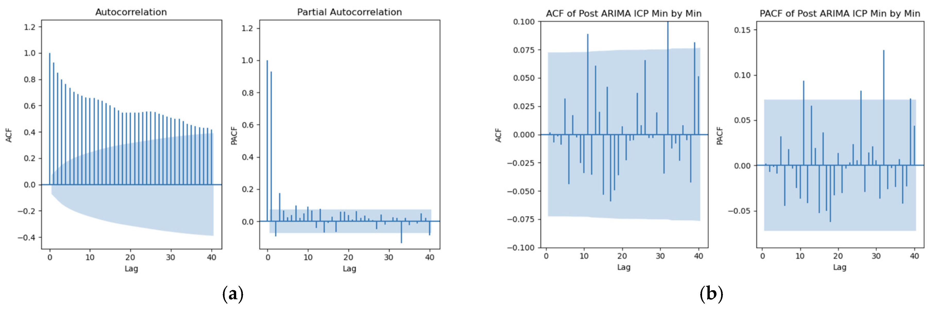
Figure A1.
ACF and PACF plots for ICP at minute-by-minute resolution for an individual. (a) RAP pre-ARIMA plots, (b) RAP post-ARIMA (5, 1, 1) plots.
Figure A1.
ACF and PACF plots for ICP at minute-by-minute resolution for an individual. (a) RAP pre-ARIMA plots, (b) RAP post-ARIMA (5, 1, 1) plots.
The figure corresponds to the ACF and PACF plots of residuals of the ICP signal (a) before and (b) after ARIMA (5, 1, 1), demonstrating that the model moderately accounts for the ICP structure.
Figure A2.
ACF and PACF plots for ICP at different resolutions for an individual. (a) At 10-min-by-10-min resolution with ARIMA (2, 1, 2), (b) at 30-min-by-30-min resolution with ARIMA (2, 1, 2), (c) at hour-by-hour resolution with ARIMA (2, 1, 2).
Figure A2.
ACF and PACF plots for ICP at different resolutions for an individual. (a) At 10-min-by-10-min resolution with ARIMA (2, 1, 2), (b) at 30-min-by-30-min resolution with ARIMA (2, 1, 2), (c) at hour-by-hour resolution with ARIMA (2, 1, 2).
The figure documents the ACF and PACF of the residuals of the ICP-mapped ARIMA structure in the (a) 10-min-by-10-min, (b) 30-min-by-30-min, and (c) hour-by-hour relationships.
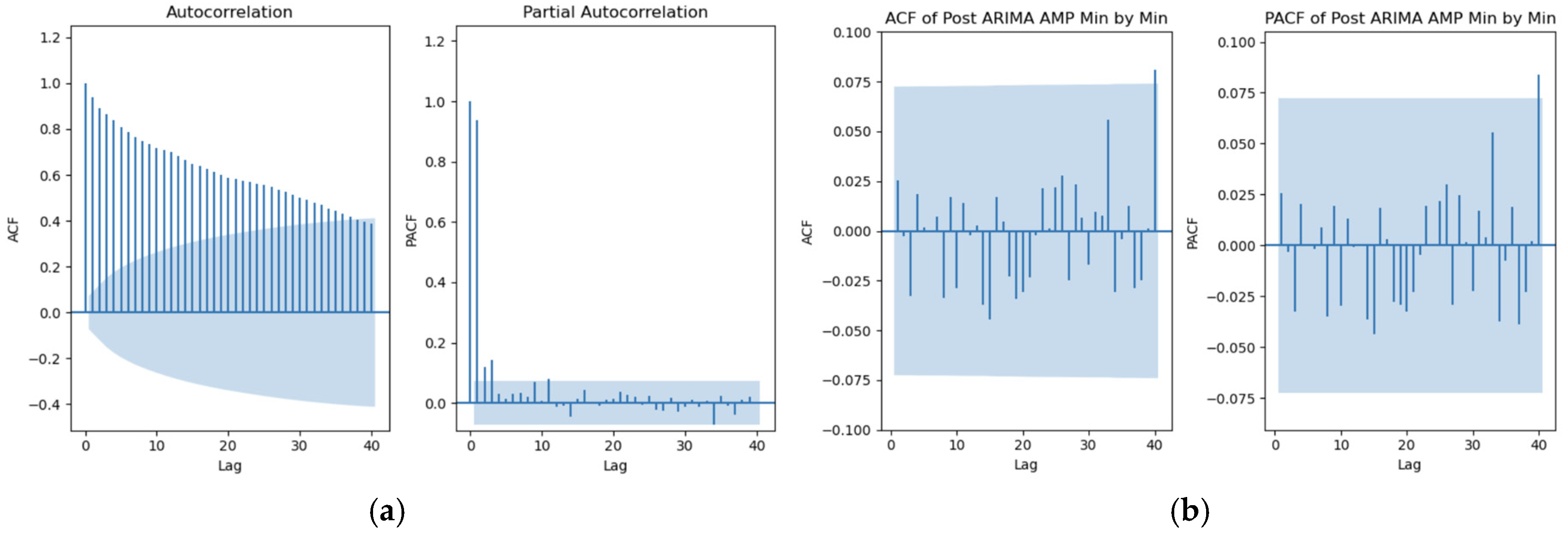
Figure A3.
ACF and PACF plots for AMP at minute-by-minute resolution for an individual. (a) AMP pre-ARIMA plots, (b) AMP post-ARIMA (3, 1, 5) plots.
Figure A3.
ACF and PACF plots for AMP at minute-by-minute resolution for an individual. (a) AMP pre-ARIMA plots, (b) AMP post-ARIMA (3, 1, 5) plots.
The figure corresponds to the ACF and PACF plots of residuals of the AMP signal (a) before and (b) after ARIMA (3, 1, 5), demonstrating that the model moderately accounts for the AMP structure.
Figure A4.
ACF and PACF plots for AMP at different resolutions for an individual. (a) At 10-min-by-10-min resolution with ARIMA (2, 1, 3), (b) at 30-min-by-30-min resolution with ARIMA (2, 1, 2), (c) at hour-by-hour resolution with ARIMA (1, 1, 1).
Figure A4.
ACF and PACF plots for AMP at different resolutions for an individual. (a) At 10-min-by-10-min resolution with ARIMA (2, 1, 3), (b) at 30-min-by-30-min resolution with ARIMA (2, 1, 2), (c) at hour-by-hour resolution with ARIMA (1, 1, 1).
The figure documents the ACF and PACF of the residuals of the AMP-mapped ARIMA structure in the (a) 10-min-by-10-min, (b) 30-min-by-30-min, and (c) hour-by-hour relationships.
Figure A5.
ACF/PACF plots for TBI_071 patient at minute-by-minute resolution.
Figure A5.
ACF/PACF plots for TBI_071 patient at minute-by-minute resolution.
This figure documents the ACF and PACF of the residuals of RAP-mapped AMIRA structure at the minute-by-minute resolution for a particular patient.
Table A25.
Summary of data variance, residual variance, and significant spike counts (single patient at minute-by-minute resolution).
Table A25.
Summary of data variance, residual variance, and significant spike counts (single patient at minute-by-minute resolution).
| Var_Data | Var_Model_Res | ACF_Org_Spikes | PACF_Org_Spikes | ACF_Model_Spikes | PACF_Model_Spikes |
|---|
| 0.094394 | 0.067213 | 7 | 2 | 1 | 1 |
Table A26.
Summary of data variance, residual variance, and significant spike counts (single patient at hour-by-hour resolution).
Table A26.
Summary of data variance, residual variance, and significant spike counts (single patient at hour-by-hour resolution).
| Var_Data | Var_Model_Res | ACF_Org_Spikes | PACF_Org_Spikes | ACF_Model_Spikes | PACF_Model_Spikes |
|---|
| 0.022591 | 0.026622 | 5 | 4 | 0 | 0 |
Table A27.
Summary of data variance, residual variance, and significant spike counts (all patients at minute-by-minute resolution for ICP).
Table A27.
Summary of data variance, residual variance, and significant spike counts (all patients at minute-by-minute resolution for ICP).
| Patient | Var_Data | Var_Model_Res | ACF_Org_Spikes | PACF_Org_Spikes | ACF_Model_Spikes | PACF_Model_Spikes |
|---|
| TBI_001 | 25.48364436 | 3.63261979 | 40 | 10 | 6 | 6 |
| TBI_002 | 25.99239918 | 3.778211379 | 40 | 10 | 3 | 4 |
| TBI_003 | 5.832911742 | 0.356290631 | 40 | 6 | 3 | 3 |
| TBI_004 | 1.54749846 | 2.001749317 | 6 | 7 | 0 | 1 |
| TBI_007 | 22.17284736 | 3.71386495 | 40 | 2 | 0 | 0 |
| TBI_008 | 22.45823401 | 0.697897216 | 40 | 3 | 2 | 2 |
| TBI_009 | 23.04243095 | 0.596444037 | 40 | 12 | 7 | 7 |
| TBI_010 | 29.64771327 | 0.891392079 | 40 | 11 | 8 | 7 |
| TBI_011 | 22.05212994 | 4.220736902 | 40 | 25 | 4 | 4 |
| TBI_012 | 8.013360239 | 1.38645657 | 40 | 9 | 5 | 5 |
| TBI_013 | 11.92649002 | 1.011265432 | 40 | 5 | 0 | 0 |
| TBI_014 | 206.3275595 | 0.610974052 | 40 | 3 | 1 | 1 |
| TBI_015 | 29.38595765 | 1.487679455 | 40 | 8 | 3 | 6 |
| TBI_016 | 28.67873462 | 3.962485758 | 40 | 11 | 2 | 3 |
| TBI_017 | 4.884287991 | 1.247570184 | 40 | 9 | 5 | 5 |
| TBI_018 | 30.26943771 | 0.710362582 | 40 | 9 | 2 | 2 |
| TBI_019 | 64.84611485 | 3.392462708 | 40 | 13 | 4 | 7 |
| TBI_020 | 34.66444142 | 0.812315036 | 40 | 10 | 8 | 7 |
| TBI_021 | 12.99958649 | 0.304253507 | 40 | 8 | 8 | 10 |
| TBI_022 | 41.26722995 | 0.78598675 | 40 | 16 | 4 | 4 |
| TBI_023 | 8.39310931 | 0.96030019 | 40 | 6 | 0 | 0 |
| TBI_024 | 9.937736888 | 0.737050098 | 40 | 6 | 0 | 0 |
| TBI_025 | 5.6131576 | 0.131189605 | 40 | 5 | 1 | 1 |
| TBI_026 | 13.6038047 | 3.197814484 | 40 | 16 | 3 | 3 |
| TBI_027 | 218.8180735 | 11.78564682 | 33 | 2 | 0 | 0 |
| TBI_028 | 44.69377387 | 3.839957714 | 40 | 9 | 8 | 13 |
| TBI_029 | 153.6065005 | 2.604778911 | 40 | 11 | 5 | 5 |
| TBI_030 | 17.70042196 | 1.864784494 | 40 | 5 | 1 | 1 |
| TBI_031 | 147.8990394 | 3.600599954 | 19 | 14 | 0 | 1 |
| TBI_032 | 123.15142 | 4.647488278 | 40 | 11 | 4 | 5 |
| TBI_033 | 6.812439381 | 1.480322155 | 40 | 4 | 0 | 0 |
| TBI_034 | 5.133167901 | 0.410004545 | 40 | 6 | 5 | 4 |
| TBI_036 | 23.65478526 | 1.112019449 | 40 | 21 | 16 | 18 |
| TBI_037 | 26.11314189 | 4.098089686 | 40 | 15 | 3 | 3 |
| TBI_038 | 30.29076485 | 2.577853074 | 40 | 13 | 7 | 12 |
| TBI_039 | 13.49696824 | 2.099302804 | 40 | 7 | 1 | 1 |
| TBI_040 | 18.745057 | 1.784692725 | 40 | 17 | 0 | 0 |
| TBI_041 | 11.31047671 | 1.123032534 | 40 | 14 | 7 | 7 |
| TBI_042 | 24.22023835 | 4.499294917 | 40 | 9 | 4 | 4 |
| TBI_043 | 2.586822103 | 0.35153109 | 40 | 11 | 2 | 2 |
| TBI_044 | 35.55668495 | 1.533421164 | 40 | 4 | 1 | 1 |
| TBI_045 | 18.5711965 | 1.337769803 | 40 | 8 | 5 | 5 |
| TBI_046 | 47.47698993 | 1.477596291 | 40 | 6 | 0 | 0 |
| TBI_047 | 25.41274556 | 2.654093577 | 40 | 9 | 3 | 4 |
| TBI_048 | 41.20398957 | 2.262642035 | 40 | 6 | 1 | 3 |
| TBI_049 | 6.126654845 | 0.713296488 | 40 | 13 | 4 | 3 |
| TBI_050 | 7.785341194 | 2.311403027 | 37 | 5 | 4 | 4 |
| TBI_051 | 139.8629741 | 1.426159636 | 40 | 3 | 1 | 1 |
| TBI_052 | 33.71746377 | 1.110466773 | 40 | 9 | 0 | 0 |
| TBI_053 | 10.76379679 | 0.356262064 | 40 | 11 | 3 | 3 |
| TBI_054 | 7.084499918 | 0.976554498 | 40 | 8 | 3 | 4 |
| TBI_055 | 10.90634253 | 1.650016163 | 40 | 13 | 4 | 5 |
| TBI_056 | 0.804043501 | 0.891392712 | 3 | 3 | 0 | 0 |
| TBI_057 | 48.87681393 | 2.8263661 | 40 | 16 | 2 | 2 |
| TBI_058 | 16.03008498 | 0.809140693 | 40 | 9 | 3 | 3 |
| TBI_059 | 10.0463926 | 0.446258303 | 40 | 5 | 0 | 0 |
| TBI_060 | 21.93151746 | 2.3508094 | 39 | 4 | 0 | 0 |
| TBI_061 | 1.574957371 | 0.460113272 | 40 | 7 | 0 | 0 |
| TBI_062 | 21.71215414 | 0.904106032 | 40 | 9 | 4 | 5 |
| TBI_063 | 7.333539552 | 1.204839187 | 40 | 10 | 3 | 3 |
| TBI_064 | 8.221775923 | 2.506947257 | 40 | 10 | 2 | 3 |
| TBI_065 | 14.54504238 | 1.197050539 | 40 | 11 | 3 | 4 |
| TBI_066 | 8.034627278 | 0.383159191 | 40 | 13 | 5 | 6 |
| TBI_067 | 5.070425724 | 1.817565311 | 40 | 6 | 2 | 2 |
| TBI_068 | 6.864396674 | 0.848308599 | 40 | 14 | 0 | 0 |
| TBI_069 | 35.0070712 | 5.026144838 | 40 | 22 | 0 | 0 |
| TBI_070 | 48.96745992 | 1.081846427 | 40 | 2 | 0 | 0 |
| TBI_071 | 15.38350768 | 1.259515207 | 40 | 12 | 4 | 3 |
| TBI_072 | 47.61696074 | 1.285824876 | 40 | 6 | 4 | 5 |
| TBI_073 | 11.84341251 | 0.814264356 | 40 | 13 | 3 | 3 |
| TBI_074 | 10.06801951 | 1.190310723 | 40 | 9 | 1 | 2 |
| TBI_075 | 37.67464427 | 4.419093731 | 40 | 5 | 2 | 2 |
| TBI_076 | 25.36052945 | 3.646337932 | 40 | 21 | 6 | 4 |
| TBI_077 | 21.07924879 | 3.761648412 | 40 | 7 | 3 | 2 |
| TBI_078 | 10.01677573 | 1.160522021 | 40 | 6 | 1 | 1 |
| TBI_079 | 13.38632912 | 1.168007936 | 40 | 21 | 2 | 2 |
| TBI_080 | 12.18723944 | 1.092091969 | 40 | 15 | 1 | 1 |
| TBI_081 | 25.36549213 | 3.134550556 | 40 | 16 | 6 | 7 |
| TBI_082 | 18.58540624 | 0.866971965 | 40 | 5 | 0 | 0 |
| TBI_083 | 6.191120424 | 0.522826621 | 40 | 8 | 0 | 0 |
| TBI_084 | 2.633460518 | 0.084481815 | 40 | 8 | 1 | 1 |
| TBI_085 | 21.4099627 | 2.655752348 | 40 | 17 | 4 | 4 |
| TBI_086 | 18.14679215 | 1.561314381 | 40 | 12 | 2 | 2 |
| TBI_087 | 17.38688637 | 0.275156772 | 40 | 8 | 0 | 0 |
| TBI_088 | 13.49917336 | 2.496028662 | 40 | 11 | 5 | 4 |
| TBI_089 | 11.29641513 | 2.409699601 | 40 | 17 | 0 | 0 |
| TBI_090 | 33.01801939 | 2.613315144 | 40 | 12 | 3 | 3 |
| TBI_091 | 53.72778243 | 3.253103561 | 40 | 18 | 11 | 10 |
| TBI_092 | 31.4890452 | 3.335741747 | 40 | 12 | 4 | 4 |
| TBI_093 | 44.3391171 | 13.77693402 | 40 | 14 | 3 | 5 |
| TBI_094 | 5.349989672 | 1.557513561 | 40 | 12 | 1 | 1 |
| TBI_095 | 17.53414062 | 2.005922702 | 40 | 11 | 6 | 6 |
| TBI_096 | 4.949354682 | 5.212009008 | 2 | 2 | 0 | 1 |
| TBI_097 | 3.614231929 | 0.188247537 | 40 | 10 | 0 | 2 |
| TBI_098 | 5.924771008 | 0.363675998 | 40 | 8 | 0 | 0 |
| TBI_099 | 2.475207307 | 0.268928986 | 40 | 17 | 1 | 1 |
| TBI_100 | 89.16902401 | 1.661882098 | 40 | 8 | 5 | 4 |
| TBI_101 | 87.41789332 | 1.418430854 | 40 | 5 | 0 | 0 |
| TBI_102 | 14.0938089 | 1.427338644 | 40 | 14 | 4 | 3 |
| TBI_103 | 45.75361448 | 3.819852429 | 40 | 9 | 4 | 4 |
| TBI_104 | 20.5961258 | 2.816142324 | 40 | 13 | 0 | 1 |
| TBI_105 | 50.47620147 | 1.197399697 | 40 | 10 | 4 | 5 |
| TBI_106 | 4.879338329 | 0.657268511 | 40 | 18 | 2 | 2 |
| TBI_107 | 40.24937834 | 0.962644128 | 40 | 18 | 3 | 3 |
| TBI_108 | 2.319360483 | 0.353460811 | 40 | 10 | 0 | 1 |
| TBI_109 | 8.947088338 | 1.604656406 | 16 | 6 | 1 | 5 |
| TBI_110 | 8.727249953 | 1.257566832 | 40 | 16 | 0 | 0 |
| TBI_111 | 62.13325546 | 5.096635243 | 40 | 6 | 3 | 3 |
| TBI_112 | 73.74613264 | 0.351517298 | 40 | 5 | 2 | 3 |
Table A28.
Summary of data variance, residual variance, and significant spike counts (all patients at minute-by-minute resolution for AMP).
Table A28.
Summary of data variance, residual variance, and significant spike counts (all patients at minute-by-minute resolution for AMP).
| Patient | Var_Data | Var_Model_Res | ACF_Org_Spikes | PACF_Org_Spikes | ACF_Model_Spikes | PACF_Model_Spikes |
|---|
| TBI_001 | 1.343340132 | 0.328208076 | 40 | 16 | 3 | 4 |
| TBI_002 | 2.293270228 | 0.277561938 | 40 | 4 | 2 | 2 |
| TBI_003 | 0.033950971 | 0.0034604 | 40 | 14 | 2 | 2 |
| TBI_004 | 0.098123741 | 0.120967039 | 0 | 0 | 1 | 1 |
| TBI_007 | 0.421577478 | 0.065190038 | 40 | 8 | 3 | 3 |
| TBI_008 | 0.043892222 | 0.005038925 | 40 | 11 | 1 | 1 |
| TBI_009 | 0.996906165 | 0.032187021 | 40 | 15 | 6 | 6 |
| TBI_010 | 6.347041183 | 0.129213776 | 40 | 6 | 2 | 3 |
| TBI_011 | 1.312277596 | 0.213840339 | 40 | 15 | 3 | 3 |
| TBI_012 | 0.462132863 | 0.080305173 | 40 | 7 | 0 | 0 |
| TBI_013 | 1.157081169 | 0.118919687 | 40 | 9 | 0 | 0 |
| TBI_014 | 6.235668395 | 0.039473745 | 40 | 8 | 2 | 2 |
| TBI_015 | 0.373739971 | 0.036940885 | 40 | 16 | 7 | 14 |
| TBI_016 | 0.535529751 | 0.173978637 | 40 | 12 | 3 | 6 |
| TBI_017 | 0.129681475 | 0.05467037 | 40 | 16 | 8 | 10 |
| TBI_018 | 0.244679665 | 0.031328531 | 40 | 10 | 4 | 6 |
| TBI_019 | 0.53535602 | 0.043162029 | 40 | 9 | 2 | 2 |
| TBI_020 | 0.418860809 | 0.012523453 | 40 | 10 | 6 | 6 |
| TBI_021 | 0.360069051 | 0.009375457 | 40 | 8 | 3 | 3 |
| TBI_022 | 0.087812623 | 0.00649149 | 40 | 17 | 4 | 3 |
| TBI_023 | 0.298002913 | 0.015042653 | 40 | 8 | 2 | 3 |
| TBI_024 | 0.375828388 | 0.022713953 | 40 | 9 | 4 | 4 |
| TBI_025 | 0.014143672 | 0.000972211 | 40 | 6 | 0 | 0 |
| TBI_026 | 0.870126311 | 0.337256464 | 40 | 20 | 4 | 4 |
| TBI_027 | 11.92212472 | 0.571789381 | 34 | 2 | 0 | 0 |
| TBI_028 | 0.428491724 | 0.072199329 | 40 | 5 | 4 | 4 |
| TBI_029 | 9.222276076 | 0.702653347 | 40 | 12 | 3 | 3 |
| TBI_030 | 0.678317463 | 0.09170899 | 40 | 9 | 3 | 1 |
| TBI_031 | 3.879065959 | 0.131475377 | 22 | 9 | 3 | 6 |
| TBI_032 | 2.693738731 | 0.156684223 | 40 | 9 | 3 | 4 |
| TBI_033 | 0.031237055 | 0.013479086 | 40 | 9 | 5 | 5 |
| TBI_034 | 0.013505549 | 0.000891985 | 40 | 10 | 6 | 6 |
| TBI_036 | 0.458545478 | 0.033138241 | 40 | 33 | 20 | 19 |
| TBI_037 | 0.726783589 | 0.112287341 | 40 | 16 | 7 | 7 |
| TBI_038 | 1.415467662 | 0.158541956 | 40 | 10 | 2 | 3 |
| TBI_039 | 0.754187829 | 0.129954483 | 40 | 4 | 1 | 1 |
| TBI_040 | 2.199989172 | 0.060258868 | 40 | 11 | 0 | 0 |
| TBI_041 | 0.312547527 | 0.025969651 | 40 | 15 | 6 | 6 |
| TBI_042 | 0.387784218 | 0.176371158 | 40 | 12 | 4 | 4 |
| TBI_043 | 0.009088899 | 0.002822772 | 40 | 12 | 3 | 3 |
| TBI_044 | 1.406372939 | 0.048415965 | 40 | 5 | 0 | 0 |
| TBI_045 | 0.357953808 | 0.028984966 | 40 | 9 | 7 | 7 |
| TBI_046 | 2.831491488 | 0.046052391 | 40 | 5 | 0 | 0 |
| TBI_047 | 0.603317169 | 0.055163774 | 40 | 16 | 8 | 10 |
| TBI_048 | 0.229417096 | 0.028562629 | 40 | 6 | 3 | 3 |
| TBI_049 | 0.092535061 | 0.012429916 | 40 | 16 | 5 | 5 |
| TBI_050 | 0.131344992 | 0.048349435 | 40 | 10 | 5 | 5 |
| TBI_051 | 0.272216109 | 0.005253891 | 40 | 8 | 3 | 3 |
| TBI_052 | 0.178086479 | 0.041510795 | 40 | 9 | 0 | 0 |
| TBI_053 | 0.17703771 | 0.007135714 | 40 | 13 | 9 | 11 |
| TBI_054 | 0.120238129 | 0.01331251 | 40 | 5 | 1 | 1 |
| TBI_055 | 0.04458949 | 0.004439325 | 40 | 8 | 4 | 5 |
| TBI_056 | 0.014316729 | 0.012281975 | 3 | 2 | 0 | 0 |
| TBI_057 | 3.569392538 | 0.197457524 | 40 | 22 | 10 | 11 |
| TBI_058 | 0.440942255 | 0.029971244 | 40 | 9 | 3 | 3 |
| TBI_059 | 0.06431319 | 0.032033161 | 40 | 16 | 1 | 3 |
| TBI_060 | 0.948292182 | 0.10982955 | 40 | 5 | 0 | 0 |
| TBI_061 | 0.007634516 | 0.003148153 | 40 | 13 | 1 | 1 |
| TBI_062 | 0.155563678 | 0.011886941 | 40 | 8 | 4 | 4 |
| TBI_063 | 0.307571865 | 0.03461314 | 40 | 8 | 0 | 0 |
| TBI_064 | 0.18061462 | 0.020803133 | 40 | 8 | 0 | 0 |
| TBI_065 | 0.753440961 | 0.057827397 | 40 | 14 | 7 | 6 |
| TBI_066 | 0.073513213 | 0.005912603 | 40 | 17 | 7 | 8 |
| TBI_067 | 0.979082546 | 0.086219373 | 40 | 3 | 1 | 1 |
| TBI_068 | 0.641463939 | 0.013394464 | 40 | 13 | 1 | 1 |
| TBI_069 | 1.318329346 | 0.101846174 | 40 | 23 | 1 | 1 |
| TBI_070 | 0.185022046 | 0.02727362 | 40 | 4 | 0 | 1 |
| TBI_071 | 2.530668095 | 0.067842403 | 40 | 10 | 3 | 3 |
| TBI_072 | 6.710503387 | 0.214237447 | 40 | 14 | 8 | 10 |
| TBI_073 | 0.484636139 | 0.011947037 | 40 | 12 | 7 | 7 |
| TBI_074 | 0.277096685 | 0.095297557 | 40 | 18 | 7 | 7 |
| TBI_075 | 1.486125557 | 0.116571414 | 40 | 4 | 0 | 0 |
| TBI_076 | 0.645418044 | 0.148216566 | 40 | 23 | 2 | 2 |
| TBI_077 | 0.629424092 | 0.133246137 | 40 | 9 | 1 | 1 |
| TBI_078 | 0.019209186 | 0.00221262 | 40 | 8 | 1 | 1 |
| TBI_079 | 0.417676325 | 0.057531593 | 40 | 14 | 3 | 3 |
| TBI_080 | 0.044791897 | 0.017220055 | 40 | 21 | 1 | 1 |
| TBI_081 | 1.183804719 | 0.082886153 | 40 | 15 | 8 | 8 |
| TBI_082 | 0.103996832 | 0.018424478 | 40 | 7 | 0 | 0 |
| TBI_083 | 0.04395137 | 0.013358484 | 40 | 16 | 2 | 2 |
| TBI_084 | 0.016857147 | 0.007414626 | 40 | 17 | 1 | 1 |
| TBI_085 | 0.61498222 | 0.052421746 | 40 | 17 | 9 | 9 |
| TBI_086 | 0.190603289 | 0.026546363 | 40 | 10 | 5 | 5 |
| TBI_087 | 0.373547952 | 0.010920271 | 40 | 15 | 2 | 1 |
| TBI_088 | 0.427141836 | 0.068219118 | 40 | 11 | 3 | 3 |
| TBI_089 | 0.198899172 | 0.019610697 | 40 | 12 | 2 | 3 |
| TBI_090 | 1.384396796 | 0.077851899 | 40 | 14 | 10 | 12 |
| TBI_091 | 3.328747757 | 0.130482218 | 40 | 16 | 10 | 9 |
| TBI_092 | 1.823582958 | 0.121793733 | 40 | 11 | 2 | 1 |
| TBI_093 | 0.630876397 | 0.199425558 | 40 | 20 | 2 | 2 |
| TBI_094 | 0.280304083 | 0.148654574 | 40 | 6 | 0 | 0 |
| TBI_095 | 0.359190123 | 0.043814102 | 40 | 13 | 5 | 5 |
| TBI_096 | 0.140210439 | 0.252006422 | 3 | 4 | 0 | 0 |
| TBI_097 | 0.063993143 | 0.003781466 | 40 | 9 | 1 | 1 |
| TBI_098 | 0.034260407 | 0.010855786 | 40 | 19 | 3 | 3 |
| TBI_099 | 0.022710951 | 0.004343759 | 40 | 17 | 2 | 1 |
| TBI_100 | 4.757124998 | 0.09389492 | 40 | 13 | 6 | 7 |
| TBI_101 | 0.44398893 | 0.111418776 | 40 | 12 | 6 | 6 |
| TBI_102 | 3.341908617 | 0.229569975 | 40 | 14 | 3 | 3 |
| TBI_103 | 4.664995835 | 0.417131024 | 40 | 16 | 7 | 6 |
| TBI_104 | 0.582508647 | 0.31994129 | 40 | 17 | 2 | 3 |
| TBI_105 | 2.726413542 | 0.056364906 | 40 | 9 | 3 | 3 |
| TBI_106 | 0.077123613 | 0.042809749 | 40 | 27 | 1 | 1 |
| TBI_107 | 0.079593997 | 0.054014426 | 40 | 17 | 7 | 7 |
| TBI_108 | 0.040924208 | 0.010816167 | 40 | 8 | 0 | 0 |
| TBI_109 | 0.078921504 | 0.052309563 | 26 | 5 | 1 | 1 |
| TBI_110 | 0.275766739 | 0.069077438 | 40 | 14 | 1 | 1 |
| TBI_111 | 7.722836378 | 0.385442009 | 40 | 7 | 2 | 3 |
| TBI_112 | 0.274307466 | 0.008567303 | 40 | 13 | 4 | 4 |
Table A29.
Summary of data variance, residual variance, and significant spike counts (all patients at minute-by-minute resolution for RAP).
Table A29.
Summary of data variance, residual variance, and significant spike counts (all patients at minute-by-minute resolution for RAP).
| Patient | Var_Data | Var_Model_Res | ACF_Org_Spikes | PACF_Org_Spikes | ACF_Model_Spikes | PACF_Model_Spikes |
|---|
| TBI_001 | 0.1412515 | 0.070159938 | 40 | 17 | 6 | 6 |
| TBI_002 | 0.129468786 | 0.070973082 | 22 | 6 | 4 | 5 |
| TBI_003 | 0.303736781 | 0.099534592 | 40 | 8 | 2 | 2 |
| TBI_004 | 0.081088963 | 0.081802522 | 1 | 1 | 0 | 0 |
| TBI_007 | 0.220394564 | 0.104454374 | 25 | 4 | 3 | 4 |
| TBI_008 | 0.243247676 | 0.131983562 | 11 | 4 | 2 | 2 |
| TBI_009 | 0.265758508 | 0.128971031 | 40 | 15 | 3 | 2 |
| TBI_010 | 0.065567075 | 0.041179102 | 8 | 4 | 0 | 0 |
| TBI_011 | 0.156122664 | 0.075908695 | 40 | 18 | 10 | 9 |
| TBI_012 | 0.137185019 | 0.062191102 | 21 | 4 | 2 | 1 |
| TBI_013 | 0.038380234 | 0.020769834 | 6 | 5 | 0 | 0 |
| TBI_014 | 0.226988344 | 0.097216753 | 20 | 6 | 7 | 7 |
| TBI_015 | 0.249062888 | 0.114315375 | 40 | 9 | 7 | 7 |
| TBI_016 | 0.245432782 | 0.103552744 | 40 | 10 | 3 | 3 |
| TBI_017 | 0.270157474 | 0.141310431 | 33 | 1 | 1 | 2 |
| TBI_018 | 0.433322242 | 0.122960649 | 40 | 8 | 1 | 3 |
| TBI_019 | 0.270802434 | 0.097354065 | 40 | 11 | 2 | 3 |
| TBI_020 | 0.178845439 | 0.06900749 | 40 | 25 | 7 | 6 |
| TBI_021 | 0.1592727 | 0.068723601 | 40 | 18 | 6 | 5 |
| TBI_022 | 0.241727085 | 0.108595488 | 40 | 15 | 7 | 7 |
| TBI_023 | 0.199574822 | 0.087205538 | 35 | 8 | 0 | 0 |
| TBI_024 | 0.150651424 | 0.071601673 | 40 | 8 | 3 | 3 |
| TBI_025 | 0.360465375 | 0.160011105 | 13 | 6 | 6 | 7 |
| TBI_026 | 0.248670542 | 0.128177218 | 40 | 8 | 3 | 4 |
| TBI_027 | 0.198875002 | 0.080355394 | 19 | 7 | 2 | 2 |
| TBI_028 | 0.267335613 | 0.124469042 | 40 | 9 | 5 | 5 |
| TBI_029 | 0.228487805 | 0.129658932 | 40 | 14 | 2 | 2 |
| TBI_030 | 0.168989639 | 0.072832695 | 23 | 1 | 2 | 3 |
| TBI_031 | 0.570832286 | 0.121785389 | 35 | 6 | 2 | 4 |
| TBI_032 | 0.223697803 | 0.119528482 | 25 | 4 | 2 | 2 |
| TBI_033 | 0.357154683 | 0.169029392 | 20 | 4 | 3 | 3 |
| TBI_034 | 0.299954673 | 0.146083555 | 40 | 5 | 0 | 0 |
| TBI_036 | 0.139018384 | 0.065390222 | 40 | 9 | 3 | 3 |
| TBI_037 | 0.201542126 | 0.081334675 | 40 | 18 | 5 | 3 |
| TBI_038 | 0.159896225 | 0.069844247 | 40 | 12 | 0 | 0 |
| TBI_039 | 0.215899736 | 0.091512222 | 34 | 7 | 2 | 3 |
| TBI_040 | 0.160825525 | 0.072372323 | 40 | 9 | 4 | 5 |
| TBI_041 | 0.180018002 | 0.081199784 | 39 | 6 | 4 | 5 |
| TBI_042 | 0.281391818 | 0.132910462 | 40 | 9 | 2 | 3 |
| TBI_043 | 0.292297839 | 0.146629363 | 40 | 8 | 5 | 5 |
| TBI_044 | 0.201556902 | 0.099458121 | 22 | 6 | 1 | 2 |
| TBI_045 | 0.163299125 | 0.079140004 | 40 | 10 | 5 | 6 |
| TBI_046 | 0.087890007 | 0.045085374 | 10 | 3 | 3 | 3 |
| TBI_047 | 0.294378248 | 0.141437383 | 36 | 4 | 1 | 1 |
| TBI_048 | 0.329537719 | 0.150167293 | 37 | 5 | 1 | 1 |
| TBI_049 | 0.354216239 | 0.168793758 | 40 | 14 | 6 | 5 |
| TBI_050 | 0.237448831 | 0.127893757 | 12 | 6 | 2 | 3 |
| TBI_051 | 0.38789464 | 0.185095875 | 25 | 5 | 4 | 3 |
| TBI_052 | 0.451801269 | 0.137452089 | 40 | 6 | 1 | 1 |
| TBI_053 | 0.29948899 | 0.097003591 | 40 | 14 | 3 | 4 |
| TBI_054 | 0.094393531 | 0.067212536 | 10 | 3 | 2 | 2 |
| TBI_055 | 0.331569396 | 0.144918929 | 40 | 11 | 4 | 5 |
| TBI_056 | 0.415221004 | 0.288936762 | 7 | 7 | 1 | 3 |
| TBI_057 | 0.12107862 | 0.060243334 | 40 | 20 | 9 | 8 |
| TBI_058 | 0.269206065 | 0.119063577 | 40 | 19 | 8 | 8 |
| TBI_059 | 0.239644162 | 0.119257502 | 40 | 3 | 0 | 0 |
| TBI_060 | 0.183222724 | 0.106193035 | 28 | 3 | 0 | 0 |
| TBI_061 | 0.263170505 | 0.12546849 | 32 | 5 | 3 | 3 |
| TBI_062 | 0.373968292 | 0.157995046 | 16 | 5 | 1 | 1 |
| TBI_063 | 0.189257062 | 0.098562334 | 27 | 4 | 2 | 2 |
| TBI_064 | 0.416873558 | 0.189968092 | 36 | 4 | 2 | 3 |
| TBI_065 | 0.177895434 | 0.085929203 | 29 | 5 | 3 | 3 |
| TBI_066 | 0.22758353 | 0.106378819 | 40 | 14 | 8 | 7 |
| TBI_067 | 0.161076046 | 0.085550426 | 12 | 4 | 3 | 3 |
| TBI_068 | 0.31934334 | 0.138317772 | 40 | 8 | 3 | 3 |
| TBI_069 | 0.147241898 | 0.072484398 | 38 | 10 | 2 | 2 |
| TBI_070 | 0.364200356 | 0.156315925 | 17 | 3 | 0 | 0 |
| TBI_071 | 0.1287753 | 0.058878032 | 34 | 6 | 4 | 4 |
| TBI_072 | 0.250563826 | 0.106217166 | 38 | 4 | 2 | 3 |
| TBI_073 | 0.211912393 | 0.097517151 | 40 | 14 | 5 | 5 |
| TBI_074 | 0.235383185 | 0.112651905 | 40 | 8 | 2 | 2 |
| TBI_075 | 0.251232415 | 0.105233391 | 40 | 8 | 3 | 4 |
| TBI_076 | 0.150319996 | 0.07557991 | 40 | 10 | 2 | 3 |
| TBI_077 | 0.202743169 | 0.099692366 | 40 | 8 | 2 | 2 |
| TBI_078 | 0.350487187 | 0.181963517 | 4 | 3 | 0 | 0 |
| TBI_079 | 0.168253314 | 0.069700859 | 35 | 9 | 4 | 4 |
| TBI_080 | 0.315216263 | 0.1683715 | 40 | 8 | 4 | 4 |
| TBI_081 | 0.146978659 | 0.057566577 | 40 | 11 | 5 | 5 |
| TBI_082 | 0.263233461 | 0.12987111 | 14 | 6 | 3 | 3 |
| TBI_083 | 0.358715999 | 0.147852695 | 29 | 9 | 6 | 7 |
| TBI_084 | 0.315127065 | 0.141740705 | 30 | 11 | 6 | 5 |
| TBI_085 | 0.134127951 | 0.070830416 | 39 | 6 | 3 | 3 |
| TBI_086 | 0.196843926 | 0.08764298 | 40 | 18 | 5 | 6 |
| TBI_087 | 0.18085509 | 0.081993391 | 40 | 15 | 6 | 4 |
| TBI_088 | 0.084775108 | 0.043740211 | 35 | 12 | 6 | 7 |
| TBI_089 | 0.283335967 | 0.123453535 | 40 | 18 | 2 | 2 |
| TBI_090 | 0.222956546 | 0.076929373 | 40 | 17 | 3 | 3 |
| TBI_091 | 0.090112254 | 0.039253186 | 40 | 22 | 3 | 3 |
| TBI_092 | 0.203595545 | 0.084275289 | 40 | 18 | 4 | 4 |
| TBI_093 | 0.190981587 | 0.085474574 | 40 | 12 | 6 | 6 |
| TBI_094 | 0.306490751 | 0.164434451 | 18 | 3 | 2 | 2 |
| TBI_095 | 0.144113211 | 0.066675476 | 40 | 5 | 1 | 1 |
| TBI_096 | 0.301859576 | 0.158155105 | 9 | 6 | 0 | 2 |
| TBI_097 | 0.231525838 | 0.106497988 | 40 | 8 | 1 | 1 |
| TBI_098 | 0.277038629 | 0.131407275 | 39 | 12 | 5 | 5 |
| TBI_099 | 0.259310022 | 0.141085614 | 38 | 8 | 2 | 2 |
| TBI_100 | 0.120183335 | 0.05448055 | 40 | 22 | 7 | 7 |
| TBI_101 | 0.256311834 | 0.119121748 | 40 | 8 | 2 | 3 |
| TBI_102 | 0.289243285 | 0.137082761 | 40 | 15 | 2 | 2 |
| TBI_103 | 0.154182022 | 0.070261691 | 40 | 15 | 8 | 7 |
| TBI_104 | 0.297232126 | 0.140985497 | 40 | 14 | 0 | 0 |
| TBI_105 | 0.288800164 | 0.10316541 | 40 | 15 | 1 | 0 |
| TBI_106 | 0.284772004 | 0.136019806 | 40 | 6 | 1 | 0 |
| TBI_107 | 0.425581549 | 0.186041656 | 40 | 14 | 7 | 8 |
| TBI_108 | 0.205362702 | 0.113394438 | 36 | 4 | 0 | 0 |
| TBI_109 | 0.375330545 | 0.217200451 | 8 | 4 | 5 | 9 |
| TBI_110 | 0.242788623 | 0.120073816 | 40 | 6 | 4 | 4 |
| TBI_111 | 0.108203624 | 0.046197093 | 27 | 8 | 4 | 4 |
| TBI_112 | 0.176414156 | 0.085018341 | 40 | 7 | 1 | 1 |
Table A30.
Median of the data variance, residual variance, and significant spike counts for total population at min-by-min resolution.
Table A30.
Median of the data variance, residual variance, and significant spike counts for total population at min-by-min resolution.
| Parameters | Var_Data | Var_Model_Res | ACF_Org_Spikes | PACF_Org_Spikes | ACF_Model_Spikes | PACF_Model_Spikes |
|---|
| ICP | 18.57120 | 1.41843 | 40 | 9 | 2 | 3 |
| AMP | 0.41768 | 0.04842 | 40 | 11 | 3 | 3 |
| RAP | 0.23153 | 0.10523 | 40 | 8 | 3 | 3 |
Table A31.
Mean of the data variance, residual variance, and significant spike counts for total population at min-by-min resolution.
Table A31.
Mean of the data variance, residual variance, and significant spike counts for total population at min-by-min resolution.
| Parameters | Var_Data | Var_Model_Res | ACF_Org_Spikes | PACF_Org_Spikes | ACF_Model_Spikes | PACF_Model_Spikes |
|---|
| ICP | 29.78738 | 2.00069 | 38.48624 | 10.05505 | 2.72477 | 3.07339 |
| AMP | 1.15358 | 0.08891 | 38.60550 | 11.56881 | 3.35780 | 3.63303 |
| RAP | 0.23621 | 0.10882 | 32.44954 | 9 | 3.16514 | 3.34862 |
Table A32.
Median of residuals at different resolutions.
Table A32.
Median of residuals at different resolutions.
| Parameter | Minute-by-Minute | 10-min-by-10-min | 30-min-by-30-min | Hour-by-Hour |
|---|
| ICP | 0.17941 | 0.28646 | 0.37397 | 0.41906 |
| AMP | 0.13549 | 0.21710 | 0.19870 | 0.19970 |
| RAP | 0.12564 | 0.18085 | 0.14078 | 0.11851 |
Appendix F. A Comparative Analysis Between Clean and Artifact Data Using Optimal ARIMA
This appendix presents the optimal ARIMA models for artifact segments for each patient at both minute-by-minute and 10 min intervals, selected based on the lowest AIC value. Each cell displays four values—the p-, d-, and q-orders, along with the model’s AIC score. m refers to minute. Comparative tables and figures between clean and artifact profiles are also provided, showing median and mean values of the optimal ARIMA model orders, as well as scatterplots of these orders.
AIC, Akaike information criterion; AMP, pulse amplitude of ICP; ARIMA, auto-regressive integrated moving average; ICP, intracranial pressure; p-, d-, and q-orders, three components of ARIMA model, defining autoregression, integrated, and a moving average part, respectively; RAP, compensatory reserve index.
Table A33.
Optimal ARIMA models of artifact segments.
Table A33.
Optimal ARIMA models of artifact segments.
| Patient | ICP m by m | ICP 10 m by 10 m | AMP m by m | AMP 10 m by 10 m | RAP m by m | RAP 10 m by 10 m |
|---|
| TBI_001 | [1, 1, 1, ‘216.851’] | [6, 1, 1, ‘4255.733’] | [1, 1, 6, ‘911.386’] | [6, 1, 1, ‘1332.552’] | [1, 1, 6, ‘59.114’] | [6, 1, 5, ‘−192.534’] |
| TBI_002 | [1, 1, 1, ‘195.969’] | [3, 1, 1, ‘798.246’] | [4, 1, 4, ‘20.000’] | [1, 1, 2, ‘390.750’] | [2, 1, 9, ‘366.023’] | [2, 1, 1, ‘−52.852’] |
| TBI_003 | [3, 1, 3, ‘151.597’] | [4, 1, 3, ‘609.108’] | [1, 1, 1, ‘654.294’] | [2, 1, 2, ‘−613.493’] | [1, 1, 1, ‘341.556’] | [3, 1, 4, ‘102.301’] |
| TBI_004 | [1, 1, 1, ‘380.408’] | [8, 1, 5, ‘19.483’] | [1, 1, 2, ‘1958.890’] | [10, 1, 1, ‘−8.337’] | [1, 1, 9, ‘−184.189’] | [1, 1, 1, ‘7.550’] |
| TBI_007 | [1, 1, 1, ‘260.029’] | [1, 1, 1, ‘341.530’] | [1, 1, 5, ‘1457.070’] | [1, 1, 1, ‘−42.308’] | [10, 1, 1, ‘804.155’] | [1, 1, 1, ‘29.447’] |
| TBI_008 | [2, 1, 4, ‘1253.486’] | [6, 1, 7, ‘640.823’] | [5, 1, 8, ‘4040.300’] | [1, 1, 5, ‘−234.704’] | [1, 1, 3, ‘−1014.547’] | [1, 1, 1, ‘133.499’] |
| TBI_009 | [1, 1, 5, ‘1390.931’] | [3, 1, 1, ‘2728.697’] | [8, 1, 8, ‘4457.610’] | [2, 1, 5, ‘−198.338’] | [4, 1, 10, ‘838.514’] | [2, 1, 3, ‘405.306’] |
| TBI_010 | [3, 1, 4, ‘302.078’] | [2, 1, 8, ‘829.657’] | [1, 1, 2, ‘1253.633’] | [8, 1, 2, ‘421.414’] | [3, 1, 2, ‘582.267’] | [2, 1, 4, ‘−123.974’] |
| TBI_011 | [4, 1, 1, ‘432.608’] | [4, 1, 1, ‘3969.556’] | [9, 1, 5, ‘1860.488’] | [5, 1, 5, ‘1322.034’] | [3, 1, 1, ‘1183.942’] | [9, 1, 1, ‘−66.064’] |
| TBI_012 | [5, 1, 3, ‘1207.493’] | [3, 1, 3, ‘932.354’] | [10, 1, 10, ‘5313.922’] | [3, 1, 4, ‘170.531’] | [9, 1, 10, ‘2074.735’] | [1, 1, 1, ‘34.510’] |
| TBI_013 | [6, 1, 6, ‘90.568’] | [1, 1, 1, ‘285.451’] | [9, 1, 5, ‘75.752’] | [1, 1, 1, ‘116.816’] | [3, 1, 1, ‘11.060’] | [1, 1, 1, ‘−111.659’] |
| TBI_014 | [6, 1, 1, ‘981.569’] | [6, 1, 2, ‘705.939’] | [10, 1, 10, ‘4907.600’] | [4, 1, 1, ‘170.705’] | [9, 1, 10, ‘319.266’] | [1, 1, 1, ‘149.620’] |
| TBI_015 | [1, 1, 4, ‘1744.311’] | [4, 1, 10, ‘3273.361’] | [8, 1, 3, ‘7903.675’] | [6, 1, 7, ‘887.067’] | [9, 1, 1, ‘1431.264’] | [4, 1, 1, ‘325.832’] |
| TBI_016 | [1, 1, 1, ‘221.447’] | [4, 1, 5, ‘577.298’] | [5, 1, 10, ‘821.869’] | [2, 1, 6, ‘92.695’] | [6, 1, 1, ‘564.081’] | [3, 1, 5, ‘35.309’] |
| TBI_017 | [1, 1, 1, ‘260.924’] | [1, 1, 2, ‘841.047’] | [4, 1, 1, ‘2207.630’] | [5, 1, 6, ‘−46.309’] | [8, 1, 4, ‘28.000’] | [5, 1, 5, ‘144.457’] |
| TBI_018 | [1, 1, 1, ‘162.220’] | [1, 1, 3, ‘433.669’] | [3, 1, 2, ‘1149.084’] | [1, 1, 2, ‘−13.491’] | [1, 1, 1, ‘404.283’] | [3, 1, 3, ‘89.550’] |
| TBI_019 | [5, 1, 2, ‘26.560’] | [2, 1, 6, ‘408.893’] | [1, 1, 1, ‘27.672’] | [4, 1, 3, ‘13.428’] | [2, 1, 1, ‘−74.780’] | [8, 1, 7, ‘18.908’] |
| TBI_020 | [1, 1, 3, ‘1008.423’] | [8, 1, 3, ‘4486.602’] | [5, 1, 3, ‘4279.900’] | [1, 1, 3, ‘5.157’] | [9, 1, 9, ‘1891.217’] | [3, 1, 1, ‘−23.169’] |
| TBI_021 | [3, 1, 1, ‘541.141’] | [1, 1, 2, ‘2075.738’] | [9, 1, 2, ‘1821.910’] | [1, 1, 3, ‘−1094.246’] | [1, 1, 2, ‘511.206’] | [1, 1, 2, ‘−105.751’] |
| TBI_022 | [1, 1, 4, ‘672.260’] | [3, 1, 4, ‘2732.960’] | [7, 1, 9, ‘2462.705’] | [6, 1, 3, ‘−1294.473’] | [3, 1, 6, ‘839.036’] | [1, 1, 2, ‘339.065’] |
| TBI_023 | [1, 1, 1, ‘251.917’] | [5, 1, 8, ‘2102.452’] | [1, 1, 4, ‘949.311’] | [2, 1, 2, ‘286.001’] | [2, 1, 5, ‘503.681’] | [1, 1, 1, ‘140.425’] |
| TBI_024 | [3, 1, 7, ‘630.735’] | [2, 1, 2, ‘1977.338’] | [10, 1, 8, ‘2840.440’] | [3, 1, 7, ‘213.528’] | [7, 1, 9, ‘770.870’] | [5, 1, 1, ‘46.978’] |
| TBI_025 | [1, 1, 4, ‘268.862’] | [5, 1, 7, ‘673.930’] | [6, 1, 3, ‘940.446’] | [2, 1, 1, ‘−187.712’] | [4, 1, 10, ‘161.285’] | [1, 1, 1, ‘182.025’] |
| TBI_026 | [4, 1, 1, ‘366.193’] | [3, 1, 1, ‘3079.708’] | [2, 1, 5, ‘1669.426’] | [4, 1, 7, ‘884.406’] | [6, 1, 7, ‘845.558’] | [2, 1, 1, ‘282.125’] |
| TBI_027 | [10, 1, 1, ‘4099.958’] | [6, 1, 6, ‘3432.804’] | [3, 1, 3, ‘18617.367’] | [8, 1, 9, ‘1810.299’] | [9, 1, 9, ‘6422.273’] | [3, 1, 2, ‘46.304’] |
| TBI_028 | [3, 1, 8, ‘1982.529’] | [6, 1, 5, ‘2481.023’] | [10, 1, 10, ‘1639.158’] | [1, 1, 1, ‘558.722’] | [10, 1, 7, ‘3723.586’] | [1, 1, 1, ‘228.778’] |
| TBI_029 | [2, 1, 4, ‘1868.183’] | [9, 1, 9, ‘3676.162’] | [7, 1, 5, ‘8724.573’] | [4, 1, 6, ‘1817.830’] | [7, 1, 7, ‘4065.914’] | [3, 1, 1, ‘323.412’] |
| TBI_030 | [1, 1, 1, ‘840.829’] | [2, 1, 5, ‘1440.883’] | [1, 1, 2, ‘4871.952’] | [2, 1, 1, ‘424.745’] | [2, 1, 4, ‘2217.295’] | [1, 1, 1, ‘125.002’] |
| TBI_031 | [6, 1, 1, ‘3583.410’] | [1, 1, 1, ‘116.934’] | [4, 1, 4, ‘11342.088’] | [9, 1, 1, ‘65.009’] | [9, 1, 10, ‘5250.503’] | [10, 1, 1, ‘12.878’] |
| TBI_032 | [3, 1, 2, ‘629.617’] | [4, 1, 6, ‘1243.360’] | [1, 1, 9, ‘3071.748’] | [8, 1, 6, ‘414.222’] | [3, 1, 1, ‘871.735’] | [1, 1, 1, ‘90.492’] |
| TBI_033 | [2, 1, 2, ‘99.774’] | [1, 1, 2, ‘556.279’] | [2, 1, 4, ‘420.894’] | [1, 1, 1, ‘−196.827’] | [2, 1, 1, ‘235.039’] | [1, 1, 1, ‘134.205’] |
| TBI_034 | [1, 1, 2, ‘880.048’] | [2, 1, 5, ‘608.336’] | [6, 1, 2, ‘3311.861’] | [2, 1, 1, ‘−560.840’] | [1, 1, 1, ‘1979.590’] | [1, 1, 1, ‘118.680’] |
| TBI_036 | [1, 1, 1, ‘603.420’] | [5, 1, 7, ‘6284.400’] | [2, 1, 2, ‘2793.023’] | [10, 1, 8, ‘2447.168’] | [6, 1, 10, ‘812.963’] | [1, 1, 1, ‘−40.093’] |
| TBI_037 | [6, 1, 1, ‘1049.940’] | [1, 1, 1, ‘3174.555’] | [1, 1, 9, ‘6439.643’] | [1, 1, 2, ‘692.762’] | [1, 1, 1, ‘2653.677’] | [6, 1, 7, ‘186.534’] |
| TBI_038 | [1, 1, 2, ‘327.503’] | [3, 1, 10, ‘3651.071’] | [1, 1, 1, ‘1631.377’] | [2, 1, 8, ‘1418.069’] | [2, 1, 5, ‘793.073’] | [1, 1, 1, ‘163.865’] |
| TBI_039 | [1, 1, 3, ‘248.396’] | [1, 1, 1, ‘1373.530’] | [3, 1, 10, ‘1548.009’] | [1, 1, 2, ‘461.798’] | [7, 1, 5, ‘699.469’] | [1, 1, 1, ‘147.763’] |
| TBI_040 | [2, 1, 2, ‘597.103’] | [1, 1, 3, ‘2388.786’] | [7, 1, 9, ‘2358.536’] | [3, 1, 4, ‘507.213’] | [6, 1, 9, ‘853.780’] | [1, 1, 2, ‘98.532’] |
| TBI_041 | [7, 1, 1, ‘624.256’] | [1, 1, 1, ‘2322.222’] | [1, 1, 1, ‘4350.928’] | [1, 1, 3, ‘218.837’] | [1, 1, 3, ‘1400.580’] | [3, 1, 1, ‘215.685’] |
| TBI_042 | [1, 1, 1, ‘132.493’] | [1, 1, 1, ‘1491.790’] | [1, 1, 1, ‘846.594’] | [4, 1, 1, ‘275.034’] | [4, 1, 7, ‘370.171’] | [2, 1, 3, ‘229.795’] |
| TBI_043 | [6, 1, 1, ‘3412.524’] | [1, 1, 1, ‘583.359’] | [9, 1, 10, ‘4393.327’] | [1, 1, 1, ‘−742.371’] | [8, 1, 8, ‘−10858.220’] | [1, 1, 2, ‘159.959’] |
| TBI_044 | [5, 1, 1, ‘899.183’] | [3, 1, 4, ‘712.394’] | [10, 1, 1, ‘8831.879’] | [2, 1, 1, ‘165.178’] | [6, 1, 1, ‘1444.800’] | [6, 1, 1, ‘70.514’] |
| TBI_045 | [2, 1, 6, ‘688.985’] | [4, 1, 3, ‘1595.632’] | [1, 1, 1, ‘3162.513’] | [2, 1, 1, ‘125.979’] | [1, 1, 4, ‘−2944.605’] | [2, 1, 5, ‘13.006’] |
| TBI_046 | [1, 1, 4, ‘57.821’] | [2, 1, 8, ‘745.024’] | [1, 1, 1, ‘125.272’] | [2, 1, 10, ‘340.444’] | [1, 1, 1, ‘−21.288’] | [2, 1, 2, ‘−91.210’] |
| TBI_047 | [1, 1, 4, ‘95.827’] | [1, 1, 1, ‘233.857’] | [1, 1, 1, ‘725.657’] | [1, 1, 2, ‘−20.787’] | [1, 1, 1, ‘249.664’] | [3, 1, 2, ‘43.998’] |
| TBI_048 | [2, 1, 1, ‘−9.027’] | [1, 1, 3, ‘1656.563’] | [10, 1, 1, ‘68.995’] | [2, 1, 1, ‘−669.049’] | [10, 1, 1, ‘33.094’] | [1, 1, 2, ‘436.151’] |
| TBI_049 | [1, 1, 2, ‘488.865’] | [2, 1, 4, ‘543.931’] | [1, 1, 1, ‘2721.889’] | [6, 1, 9, ‘7.473’] | [9, 1, 2, ‘875.675’] | [2, 1, 4, ‘75.450’] |
| TBI_050 | [1, 1, 1, ‘117.525’] | [2, 1, 2, ‘779.306’] | [1, 1, 1, ‘767.686’] | [2, 1, 1, ‘−239.027’] | [1, 1, 1, ‘210.167’] | [1, 1, 2, ‘129.049’] |
| TBI_051 | [1, 1, 5, ‘414.880’] | [1, 1, 1, ‘420.971’] | [1, 1, 4, ‘2888.338’] | [2, 1, 10, ‘−111.112’] | [4, 1, 1, ‘248.949’] | [1, 1, 1, ‘120.369’] |
| TBI_052 | [5, 1, 5, ‘136.822’] | [4, 1, 8, ‘1055.686’] | [1, 1, 2, ‘665.639’] | [8, 1, 10, ‘−414.364’] | [1, 1, 2, ‘291.463’] | [3, 1, 7, ‘171.868’] |
| TBI_053 | [2, 1, 3, ‘105.092’] | [4, 1, 3, ‘248.705’] | [1, 1, 1, ‘230.665’] | [2, 1, 2, ‘−69.739’] | [1, 1, 1, ‘−60.925’] | [2, 1, 3, ‘−34.805’] |
| TBI_054 | [1, 1, 1, ‘134.648’] | [1, 1, 1, ‘1387.897’] | [3, 1, 1, ‘−1697.984’] | [1, 1, 4, ‘−662.759’] | [1, 1, 2, ‘−1830.949’] | [2, 1, 1, ‘240.594’] |
| TBI_055 | [6, 1, 1, ‘495.105’] | [8, 1, 1, ‘26.408’] | [9, 1, 3, ‘28.000’] | [6, 1, 1, ‘−13.890’] | [5, 1, 8, ‘203.978’] | [9, 1, 1, ‘17.316’] |
| TBI_056 | [2, 1, 1, ‘327.771’] | [9, 1, 9, ‘7011.416’] | [1, 1, 2, ‘2266.753’] | [7, 1, 1, ‘2779.937’] | [1, 1, 8, ‘968.387’] | [5, 1, 1, ‘443.905’] |
| TBI_057 | [4, 1, 3, ‘2222.079’] | [1, 1, 1, ‘1432.209’] | [5, 1, 5, ‘10260.114’] | [2, 1, 2, ‘−44.341’] | [3, 1, 5, ‘3337.734’] | [1, 1, 1, ‘146.171’] |
| TBI_058 | [2, 1, 1, ‘322.791’] | [2, 1, 2, ‘383.868’] | [1, 1, 1, ‘2050.290’] | [1, 1, 1, ‘−221.804’] | [1, 1, 1, ‘599.655’] | [1, 1, 1, ‘73.161’] |
| TBI_059 | [3, 1, 1, ‘58.209’] | [1, 1, 2, ‘1363.277’] | [1, 1, 5, ‘189.682’] | [1, 1, 5, ‘471.852’] | [2, 1, 1, ‘87.081’] | [2, 1, 4, ‘35.108’] |
| TBI_060 | [2, 1, 1, ‘143.785’] | [3, 1, 2, ‘258.540’] | [2, 1, 5, ‘453.600’] | [1, 1, 7, ‘−451.396’] | [2, 1, 5, ‘204.925’] | [2, 1, 1, ‘84.490’] |
| TBI_061 | [4, 1, 3, ‘95.894’] | [1, 1, 1, ‘401.476’] | [3, 1, 2, ‘195.117’] | [3, 1, 7, ‘19.553’] | [1, 1, 1, ‘−149.068’] | [3, 1, 3, ‘88.883’] |
| TBI_062 | [4, 1, 2, ‘92.239’] | [1, 1, 1, ‘1489.315’] | [2, 1, 1, ‘−887.826’] | [1, 1, 2, ‘35.883’] | [4, 1, 1, ‘−721.733’] | [2, 1, 2, ‘40.785’] |
| TBI_063 | [4, 1, 1, ‘467.747’] | [1, 1, 1, ‘274.303’] | [5, 1, 10, ‘3628.414’] | [2, 1, 2, ‘−79.875’] | [1, 1, 1, ‘1415.880’] | [1, 1, 1, ‘76.839’] |
| TBI_064 | [1, 1, 1, ‘194.979’] | [1, 1, 2, ‘465.404’] | [5, 1, 4, ‘22.000’] | [1, 1, 1, ‘120.083’] | [1, 1, 1, ‘241.505’] | [1, 1, 1, ‘10.605’] |
| TBI_065 | [5, 1, 1, ‘239.342’] | [4, 1, 3, ‘1368.894’] | [1, 1, 1, ‘1666.025’] | [2, 1, 1, ‘−896.379’] | [1, 1, 1, ‘782.385’] | [1, 1, 1, ‘150.551’] |
| TBI_066 | [1, 1, 1, ‘240.558’] | [7, 1, 1, ‘385.927’] | [1, 1, 1, ‘1617.437’] | [2, 1, 10, ‘158.461’] | [1, 1, 1, ‘563.820’] | [1, 1, 1, ‘33.999’] |
| TBI_067 | [3, 1, 3, ‘645.248’] | [1, 1, 1, ‘1229.778’] | [1, 1, 1, ‘4416.943’] | [1, 1, 3, ‘−217.419’] | [1, 1, 2, ‘1180.296’] | [3, 1, 3, ‘296.879’] |
| TBI_068 | [1, 1, 4, ‘146.175’] | [3, 1, 4, ‘4544.290’] | [1, 1, 1, ‘906.955’] | [1, 1, 2, ‘1296.419’] | [1, 1, 1, ‘290.948’] | [10, 1, 1, ‘15.428’] |
| TBI_069 | [2, 1, 1, ‘605.122’] | [1, 1, 4, ‘126.313’] | [7, 1, 4, ‘4050.266’] | [1, 1, 1, ‘−26.652’] | [1, 1, 2, ‘1771.818’] | [2, 1, 1, ‘49.412’] |
| TBI_070 | [4, 1, 1, ‘73.125’] | [7, 1, 4, ‘6316.318’] | [1, 1, 1, ‘−93.274’] | [2, 1, 2, ‘2622.449’] | [2, 1, 1, ‘−71.552’] | [1, 1, 1, ‘−38.552’] |
| TBI_071 | [3, 1, 3, ‘304.884’] | [7, 1, 9, ‘36.000’] | [5, 1, 2, ‘1276.778’] | [6, 1, 9, ‘288.003’] | [4, 1, 1, ‘552.057’] | [3, 1, 1, ‘75.470’] |
| TBI_072 | [1, 1, 1, ‘155.511’] | [2, 1, 3, ‘5265.377’] | [4, 1, 2, ‘16.000’] | [3, 1, 5, ‘−1026.621’] | [1, 1, 2, ‘309.501’] | [1, 1, 1, ‘602.585’] |
| TBI_073 | [2, 1, 4, ‘307.419’] | [1, 1, 2, ‘2353.766’] | [10, 1, 5, ‘34.000’] | [6, 1, 10, ‘−38.469’] | [1, 1, 2, ‘755.731’] | [1, 1, 1, ‘72.476’] |
| TBI_074 | [3, 1, 3, ‘126.786’] | [8, 1, 10, ‘40.000’] | [1, 1, 1, ‘−50.894’] | [3, 1, 6, ‘244.269’] | [1, 1, 1, ‘−639.540’] | [3, 1, 3, ‘93.193’] |
| TBI_075 | [3, 1, 3, ‘323.676’] | [1, 1, 2, ‘3795.065’] | [1, 1, 5, ‘2518.804’] | [6, 1, 5, ‘668.983’] | [5, 1, 1, ‘401.281’] | [3, 1, 1, ‘37.733’] |
| TBI_076 | [2, 1, 2, ‘153.266’] | [1, 1, 1, ‘2098.357’] | [1, 1, 3, ‘1149.362’] | [3, 1, 3, ‘643.225’] | [1, 1, 3, ‘347.456’] | [3, 1, 1, ‘119.313’] |
| TBI_077 | [2, 1, 6, ‘235.293’] | [1, 1, 1, ‘561.375’] | [1, 1, 1, ‘1869.856’] | [3, 1, 9, ‘−312.053’] | [1, 1, 1, ‘433.423’] | [1, 1, 1, ‘131.781’] |
| TBI_078 | [10, 1, 8, ‘40.000’] | [1, 1, 1, ‘989.121’] | [5, 1, 4, ‘22.000’] | [1, 1, 1, ‘140.132’] | [1, 1, 10, ‘−4685.873’] | [4, 1, 1, ‘37.465’] |
| TBI_079 | [4, 1, 6, ‘200.652’] | [3, 1, 1, ‘2914.104’] | [4, 1, 1, ‘630.640’] | [1, 1, 1, ‘−1450.861’] | [5, 1, 5, ‘−53.220’] | [1, 1, 2, ‘532.785’] |
| TBI_080 | [2, 1, 2, ‘526.633’] | [8, 1, 8, ‘5232.541’] | [9, 1, 7, ‘1413.642’] | [3, 1, 4, ‘1931.642’] | [2, 1, 4, ‘−95.125’] | [1, 1, 1, ‘49.576’] |
| TBI_081 | [1, 1, 1, ‘410.170’] | [2, 1, 2, ‘324.380’] | [1, 1, 2, ‘1671.767’] | [1, 1, 3, ‘−106.536’] | [6, 1, 1, ‘326.753’] | [1, 1, 1, ‘76.542’] |
| TBI_082 | [1, 1, 1, ‘142.962’] | [4, 1, 4, ‘615.931’] | [8, 1, 4, ‘701.148’] | [1, 1, 1, ‘−480.234’] | [1, 1, 7, ‘16.887’] | [1, 1, 6, ‘182.994’] |
| TBI_083 | [4, 1, 2, ‘192.671’] | [1, 1, 1, ‘254.656’] | [3, 1, 3, ‘519.270’] | [1, 1, 1, ‘−724.082’] | [1, 1, 1, ‘−70.222’] | [1, 1, 1, ‘227.432’] |
| TBI_084 | [7, 1, 2, ‘176.973’] | [9, 1, 8, ‘3805.534’] | [1, 1, 1, ‘1396.861’] | [8, 1, 7, ‘282.638’] | [1, 1, 1, ‘675.169’] | [1, 1, 1, ‘−56.330’] |
| TBI_085 | [4, 1, 5, ‘164.428’] | [4, 1, 9, ‘4333.346’] | [1, 1, 1, ‘794.102’] | [4, 1, 1, ‘43.771’] | [5, 1, 1, ‘141.663’] | [1, 1, 2, ‘148.433’] |
| TBI_086 | [1, 1, 3, ‘653.506’] | [1, 1, 2, ‘2362.099’] | [1, 1, 1, ‘2196.813’] | [4, 1, 2, ‘−1591.208’] | [1, 1, 1, ‘−8.758’] | [1, 1, 1, ‘99.391’] |
| TBI_087 | [3, 1, 1, ‘254.955’] | [3, 1, 4, ‘5733.186’] | [9, 1, 2, ‘350.266’] | [7, 1, 1, ‘1185.601’] | [9, 1, 10, ‘−338.154’] | [1, 1, 1, ‘−719.332’] |
| TBI_088 | [2, 1, 1, ‘313.831’] | [1, 1, 2, ‘2767.672’] | [3, 1, 4, ‘2097.287’] | [1, 1, 1, ‘−898.413’] | [1, 1, 1, ‘799.464’] | [1, 1, 1, ‘361.620’] |
| TBI_089 | [5, 1, 5, ‘374.758’] | [2, 1, 7, ‘2391.440’] | [2, 1, 2, ‘3375.603’] | [7, 1, 3, ‘605.383’] | [1, 1, 3, ‘1499.648’] | [1, 1, 1, ‘212.776’] |
| TBI_090 | [2, 1, 9, ‘627.030’] | [7, 1, 2, ‘6128.983’] | [6, 1, 9, ‘4000.068’] | [5, 1, 7, ‘2342.235’] | [1, 1, 7, ‘980.755’] | [6, 1, 8, ‘−668.544’] |
| TBI_091 | [1, 1, 4, ‘492.351’] | [1, 1, 5, ‘3760.560’] | [1, 1, 1, ‘4113.294’] | [3, 1, 4, ‘1543.450’] | [2, 1, 9, ‘2720.688’] | [7, 1, 2, ‘261.090’] |
| TBI_092 | [3, 1, 1, ‘377.535’] | [1, 1, 2, ‘5118.541’] | [2, 1, 1, ‘2346.761’] | [3, 1, 1, ‘1003.610’] | [1, 1, 1, ‘802.367’] | [1, 1, 2, ‘279.230’] |
| TBI_093 | [1, 1, 1, ‘440.220’] | [6, 1, 6, ‘394.269’] | [1, 1, 1, ‘2516.182’] | [1, 1, 1, ‘54.721’] | [2, 1, 1, ‘1282.904’] | [1, 1, 1, ‘127.756’] |
| TBI_094 | [4, 1, 2, ‘244.423’] | [1, 1, 1, ‘2364.346’] | [1, 1, 5, ‘692.869’] | [1, 1, 3, ‘126.146’] | [4, 1, 3, ‘418.360’] | [4, 1, 9, ‘9.800’] |
| TBI_095 | [1, 1, 1, ‘222.588’] | [1, 1, 1, ‘96.413’] | [10, 1, 8, ‘40.000’] | [1, 1, 2, ‘34.204’] | [2, 1, 3, ‘317.848’] | [1, 1, 4, ‘4.547’] |
| TBI_096 | [1, 1, 4, ‘1859.860’] | [2, 1, 7, ‘539.291’] | [1, 1, 6, ‘6557.346’] | [3, 1, 3, ‘−861.808’] | [1, 1, 3, ‘3169.689’] | [2, 1, 1, ‘164.963’] |
| TBI_097 | [4, 1, 3, ‘197.839’] | [1, 1, 2, ‘1453.918’] | [4, 1, 2, ‘768.896’] | [9, 1, 6, ‘−722.735’] | [1, 1, 1, ‘545.407’] | [3, 1, 1, ‘291.945’] |
| TBI_098 | [1, 1, 4, ‘341.200’] | [4, 1, 6, ‘1044.266’] | [1, 1, 1, ‘2084.600’] | [5, 1, 5, ‘−1355.549’] | [6, 1, 6, ‘642.491’] | [4, 1, 4, ‘28.276’] |
| TBI_099 | [4, 1, 4, ‘296.096’] | [5, 1, 1, ‘5978.417’] | [1, 1, 1, ‘2039.579’] | [2, 1, 9, ‘2860.168’] | [1, 1, 2, ‘960.570’] | [4, 1, 6, ‘−204.319’] |
| TBI_100 | [6, 1, 1, ‘1032.526’] | [8, 1, 6, ‘32.000’] | [8, 1, 8, ‘4341.087’] | [1, 1, 3, ‘135.282’] | [7, 1, 3, ‘1694.936’] | [1, 1, 2, ‘55.751’] |
| TBI_101 | [5, 1, 1, ‘833.134’] | [1, 1, 1, ‘1168.088’] | [1, 1, 2, ‘5578.883’] | [6, 1, 2, ‘409.388’] | [1, 1, 3, ‘1230.939’] | [7, 1, 1, ‘166.367’] |
| TBI_102 | [9, 1, 1, ‘21.916’] | [8, 1, 8, ‘8422.112’] | [2, 1, 2, ‘118.470’] | [1, 1, 9, ‘4707.190’] | [2, 1, 1, ‘106.422’] | [6, 1, 2, ‘55.531’] |
| TBI_103 | [9, 1, 10, ‘42.000’] | [7, 1, 10, ‘1789.902’] | [1, 1, 1, ‘1871.172’] | [1, 1, 1, ‘486.303’] | [3, 1, 1, ‘953.341’] | [1, 1, 2, ‘242.016’] |
| TBI_104 | [4, 1, 3, ‘170.430’] | [1, 1, 2, ‘1976.162’] | [8, 1, 5, ‘763.837’] | [1, 1, 2, ‘737.405’] | [9, 1, 7, ‘169.564’] | [1, 1, 1, ‘204.868’] |
| TBI_105 | [1, 1, 4, ‘531.766’] | [3, 1, 5, ‘1840.146’] | [3, 1, 3, ‘2150.159’] | [8, 1, 9, ‘−964.441’] | [10, 1, 8, ‘932.014’] | [1, 1, 1, ‘458.617’] |
| TBI_106 | [3, 1, 3, ‘126.549’] | [5, 1, 6, ‘1661.255’] | [3, 1, 1, ‘470.235’] | [5, 1, 1, ‘−602.737’] | [1, 1, 1, ‘101.765’] | [1, 1, 1, ‘545.032’] |
| TBI_107 | [10, 1, 7, ‘38.000’] | [1, 1, 1, ‘648.972’] | [4, 1, 8, ‘2108.791’] | [1, 1, 1, ‘−625.873’] | [10, 1, 2, ‘1380.588’] | [2, 1, 1, ‘96.404’] |
| TBI_108 | [1, 1, 1, ‘176.033’] | [1, 1, 1, ‘335.184’] | [9, 1, 10, ‘516.831’] | [3, 1, 3, ‘14.186’] | [8, 1, 4, ‘141.479’] | [1, 1, 6, ‘55.569’] |
| TBI_109 | [1, 1, 1, ‘212.494’] | [4, 1, 8, ‘2406.468’] | [10, 1, 10, ‘998.789’] | [6, 1, 5, ‘369.640’] | [5, 1, 5, ‘396.094’] | [1, 1, 2, ‘367.743’] |
| TBI_110 | [5, 1, 6, ‘398.988’] | [5, 1, 1, ‘3183.328’] | [2, 1, 4, ‘1697.653’] | [5, 1, 1, ‘1905.199’] | [7, 1, 7, ‘1046.452’] | [1, 1, 1, ‘−224.253’] |
| TBI_111 | [5, 1, 1, ‘1689.427’] | [2, 1, 7, ‘1897.303’] | [1, 1, 4, ‘12588.356’] | [9, 1, 10, ‘−324.208’] | [3, 1, 1, ‘1771.921’] | [3, 1, 1, ‘58.025’] |
| TBI_112 | [1, 1, 2, ‘930.173’] | [3, 1, 1, ‘1124.876’] | [10, 1, 8, ‘3149.498’] | [7, 1, 10, ‘1.010’] | [8, 1, 7, ‘−708.170’] | [1, 1, 1, ‘179.101’] |
Table A34.
Median of the orders of optimal ARIMA models.
Table A34.
Median of the orders of optimal ARIMA models.
| Parameter | Minute-by-Minute | 10-min-by-10-min |
|---|
| Clean | Artifact | Clean | Artifact |
|---|
| p-Order | q-Order | p-Order | q-Order | p-Order | q-Order | p-Order | q-Order |
|---|
| ICP | 3 | 5 | 2 | 3 | 3 | 3 | 2 | 1 |
| AMP | 3 | 3 | 2 | 2 | 2 | 3 | 1 | 1 |
| RAP | 5 | 1 | 2 | 2 | 1 | 1 | 1 | 1 |
Table A35.
Mean of the orders of optimal ARIMA models.
Table A35.
Mean of the orders of optimal ARIMA models.
| Parameter | Minute-by-Minute | 10-min-by-10-min |
|---|
| Clean | Artifact | Clean | Artifact |
|---|
| p-Order | q-Order | p-Order | q-Order | p-Order | q-Order | p-Order | q-Order |
|---|
| ICP | 3.91743 | 5.28440 | 3.82569 | 3.78899 | 3.23077 | 3.69231 | 3.65385 | 1.87500 |
| AMP | 4.49541 | 4.20183 | 3.57798 | 3.72477 | 3.26923 | 3.72115 | 3.34615 | 2.35577 |
| RAP | 5.12844 | 2.06422 | 2.95413 | 2.62385 | 2.34615 | 2.02885 | 2.93269 | 2.44231 |
Figure A6.
Scatterplots for ICP p-orders and q-orders at different resolutions for each patient. (a) is minute-by-minute resolution and (b) is 10-mine-by-min resolution.
Figure A6.
Scatterplots for ICP p-orders and q-orders at different resolutions for each patient. (a) is minute-by-minute resolution and (b) is 10-mine-by-min resolution.
The figure demonstrates the value of the p-orders and q-orders from the optimal ARIMA models of ICP’s clean vs. artifact data at (a) minute-by-minute resolution and (b) 10-min-by-10-min resolution. The blue circles correspond to the orders of the clean data, whereas the red crosses represent the orders of the artifact segment. If a red cross overlaps a blue circle, the value of the order for that patient is the same. If they do not overlap, the values differ.
Figure A7.
Scatterplots for AMP p-orders and q-orders at different resolutions for each patient. (a) is minute-by-minute resolution and (b) is 10-min-by-min resolution.
Figure A7.
Scatterplots for AMP p-orders and q-orders at different resolutions for each patient. (a) is minute-by-minute resolution and (b) is 10-min-by-min resolution.
The figure demonstrates the value of the q orders from the optimal ARIMA models of RAP’s clean vs. artifact group at (a) minute-by-minute resolution and (b) 10-min-by-10-min resolution.
Figure A8.
Scatterplots for RAP q-orders at different resolutions for each patient. (a) is minute-by-minute resolution and (b) is 10-min-by-min resolution.
Figure A8.
Scatterplots for RAP q-orders at different resolutions for each patient. (a) is minute-by-minute resolution and (b) is 10-min-by-min resolution.
The figure demonstrates the values of the q-orders from the optimal ARIMA models of RAP’s clean vs. artifact group at (a) minute-by-minute resolution and (b) 10-min-by-10-min resolution.

 ,
, 
