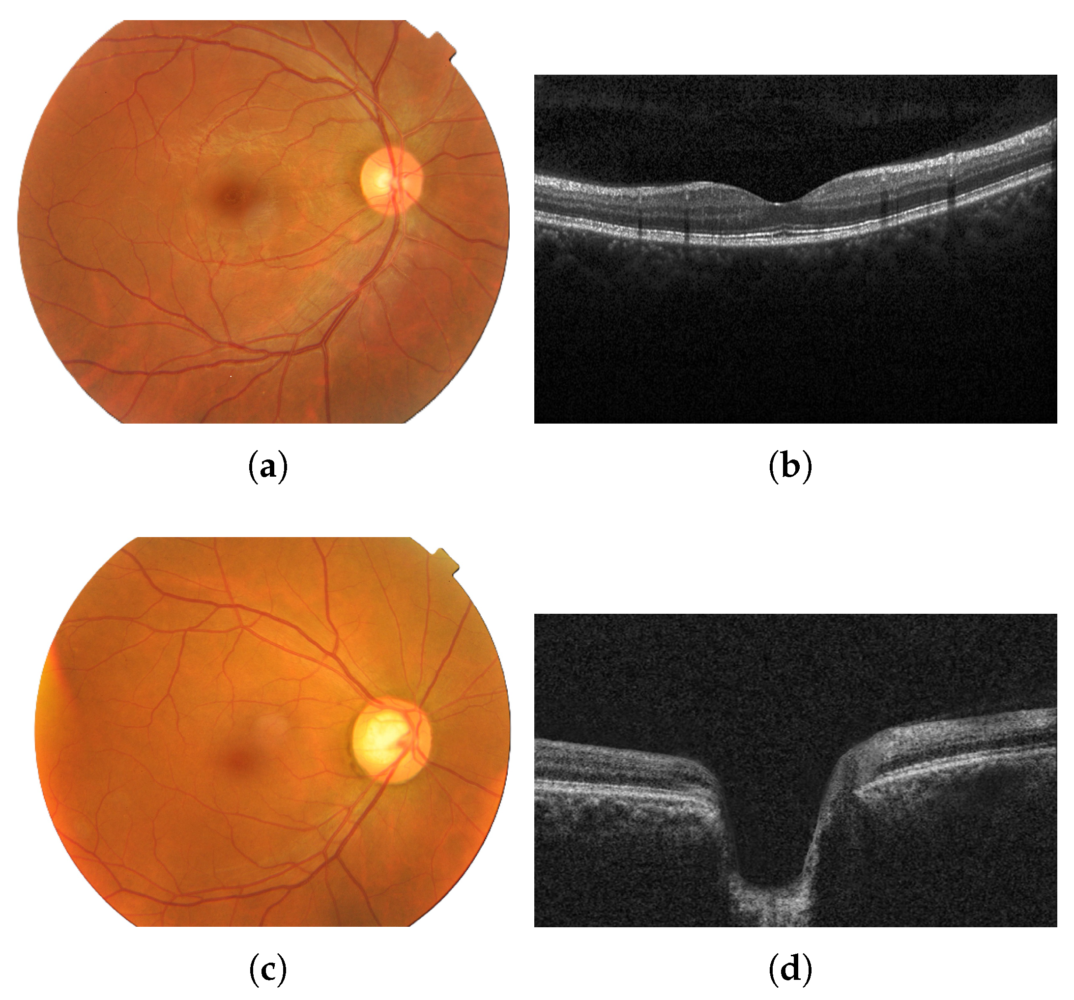
Figure 1.
Fundus image of an eye with no diseases (a) and the corresponding OCT image from the same healthy patient (b); fundus image of an eye with glaucoma (c) and the corresponding OCT image from the same glaucomatous patient (d). Images provided by Bangladesh Eye Hospital and Institute Ltd.
Figure 1.
Fundus image of an eye with no diseases (a) and the corresponding OCT image from the same healthy patient (b); fundus image of an eye with glaucoma (c) and the corresponding OCT image from the same glaucomatous patient (d). Images provided by Bangladesh Eye Hospital and Institute Ltd.
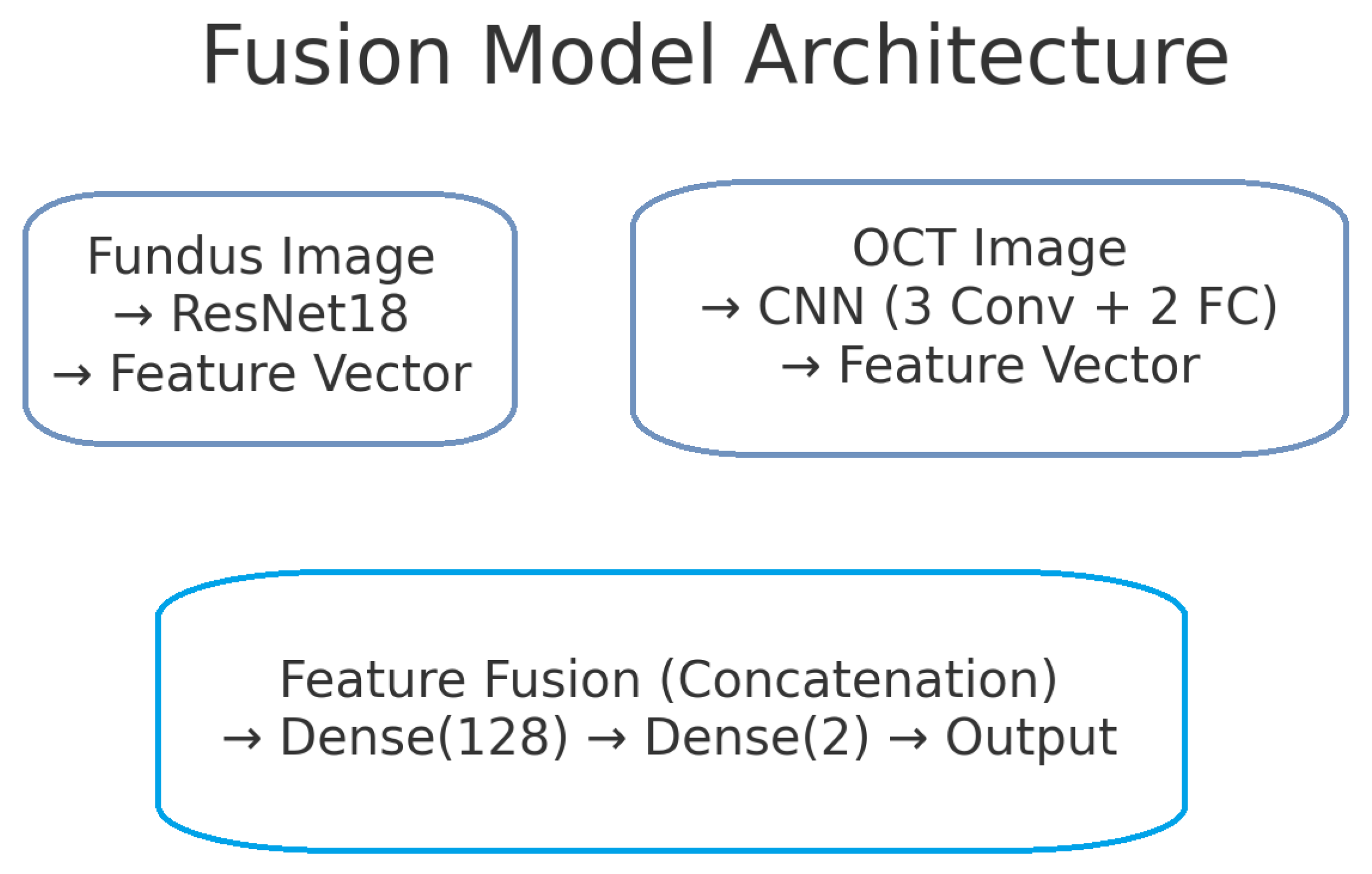
Figure 2.
Block diagram of the proposed dual-branch deep learning model for glaucoma detection. The left branch processes fundus images using a ResNet-18 network, producing a 128-dimensional fundus feature vector. The right branch processes OCT images with a custom CNN, producing a 128-dimensional OCT feature vector. These feature vectors are concatenated to form a 256-dimensional combined representation. A fully connected classifier (with a hidden layer and sigmoid output) takes the fused features and predicts the probability of glaucoma.
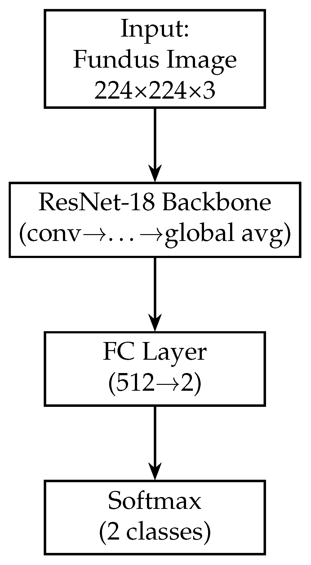
Figure 3.
Block diagram of the fundus-only model (ResNet-18). The fundus-only model takes a single 224 × 224 × 3 RGB fundus image as input, which is passed through the ResNet-18 backbone pre-trained on ImageNet. The backbone’s convolutional and residual layers extract hierarchical features of increasing abstraction, culminating in a 512-dimensional global average-pooled feature vector (GAP). This vector is fed into a fully connected layer that reduces from 512 to 2 units, and a final softmax activation produces class probabilities for “normal” versus “glaucoma”. All layers are trainable, enabling end-to-end fine-tuning on our fundus data.
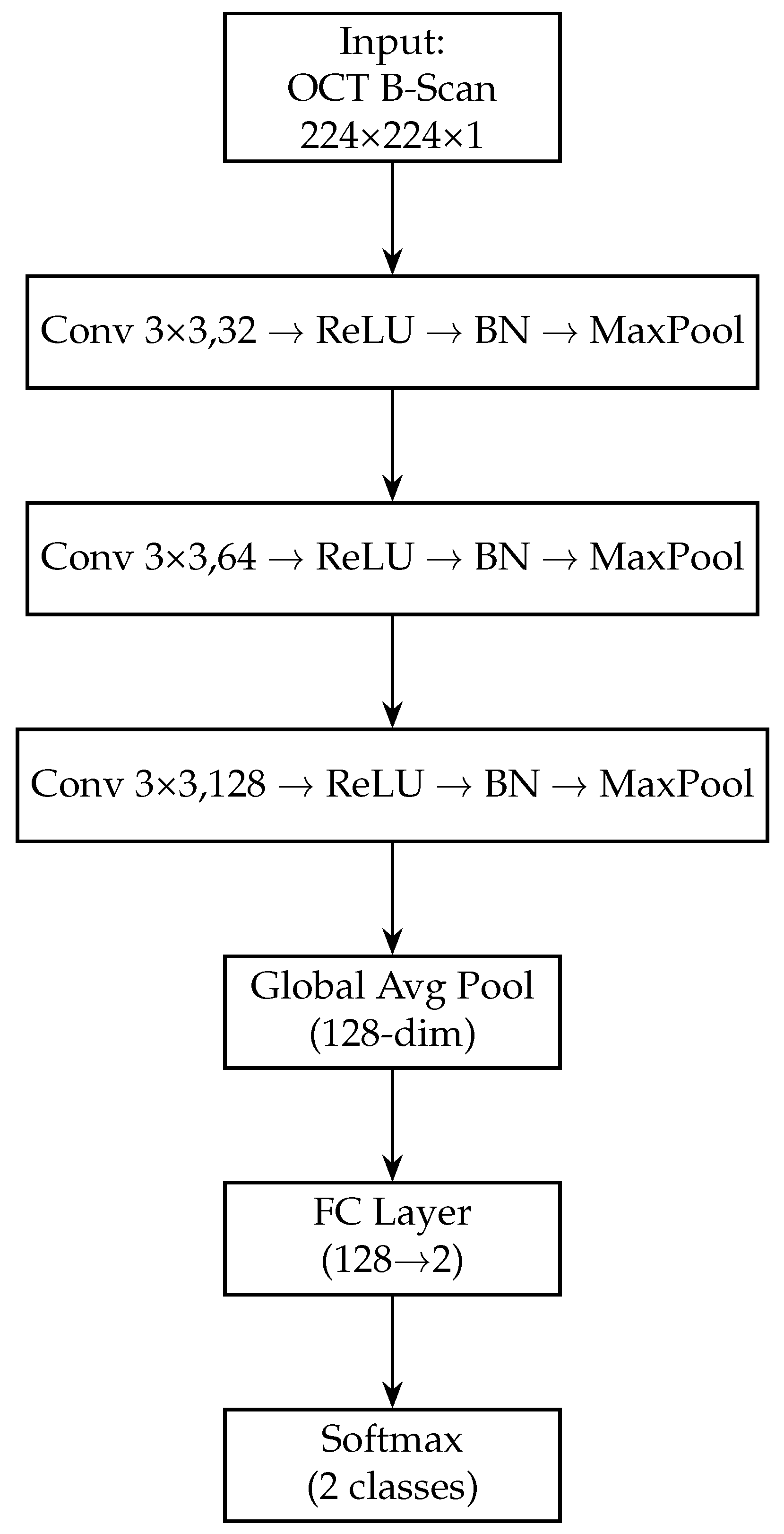
Figure 4.
Block diagram of the OCT-only model (custom CNN). The OCT-Only model accepts a single 224 × 224 × 1 grayscale B-scan. It employs three successive convolutional blocks—each consisting of a 3 × 3 conv layer, ReLU activation, batch normalisation and max-pooling—expanding channel depth from 32 → 64 → 128. A global average-pooling layer then collapses spatial dimensions to a 128-dimensional feature vector. A final fully connected layer maps these features to 2 logits, followed by a softmax to yield normal/glaucoma probabilities. This lightweight architecture captures cross-sectional RNFL and optic-nerve-head structures.
Figure 5.
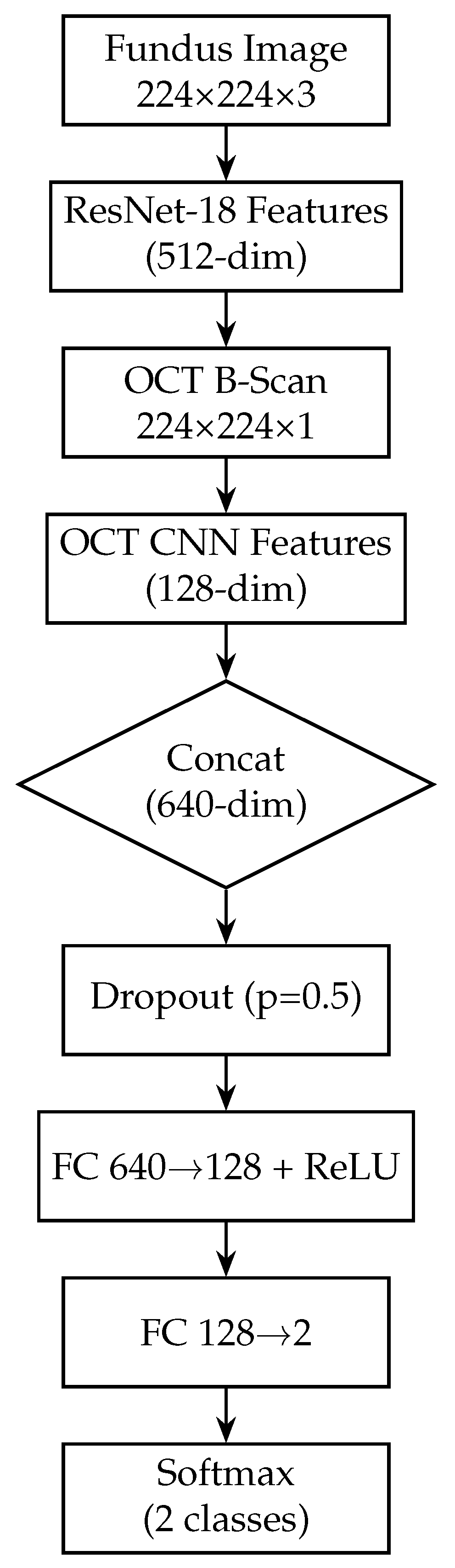
Block diagram of the fusion model, combining fundus and OCT features. The fusion model integrates both modalities by first extracting a 512-dim feature vector from the fundus branch and a 128-dim vector from the OCT branch. These vectors are concatenated into a 640-dim joint representation, to which dropout (p = 0.5) is applied for regularisation. Two fully connected layers with ReLU activations (640 → 128 → 2) then learn to combine cross-modal information. A softmax yields the final glaucoma probability. By fusing mid-level features, this design leverages complementary surface and depth cues for improved diagnostic accuracy.
Figure 5.
Block diagram of the fusion model, combining fundus and OCT features. The fusion model integrates both modalities by first extracting a 512-dim feature vector from the fundus branch and a 128-dim vector from the OCT branch. These vectors are concatenated into a 640-dim joint representation, to which dropout (p = 0.5) is applied for regularisation. Two fully connected layers with ReLU activations (640 → 128 → 2) then learn to combine cross-modal information. A softmax yields the final glaucoma probability. By fusing mid-level features, this design leverages complementary surface and depth cues for improved diagnostic accuracy.
Figure 6.
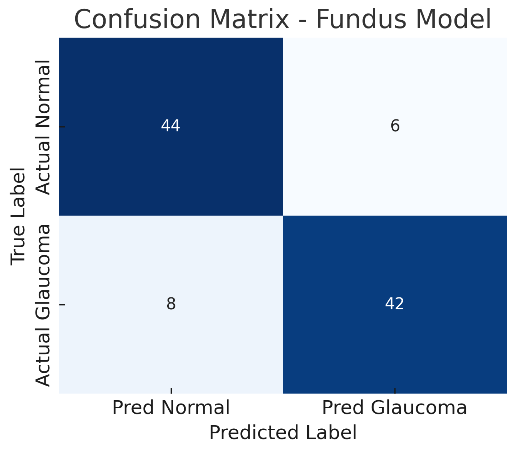
Confusion matrix for fundus-only model. True negatives (TN), false positives (FP), false negatives (FN), and true positives (TP) are shown.
Figure 6.
Confusion matrix for fundus-only model. True negatives (TN), false positives (FP), false negatives (FN), and true positives (TP) are shown.
Figure 7.
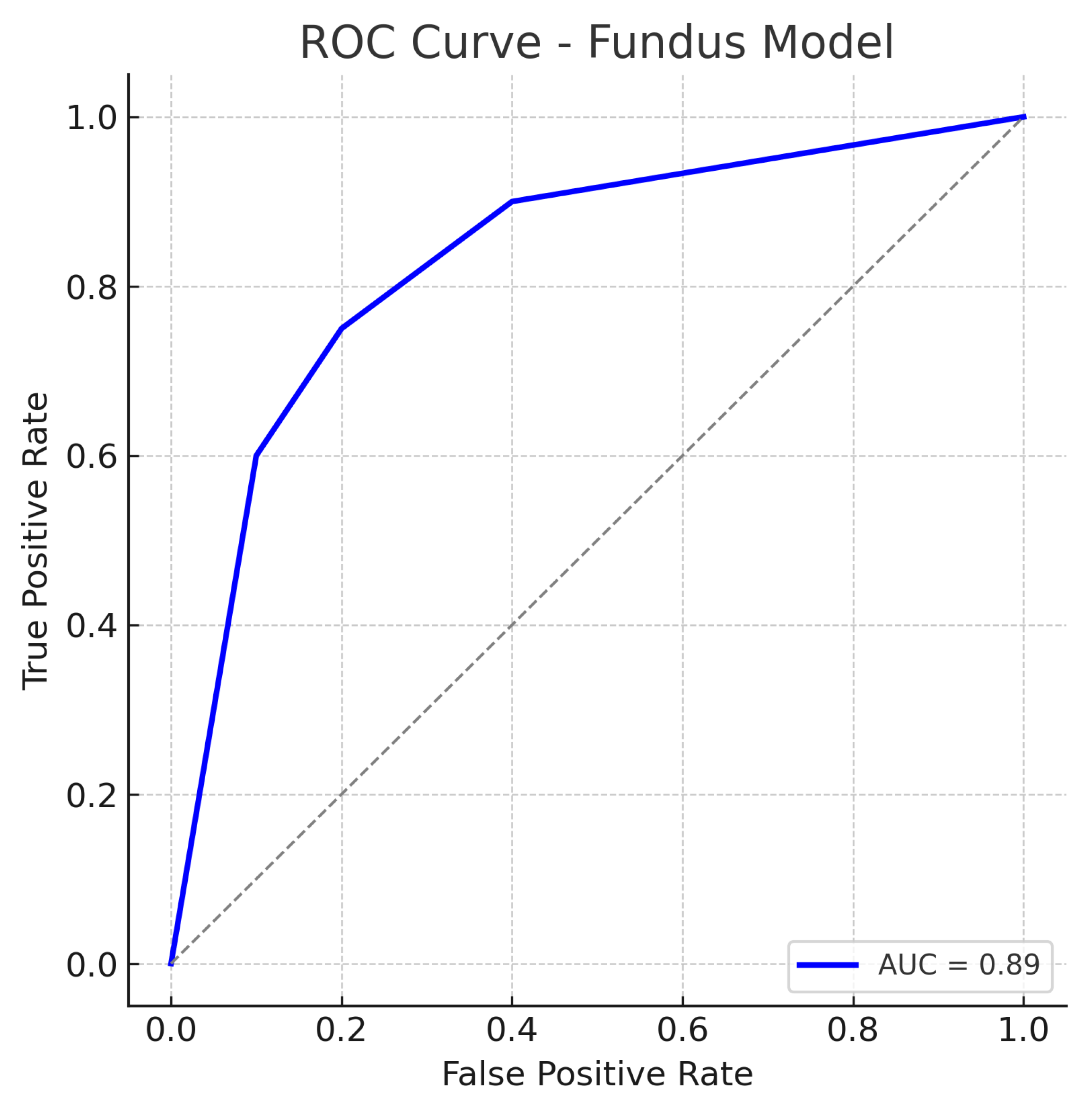
ROC curve for the fundus-only (ResNet18) model. The true positive rate (sensitivity) is plotted against the false positive rate (1−specificity). The fundus model achieves an AUC of approximately 0.89, indicating robust performance in distinguishing glaucomatous from healthy eyes. The curve bows toward the top-left corner, reflecting a good trade-off between sensitivity and specificity. The dotted diagonal line represents chance performance.
Figure 7.
ROC curve for the fundus-only (ResNet18) model. The true positive rate (sensitivity) is plotted against the false positive rate (1−specificity). The fundus model achieves an AUC of approximately 0.89, indicating robust performance in distinguishing glaucomatous from healthy eyes. The curve bows toward the top-left corner, reflecting a good trade-off between sensitivity and specificity. The dotted diagonal line represents chance performance.
Figure 8.
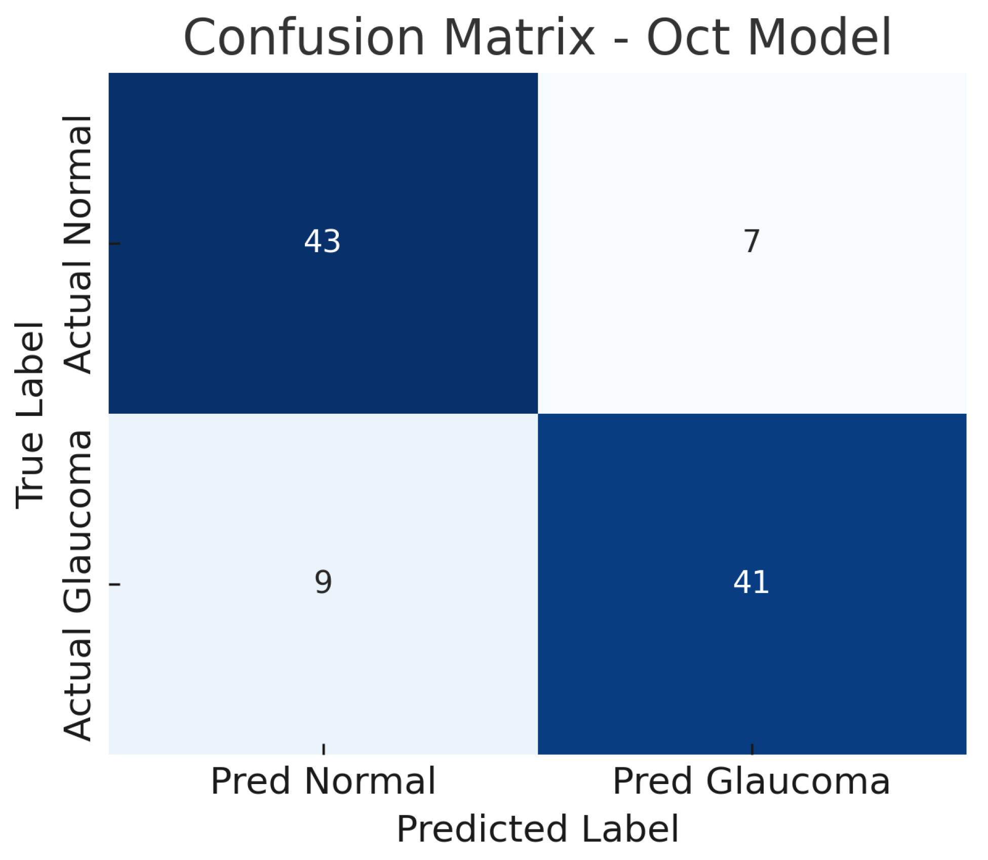
Confusion matrix for OCT-only model. True negatives (TN), false positives (FP), false negatives (FN), and true positives (TP) are shown.
Figure 8.
Confusion matrix for OCT-only model. True negatives (TN), false positives (FP), false negatives (FN), and true positives (TP) are shown.
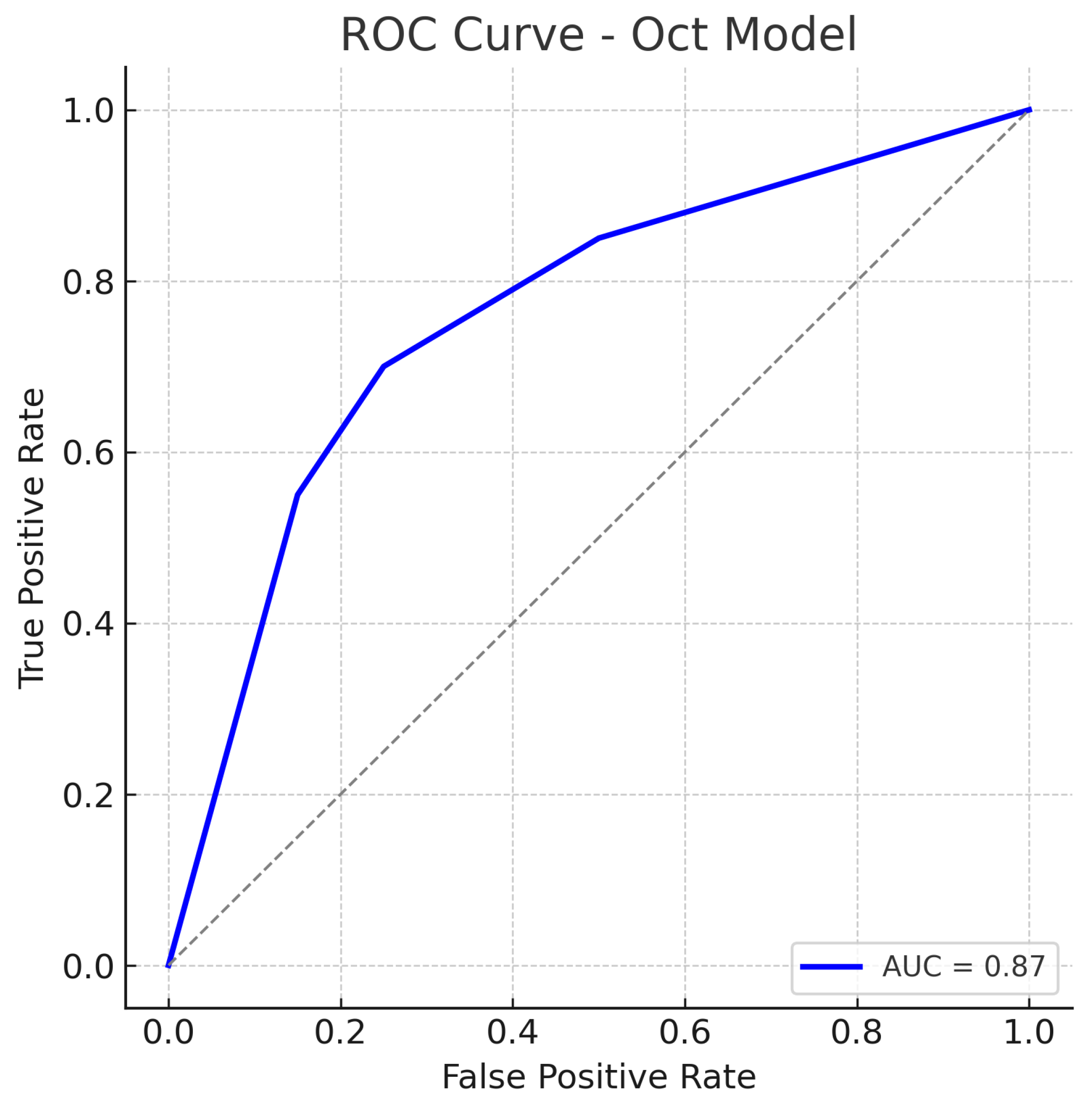
Figure 9.
ROC curve for the OCT-Only (Custom CNN) model. The model attains an AUC of approximately 0.87. The curve is slightly below that of the fundus model, reflecting marginally lower overall performance. Nonetheless, the OCT model’s ROC curve still shows a substantial improvement over chance, indicating that the OCT-based features carry significant information for glaucoma detection. The dotted diagonal line represents chance performance.
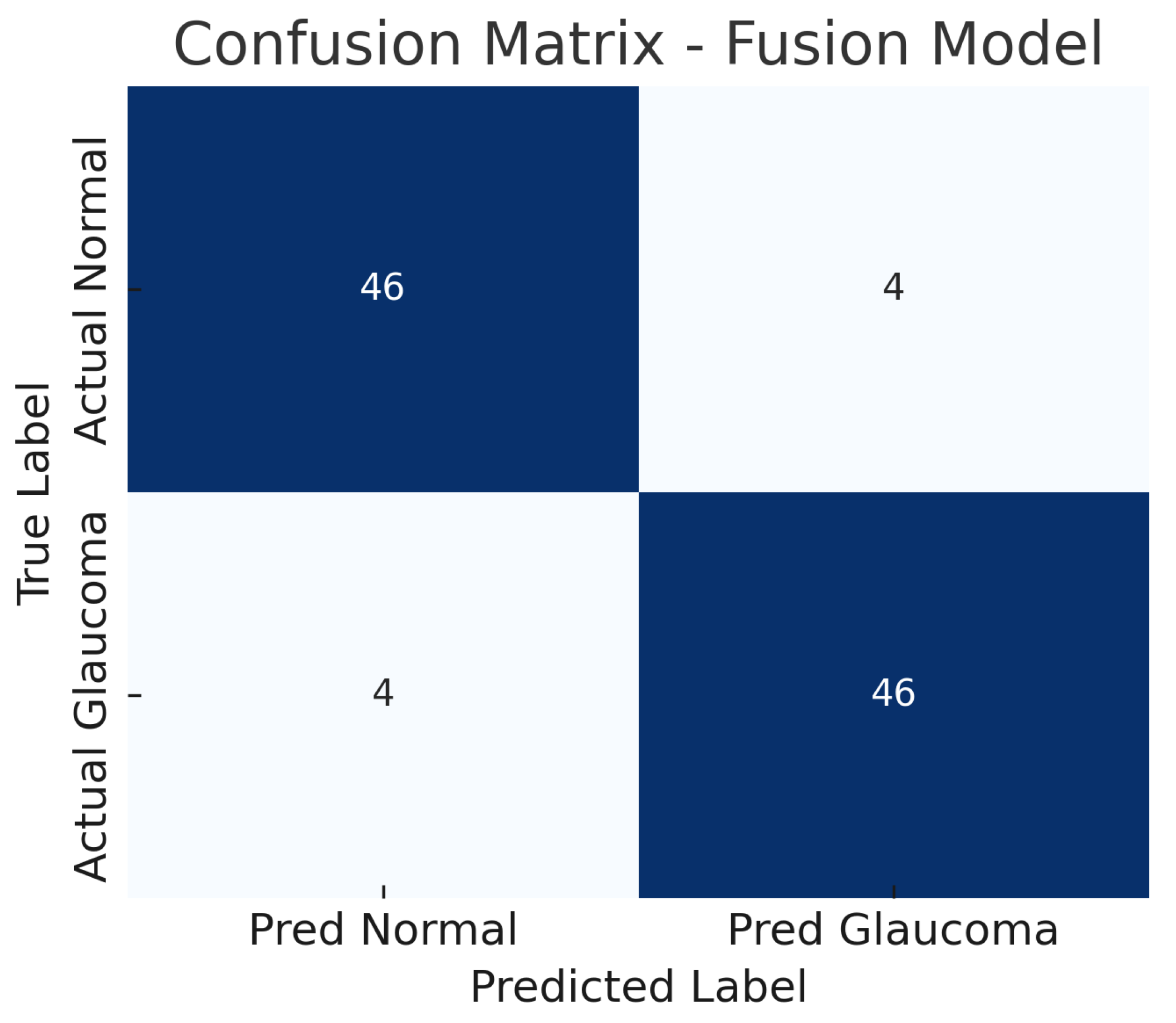
Figure 10.
Confusion matrix for fusion model. True negatives (TN), false positives (FP), false negatives (FN), and true positives (TP) are shown.
Figure 10.
Confusion matrix for fusion model. True negatives (TN), false positives (FP), false negatives (FN), and true positives (TP) are shown.
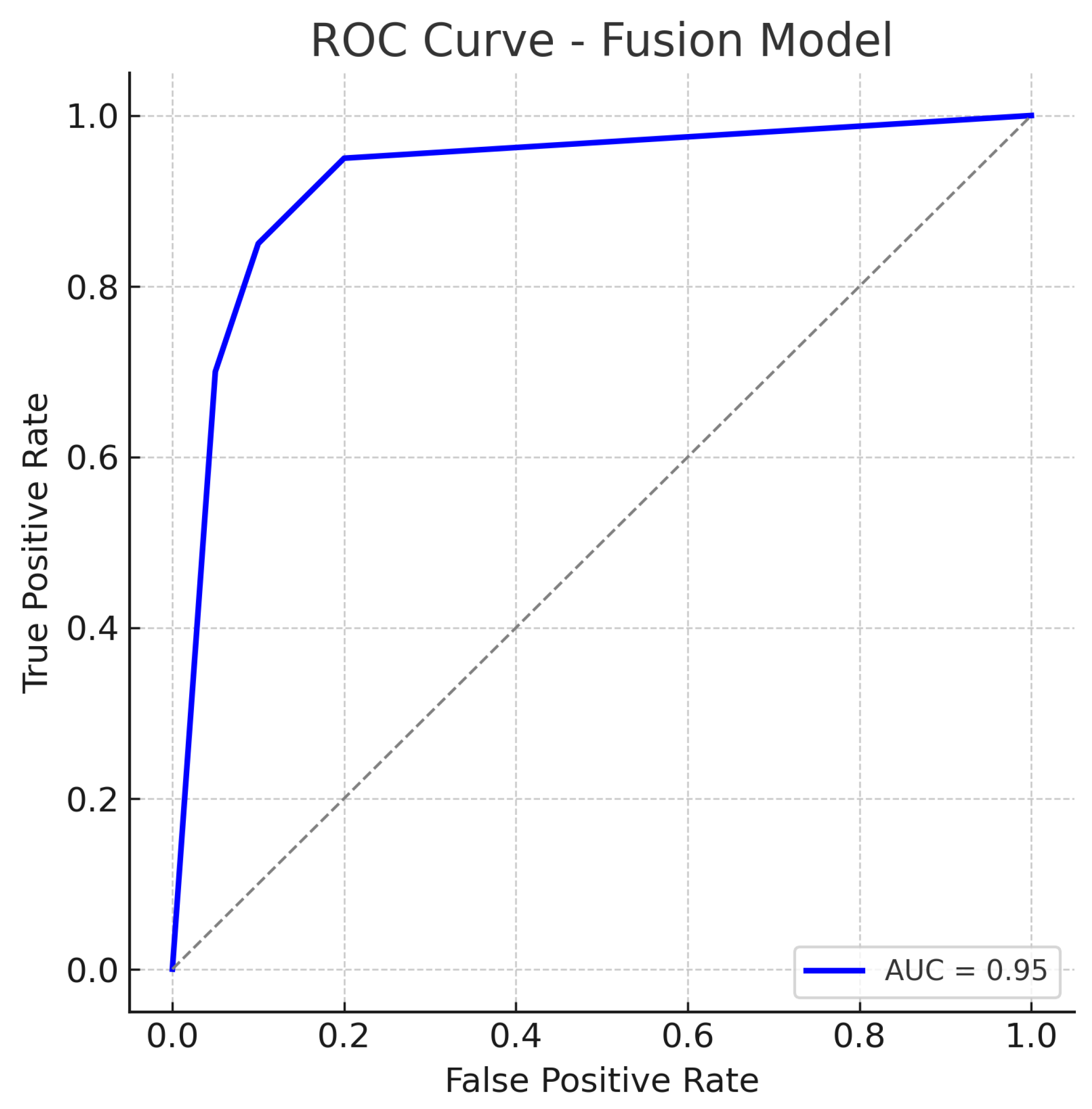
Figure 11.
ROC curve for the Fusion (Fundus + OCT) model. The fusion model achieves an AUC of approximately 0.95, markedly higher than the single-modality models. The dotted diagonal line represents chance performance.
Figure 11.
ROC curve for the Fusion (Fundus + OCT) model. The fusion model achieves an AUC of approximately 0.95, markedly higher than the single-modality models. The dotted diagonal line represents chance performance.
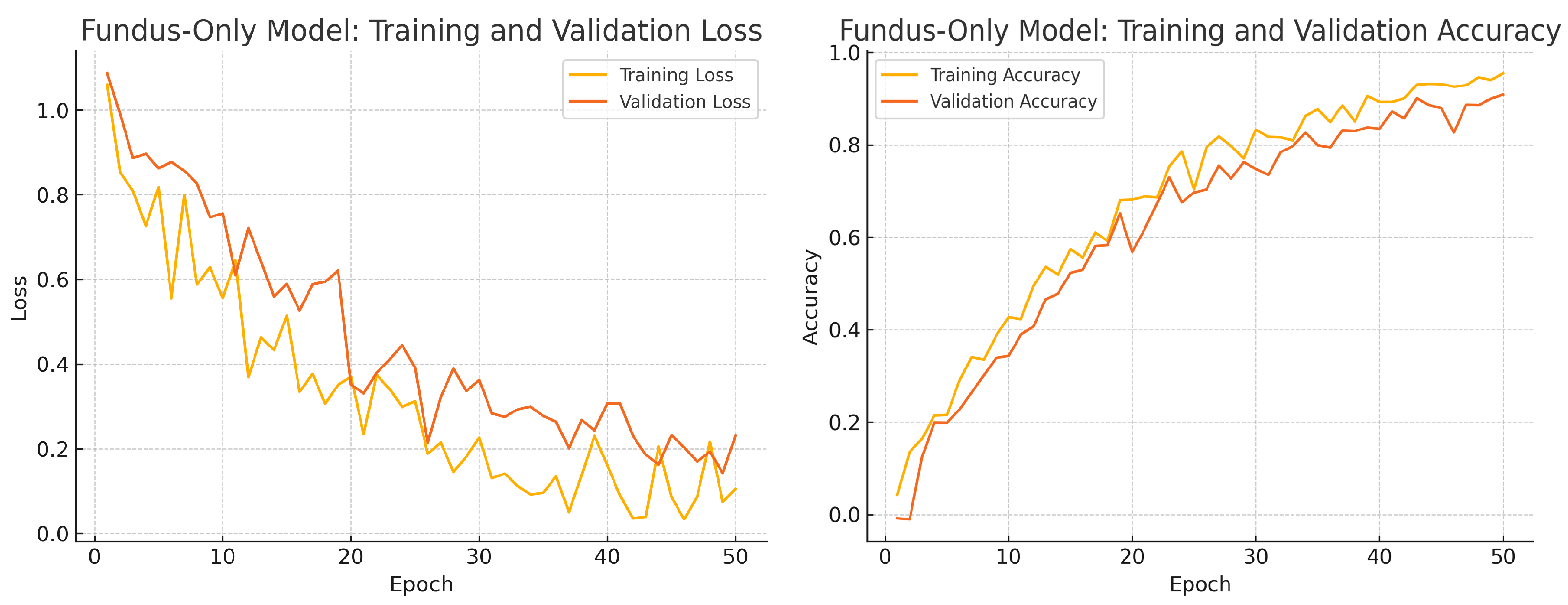
Figure 12.
Fundus-only model training progress over 50 epochs. Left: Training (yellow) and validation (orange) loss. Right: Training (yellow) and validation (orange) accuracy.
Figure 12.
Fundus-only model training progress over 50 epochs. Left: Training (yellow) and validation (orange) loss. Right: Training (yellow) and validation (orange) accuracy.
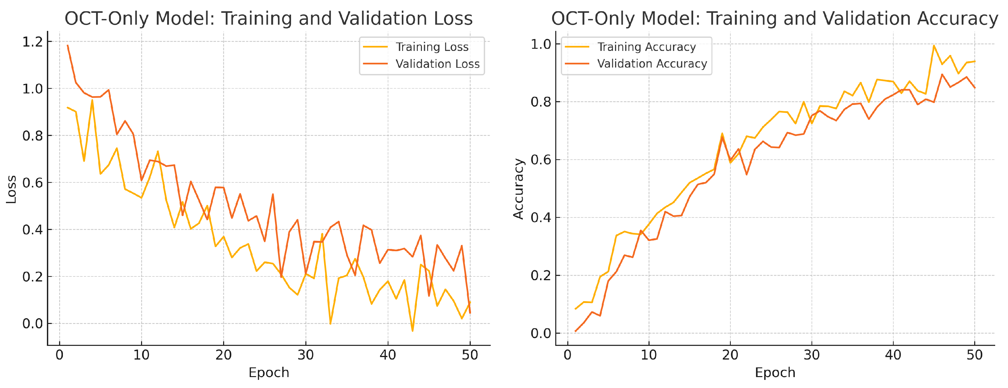
Figure 13.
OCT-only model training progress over 50 epochs. Left: Training (yellow) and validation (orange) loss. Right: Training (yellow) and validation (orange) accuracy.
Figure 13.
OCT-only model training progress over 50 epochs. Left: Training (yellow) and validation (orange) loss. Right: Training (yellow) and validation (orange) accuracy.
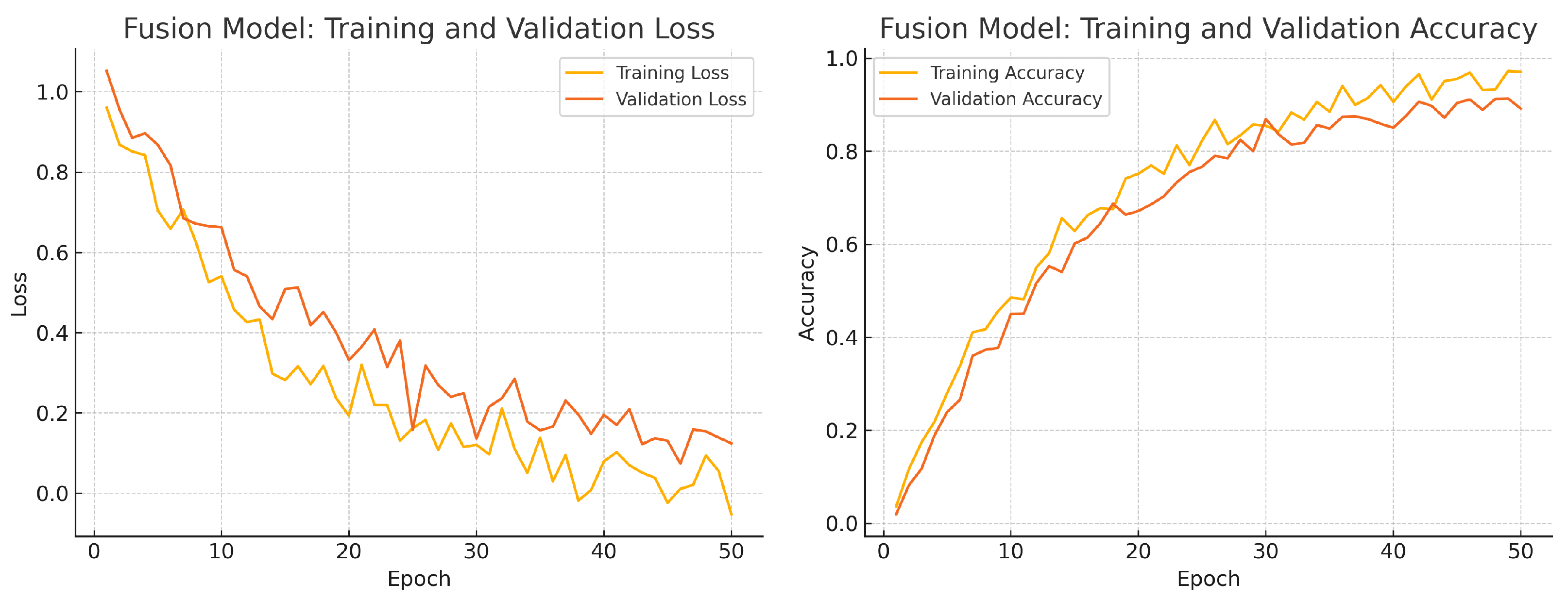
Figure 14.
Fusion model training progress over 50 epochs. Left: Training (yellow) and validation (orange) loss. Right: Training (yellow) and validation (orange) accuracy.
Figure 14.
Fusion model training progress over 50 epochs. Left: Training (yellow) and validation (orange) loss. Right: Training (yellow) and validation (orange) accuracy.
Figure 15.
Aggregated confusion matrix for the fusion-only model (five-fold CV). True negatives (TN), false positives (FP), false negatives (FN), and true positives (TP) are shown.
Figure 15.
Aggregated confusion matrix for the fusion-only model (five-fold CV). True negatives (TN), false positives (FP), false negatives (FN), and true positives (TP) are shown.
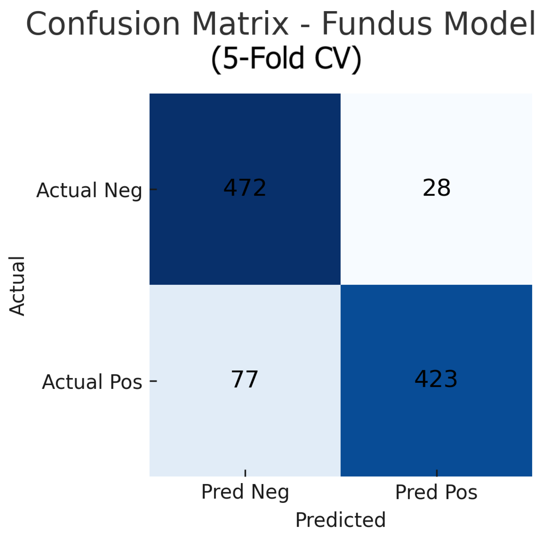
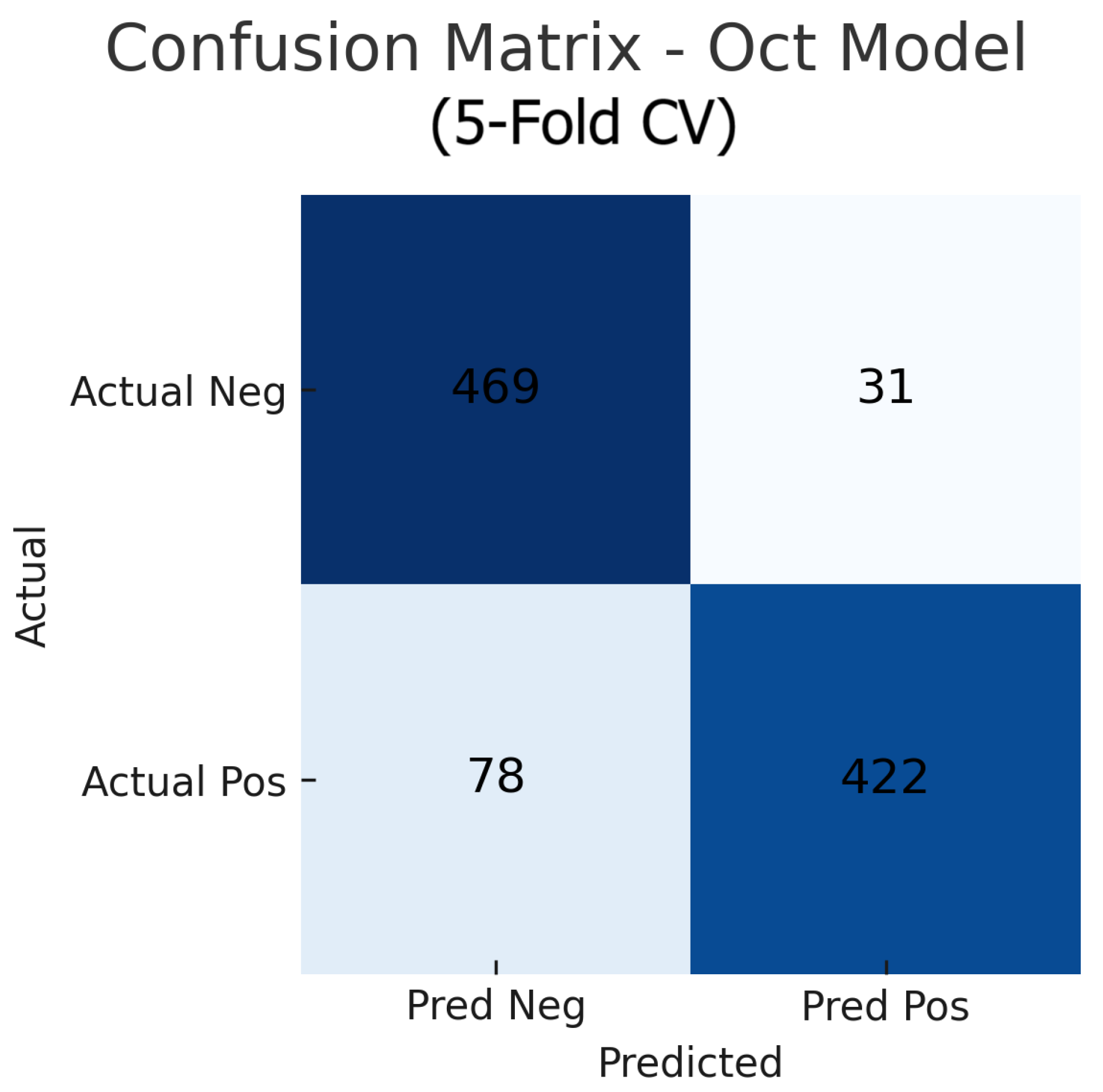
Figure 16.
Aggregated confusion matrix for the OCT-only model (five-fold CV). True negatives (TN), false positives (FP), false negatives (FN), and true positives (TP) are shown.
Figure 16.
Aggregated confusion matrix for the OCT-only model (five-fold CV). True negatives (TN), false positives (FP), false negatives (FN), and true positives (TP) are shown.
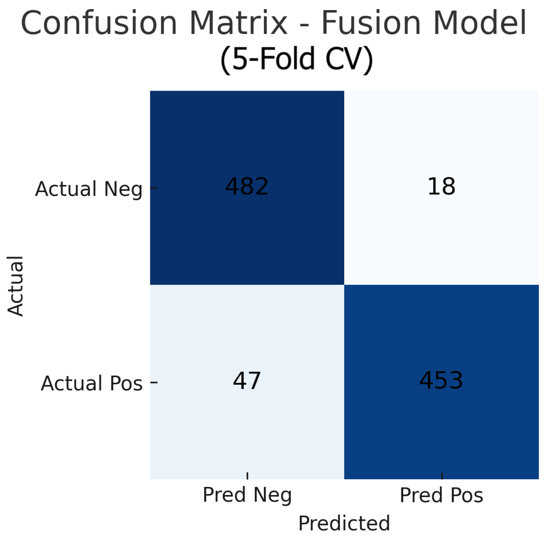
Figure 17.
Aggregated confusion matrix for the fusion (fundus+OCT) model (five-fold CV). True negatives (TN), false positives (FP), false negatives (FN), and true positives (TP) are shown.
Figure 17.
Aggregated confusion matrix for the fusion (fundus+OCT) model (five-fold CV). True negatives (TN), false positives (FP), false negatives (FN), and true positives (TP) are shown.
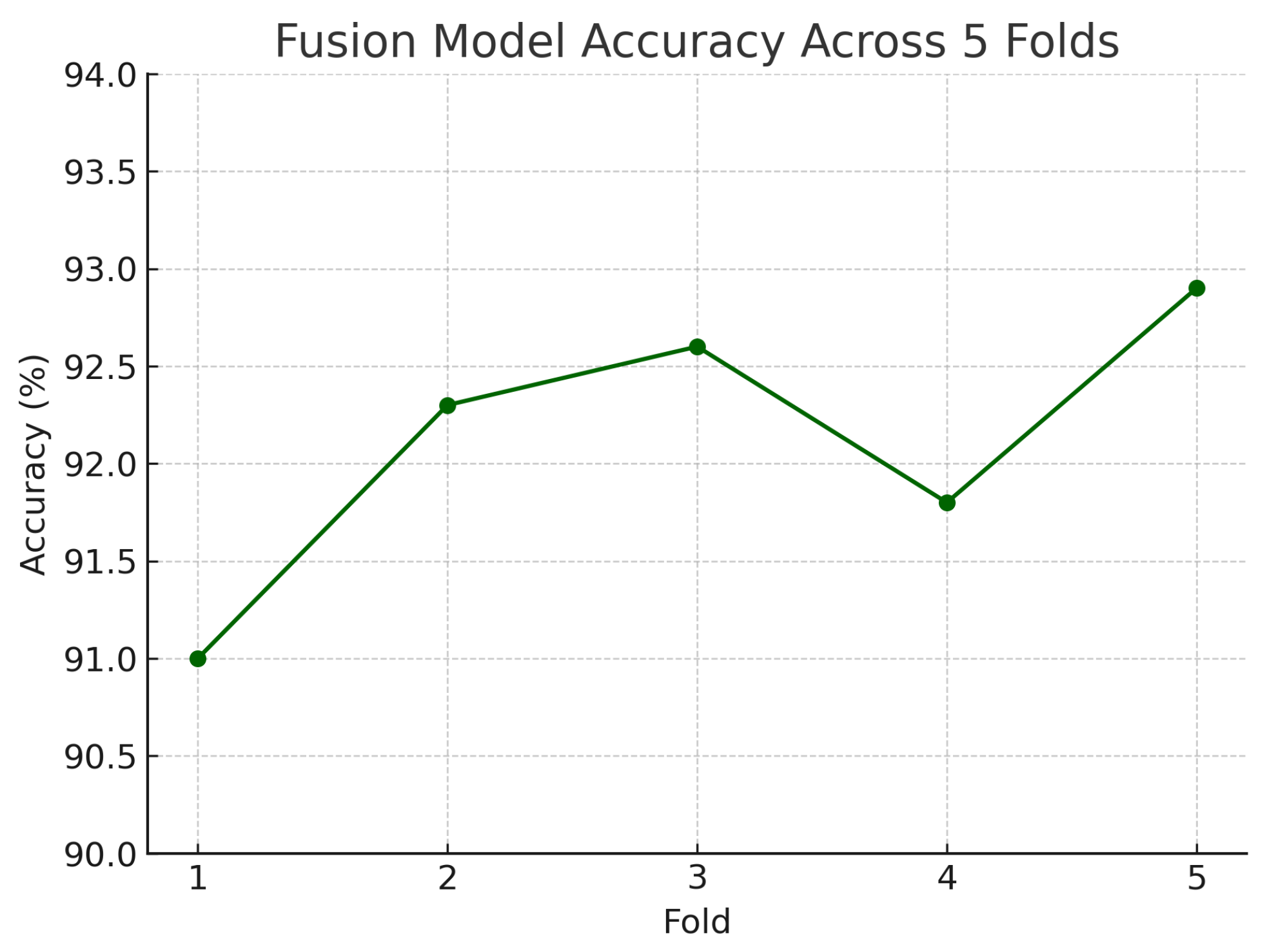
Figure 18.
Accuracy of the fusion model across each fold in five-fold cross-validation. Performance remained consistent, ranging from 91.0% to 92.9%.
Figure 18.
Accuracy of the fusion model across each fold in five-fold cross-validation. Performance remained consistent, ranging from 91.0% to 92.9%.
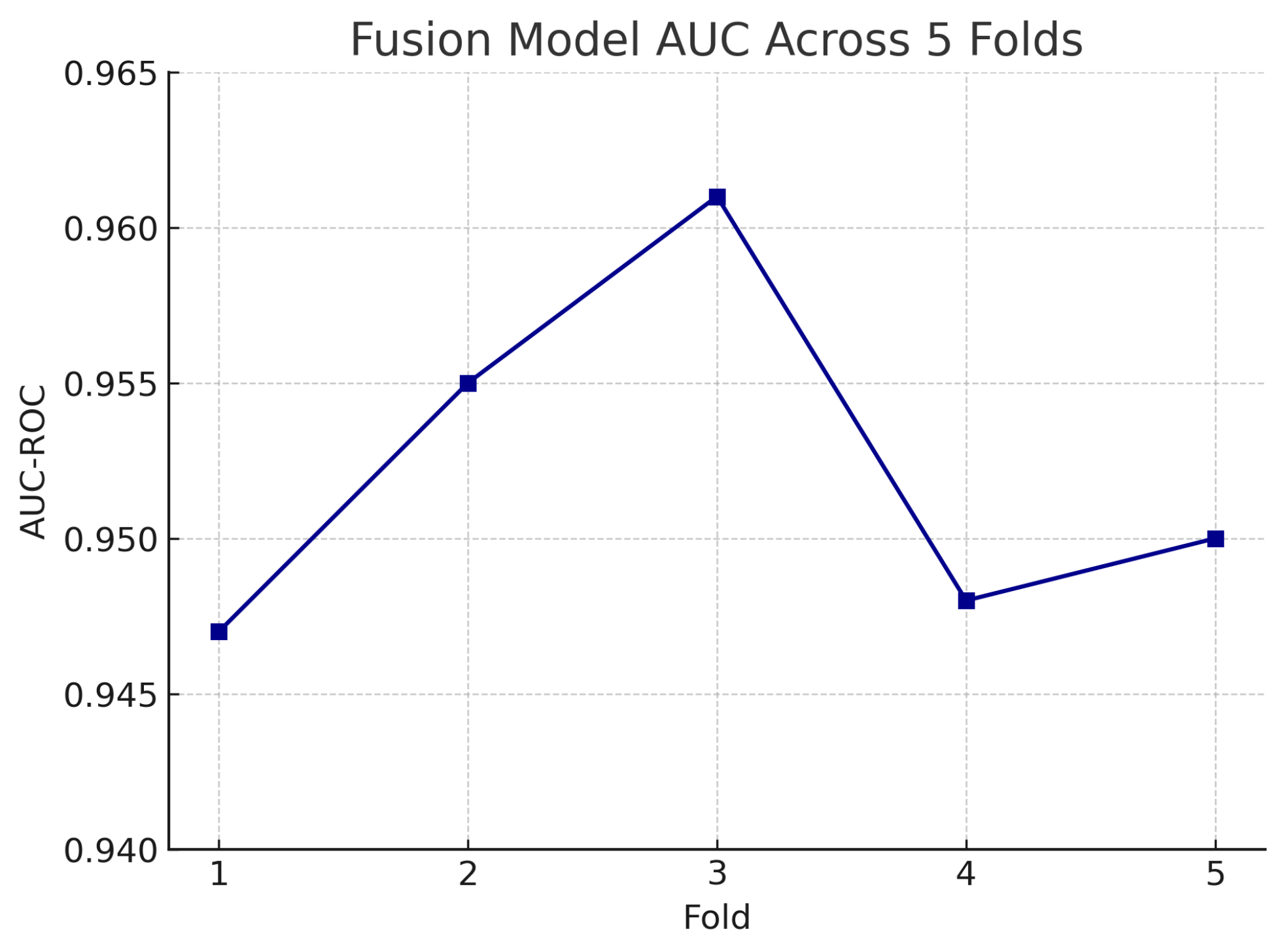
Figure 19.
AUC-ROC of the fusion model across each fold in five-fold cross-validation. AUC values remain high and stable, demonstrating model robustness.
Figure 19.
AUC-ROC of the fusion model across each fold in five-fold cross-validation. AUC values remain high and stable, demonstrating model robustness.
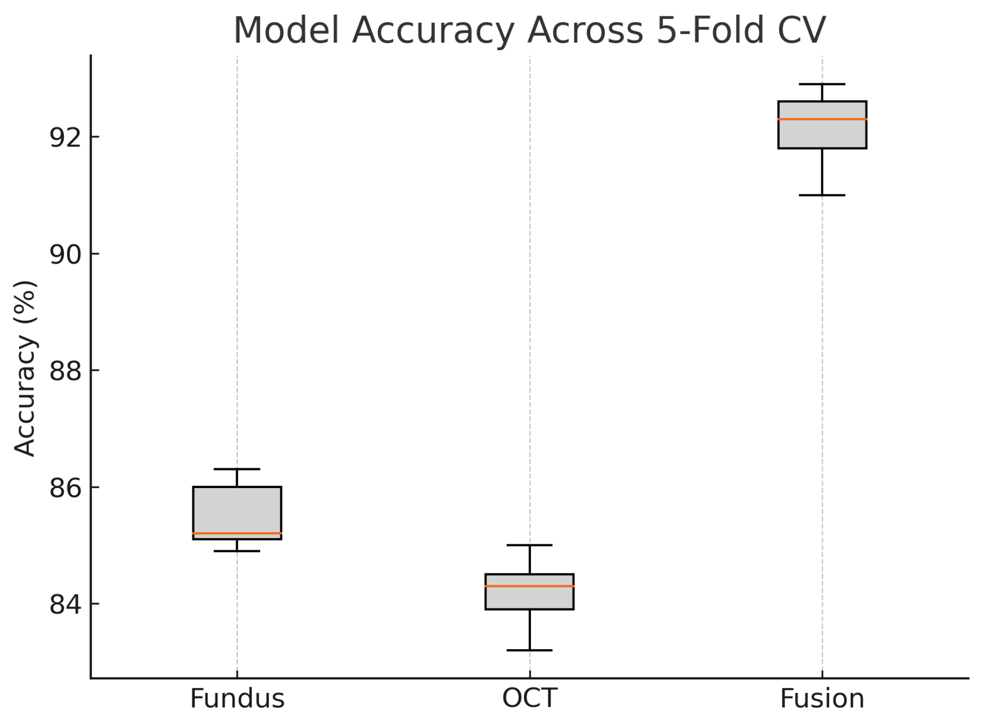
Figure 20.
Boxplot of classification accuracy across five-fold cross-validation for fundus-only, OCT-only, and fusion models. The fusion model demonstrates superior and more stable performance.
Figure 20.
Boxplot of classification accuracy across five-fold cross-validation for fundus-only, OCT-only, and fusion models. The fusion model demonstrates superior and more stable performance.
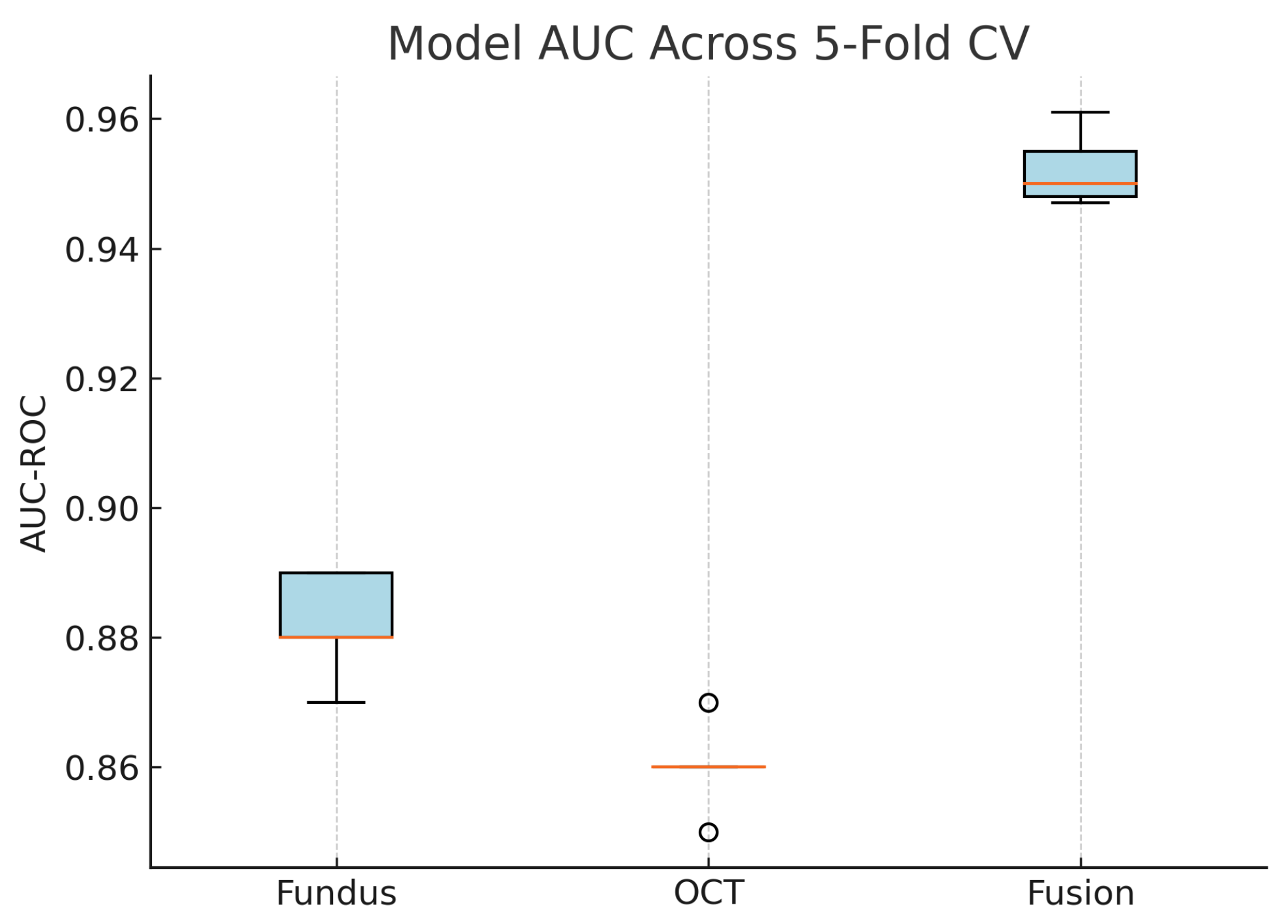
Figure 21.
Boxplot of AUC-ROC across five-fold cross-validation for each model. The fusion model shows both the highest and most consistent AUC values.
Figure 21.
Boxplot of AUC-ROC across five-fold cross-validation for each model. The fusion model shows both the highest and most consistent AUC values.
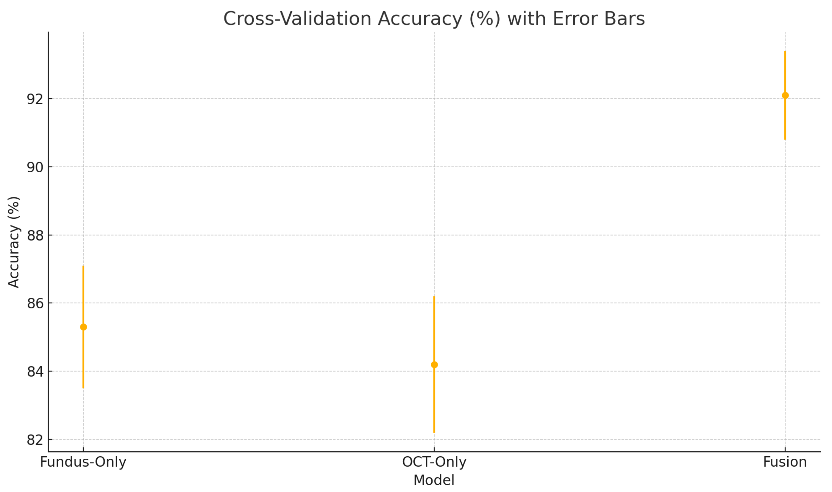
Figure 22.
Cross-validation accuracy (%) variability across five folds for the fundus-only, OCT-only, and fusion models. Error bars represent ± one standard deviation from the mean accuracy.
Figure 22.
Cross-validation accuracy (%) variability across five folds for the fundus-only, OCT-only, and fusion models. Error bars represent ± one standard deviation from the mean accuracy.
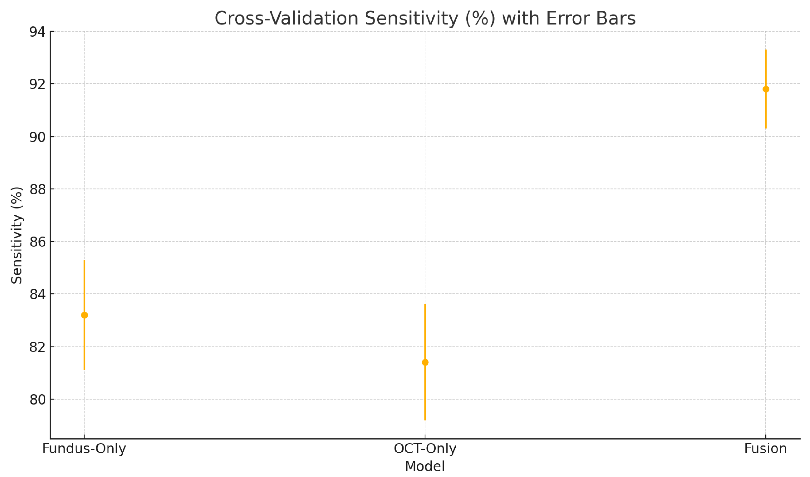
Figure 23.
Cross-validation sensitivity (%) variability across five folds for the fundus-only, OCT-only, and fusion models. Error bars represent ± one standard deviation from the mean sensitivity.
Figure 23.
Cross-validation sensitivity (%) variability across five folds for the fundus-only, OCT-only, and fusion models. Error bars represent ± one standard deviation from the mean sensitivity.
Figure 24.
Cross-validation specificity (%) variability across five folds for the fundus-only, OCT-only, and fusion models. Error bars represent ± one standard deviation from the mean specificity.
Figure 24.
Cross-validation specificity (%) variability across five folds for the fundus-only, OCT-only, and fusion models. Error bars represent ± one standard deviation from the mean specificity.
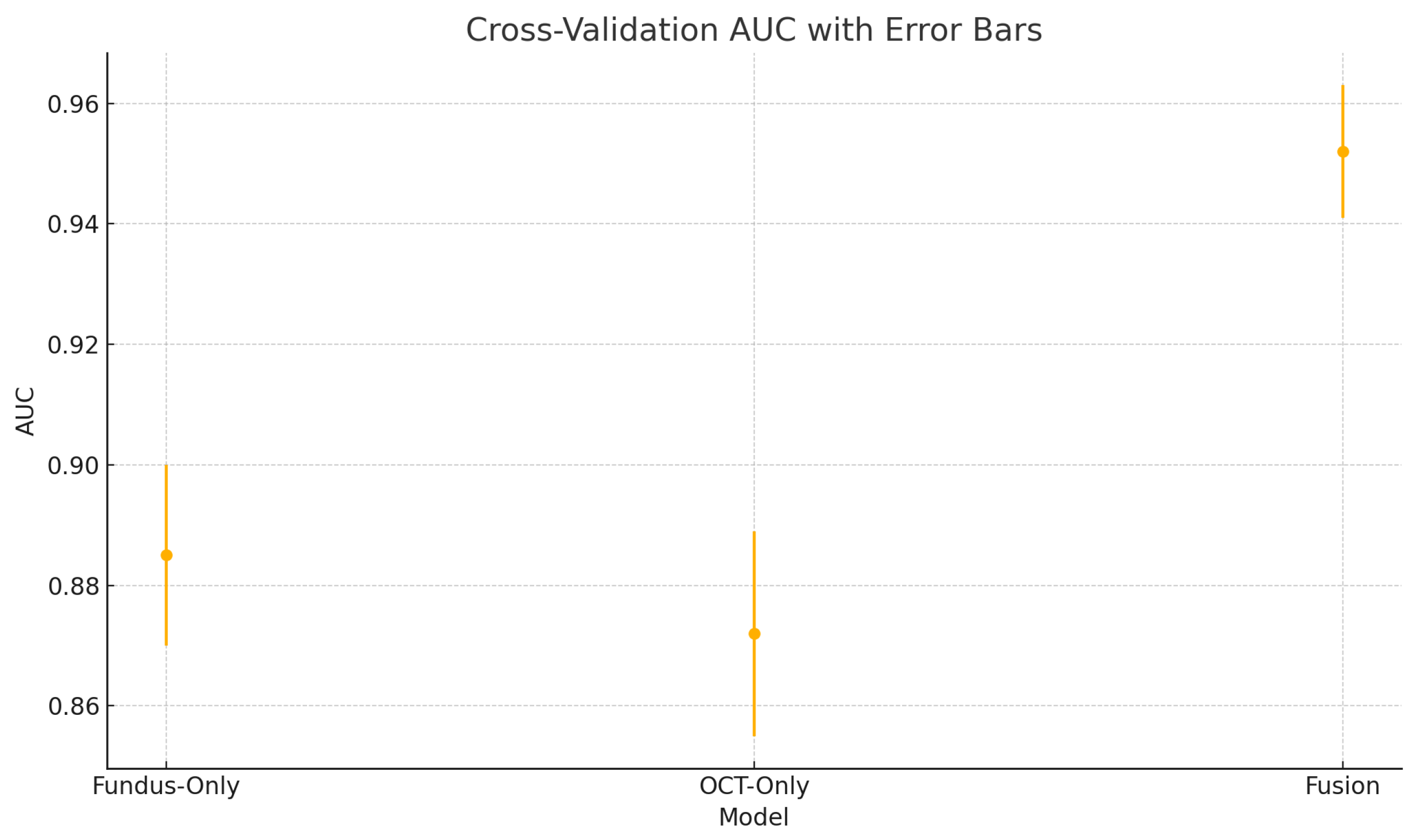
Figure 25.
Cross-validation area under the ROC curve (AUC) variability across five folds for the fundus-only, OCT-only, and fusion models. Error bars represent ± one standard deviation from the mean AUC.
Figure 25.
Cross-validation area under the ROC curve (AUC) variability across five folds for the fundus-only, OCT-only, and fusion models. Error bars represent ± one standard deviation from the mean AUC.
Table 2.
Summary of the glaucoma dataset from Bangladesh Eye Hospital. Each eye contributes one fundus and one OCT image.
Table 2.
Summary of the glaucoma dataset from Bangladesh Eye Hospital. Each eye contributes one fundus and one OCT image.
| Category | Eyes | Fundus Images | OCT Images | Total Images |
|---|
| Normal | 108 | 108 | 108 | 216 |
| Glaucoma | 100 | 100 | 100 | 200 |
| Total | 208 | 208 | 208 | 416 |
Table 3.
Architecture of the custom OCT CNN branch. Conv = convolutional layer, BN = batch normalisation, MP = max-pooling, GAP = global average pooling, FC = fully connected layer. The output size is listed as (H × W × C) for feature maps and as a vector length for fully connected outputs.
Table 3.
Architecture of the custom OCT CNN branch. Conv = convolutional layer, BN = batch normalisation, MP = max-pooling, GAP = global average pooling, FC = fully connected layer. The output size is listed as (H × W × C) for feature maps and as a vector length for fully connected outputs.
| Layer | Filter Size | Output Channels | Output Size | Activation |
|---|
| Input OCT image | – | 1 | 224 × 224 × 1 | – |
| Conv1 + BN + ReLU | 3 × 3/1 | 32 | 224 × 224 × 32 | ReLU |
| Max Pool1 | 2 × 2/2 | – | 112 × 112 × 32 | – |
| Conv2 + BN + ReLU | 3 × 3/1 | 64 | 112 × 112 × 64 | ReLU |
| Max Pool2 | 2 × 2/2 | – | 56 × 56 × 64 | – |
| Conv3 + BN + ReLU | 3 × 3/1 | 128 | 56 × 56 × 128 | ReLU |
| Max Pool3 | 2 × 2/2 | – | 28 × 28 × 128 | – |
| Conv4 + BN + ReLU | 3 × 3/1 | 256 | 28 × 28 × 256 | ReLU |
| Global Avg Pool | – | – | 1 × 1 × 256 | – |
| Flatten | – | – | 256 (vector) | – |
| FC (OCT feature) | – | 128 | 128 (vector) | ReLU |
Table 4.
Comparison of evaluation metrics across models. Acc = Accuracy, Sen = Sensitivity, Spec = Specificity.
Table 4.
Comparison of evaluation metrics across models. Acc = Accuracy, Sen = Sensitivity, Spec = Specificity.
| Model | Acc | Sens | Spec | AUC-ROC |
|---|
| Fundus-Only (ResNet18) | 86% | 84% | 88% | 0.89 |
| OCT-Only (Custom CNN) | 84% | 82% | 86% | 0.87 |
| Fusion (Fundus + OCT) | 92% | 92% | 92% | 0.95 |
Table 5.
Five-fold cross-validation results (average ± standard deviation).
Table 5.
Five-fold cross-validation results (average ± standard deviation).
| Model | Accuracy (%) | Sensitivity (%) | Specificity (%) | AUC |
|---|
| Fundus-Only | 85.3 ± 1.8 | 83.2 ± 2.1 | 87.1 ± 1.6 | 0.885 ± 0.015 |
| OCT-Only | 84.2 ± 2.0 | 81.4 ± 2.2 | 86.5 ± 1.8 | 0.872 ± 0.017 |
| Fusion | 92.1 ± 1.3 | 91.8 ± 1.5 | 92.4 ± 1.2 | 0.952 ± 0.011 |
Table 6.
Performance comparison with previous studies.
Table 6.
Performance comparison with previous studies.
| Ref | Input | Model | Dataset | Acc% | Spec% | Sens% | AUC |
|---|
| [14] | Fundus | VGG19 | RIM-ONE | | 89 | 87 | 0.94 |
| [39] | OCT | ResNet18 | Private | 91 | 91.3 | 89.1 | 0.96 |
| [46] | Fundus | ResNet50 | RIM-ONE | 95.49 | 88.88 | 97.59 | |
| [75] | OCT | ResNet18 | Private | | | | 0.937 |
| [74] | Fundus | CNN | Private | | | | 0.945 |
| [76] | OCT | DruNet | Private | | 99 | 90 | 0.96 |
| Ours | Fundus | ResNet18 | Private | 85.3 | 87.1 | 83.2 | 0.885 |
| Ours | OCT | CNN | Private | 84.2 | 86.5 | 81.4 | 0.872 |
| Ours | Fundus+OCT | CNN | Private | 92.1 | 92.4 | 91.8 | 0.952 |


 ,
, 