
Bearing Fault Diagnosis via Stepwise Sparse Regularization with an Adaptive Sparse Dictionary


Abstract
1. Introduction
2. Theoretical Framework
2.1. Sparse Regularization
2.2. Construction of the Sparse Dictionary
3. Stepwise Sparse Regularization with an Adaptive Sparse Dictionary
3.1. Model Establishment
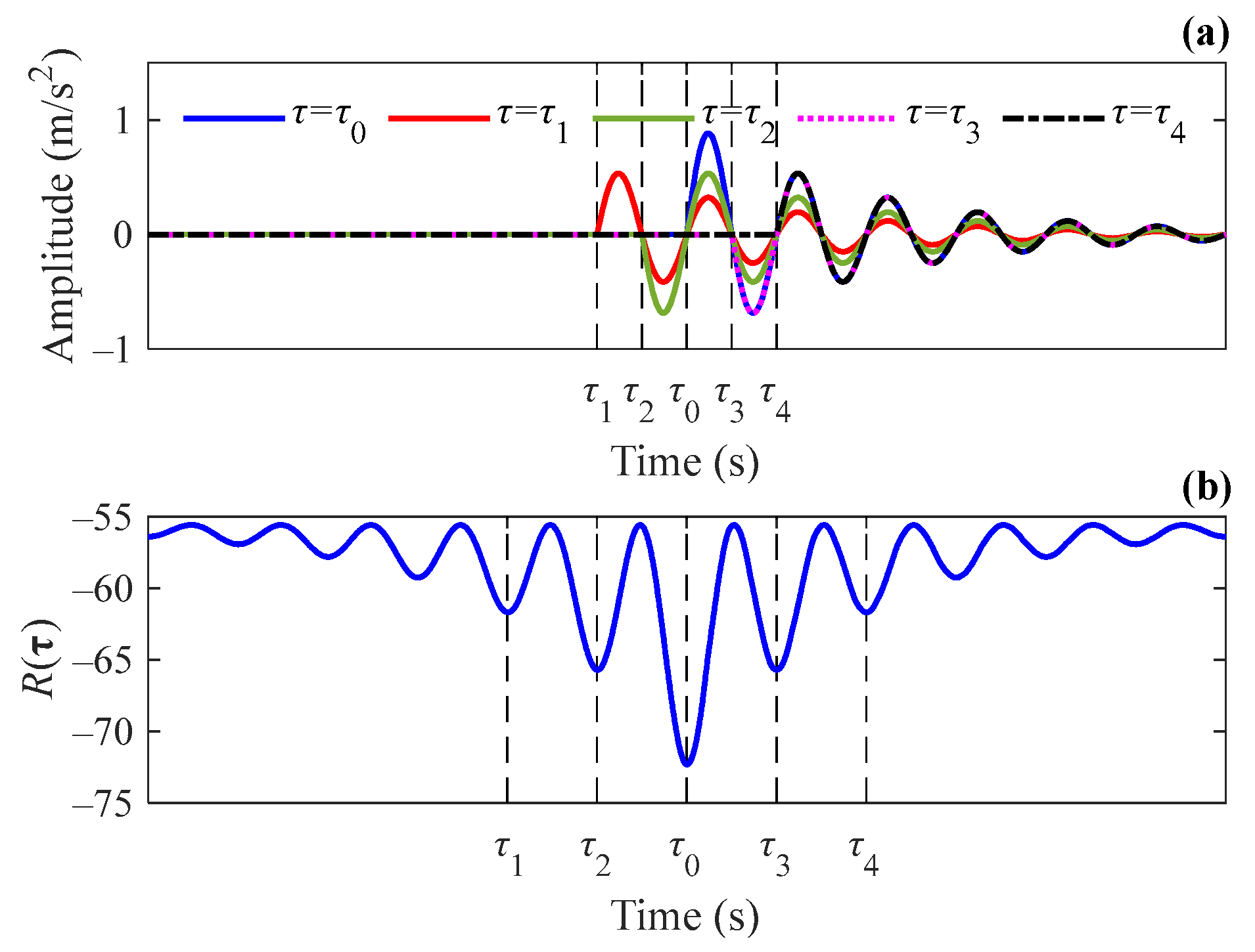
3.2. Construction and Optimization of the Surrogate Function
3.3. Sparsity-Enhanced Optimization and Fidelity-Enhanced Optimization
| Algorithm 1. Pseudo-code of the SSR Algorithm |
| Input: vibration signal: , initial time index: , sparse dictionary: , parameters: , , Initialize: , Repeat (1) Construct the surrogate function construct by Equation (9) (2) Optimize the surrogate function For , do update by Equations (11), (13) and (14) update by Equation (4) End for (3) Update the regularization parameter and prune the time index variables update by Equations (12) and (16) If , update by Equation (18); else, set ; end if For , do If , set ; set ; end if End for Until Return |
4. Simulation Analysis and Parameter Setting
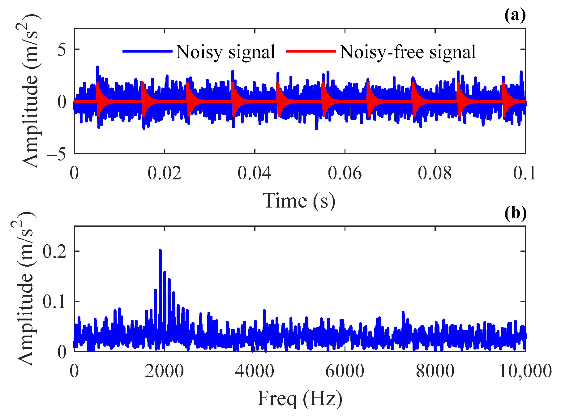
4.1. Generating Simulation Signals
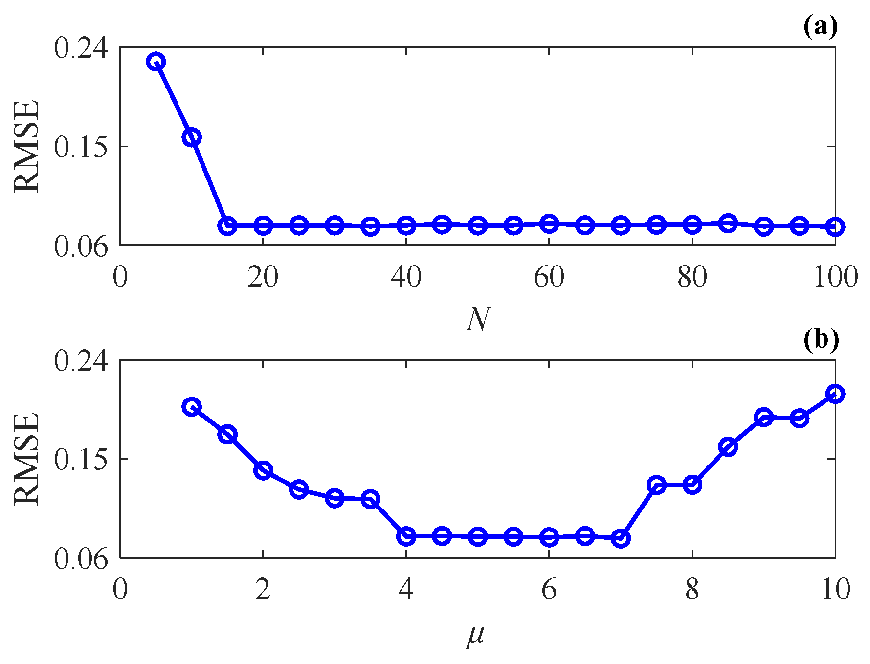
4.2. Parameter Setting for the SSR Method
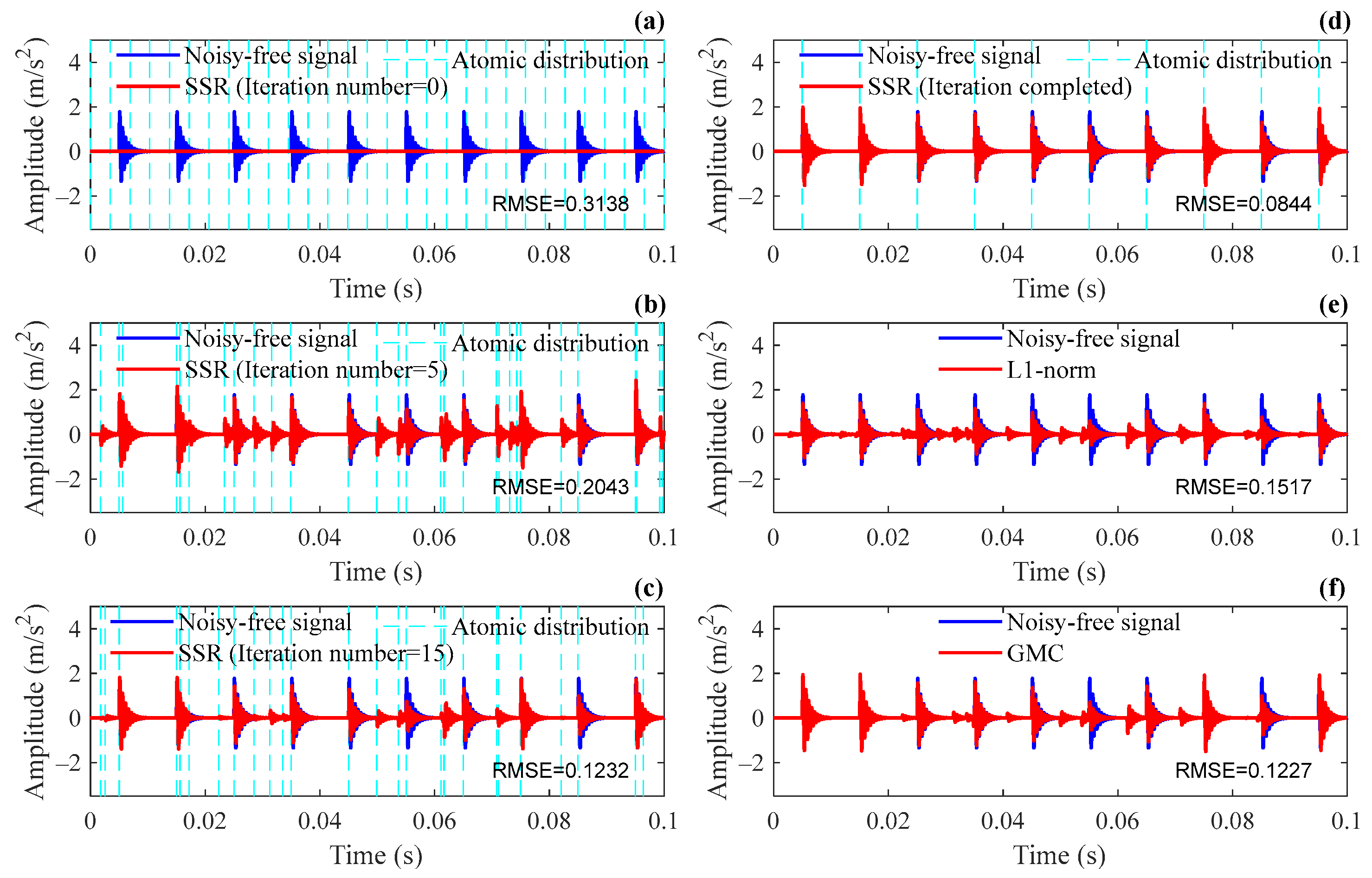
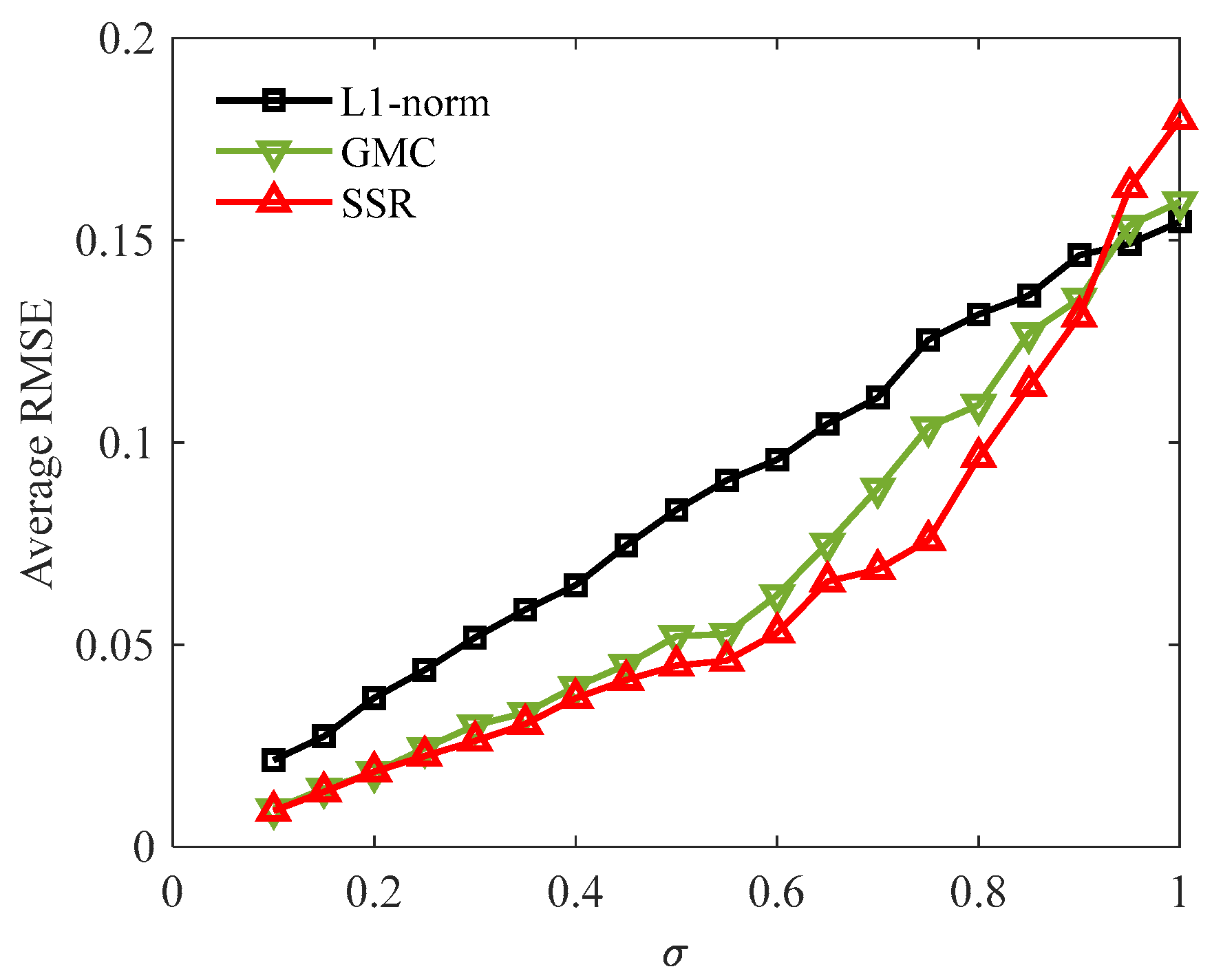
4.3. Simulation Analysis
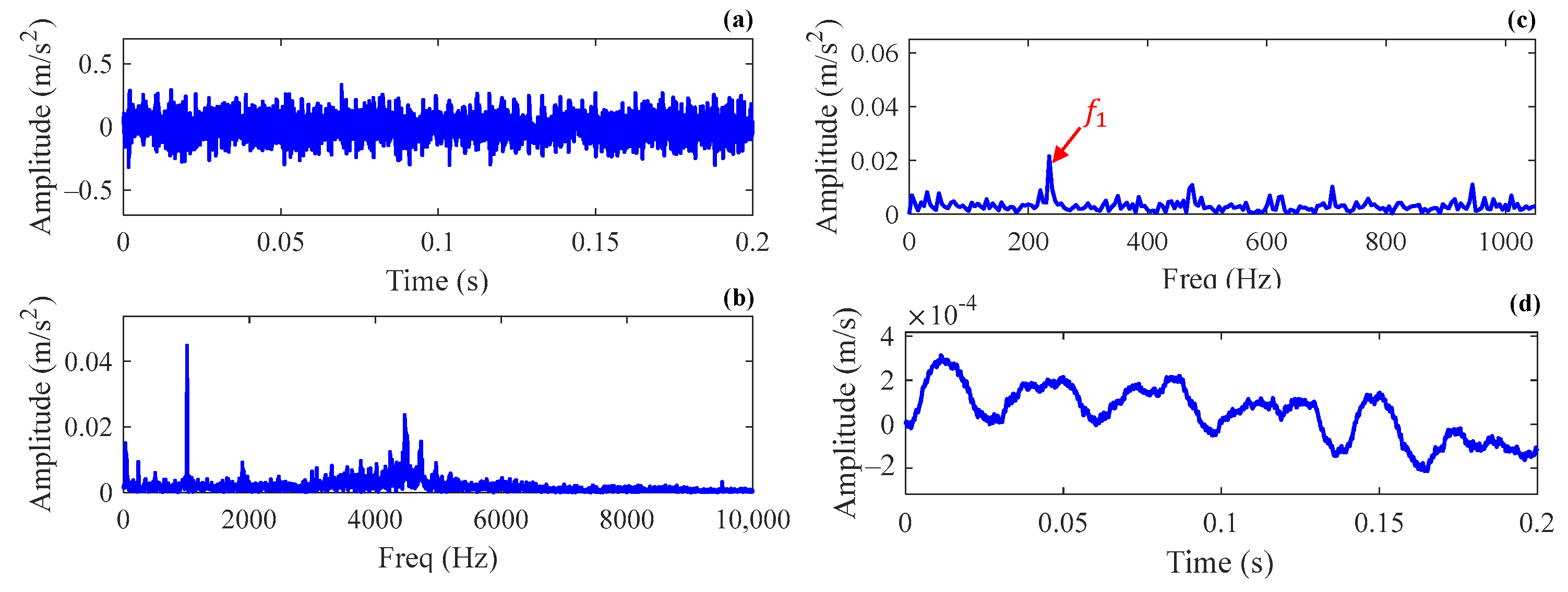
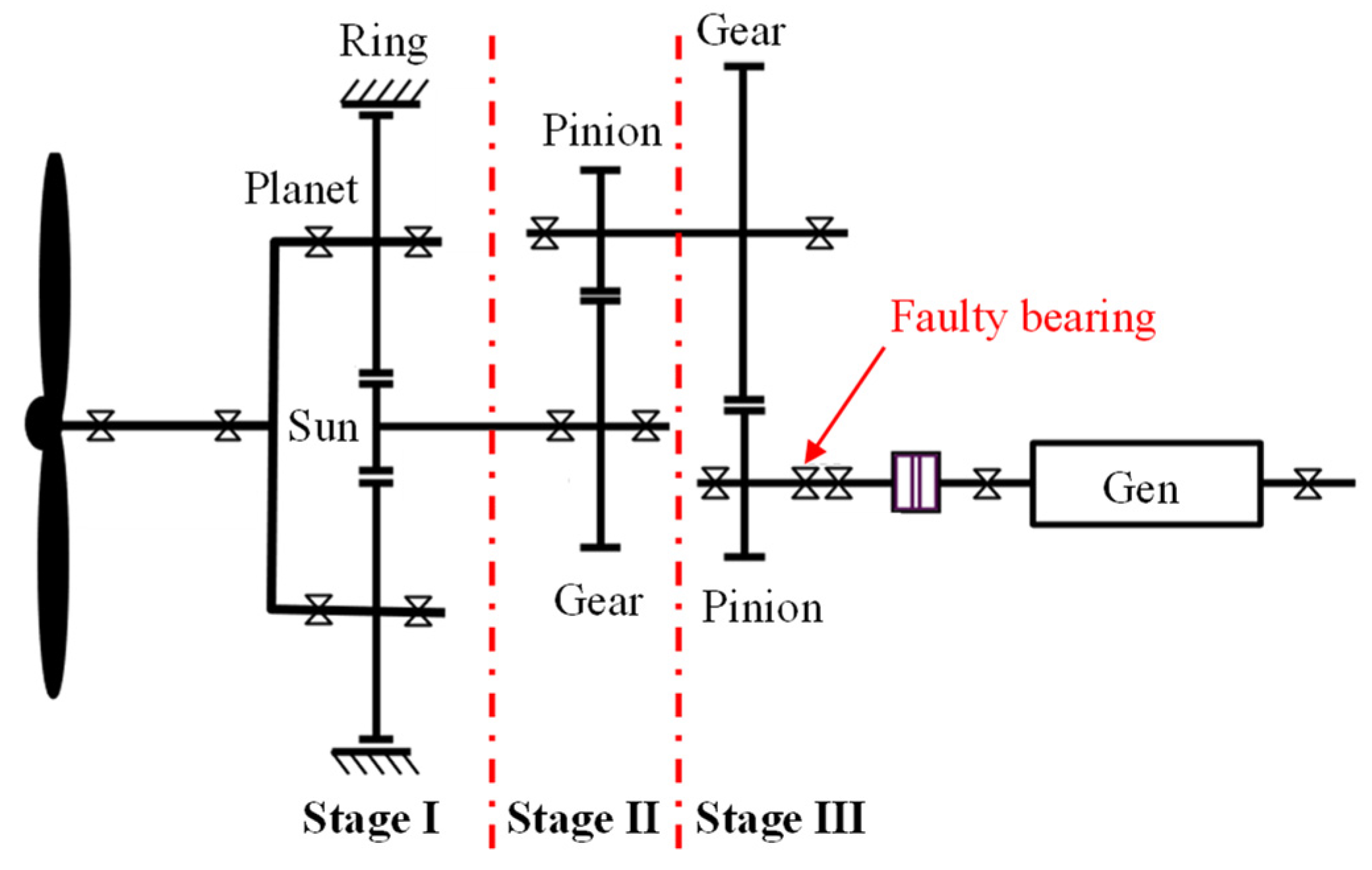
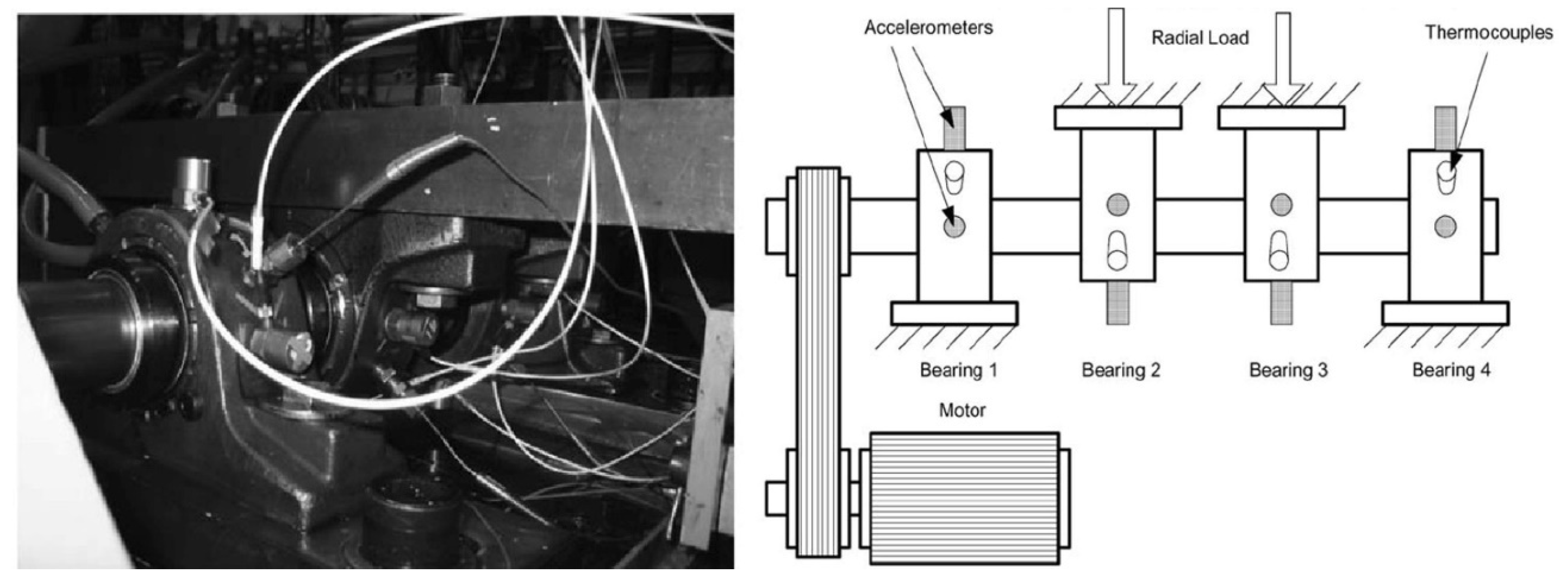
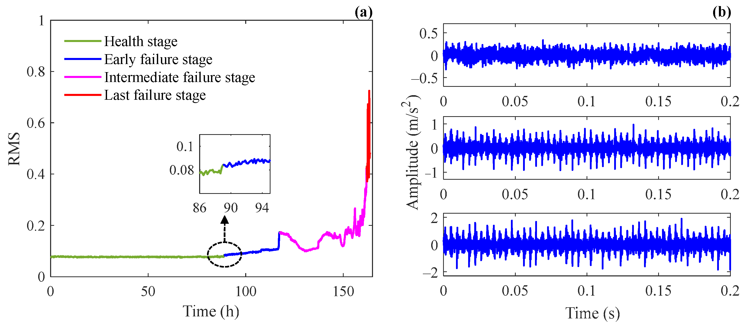
5. Experimental Verifications
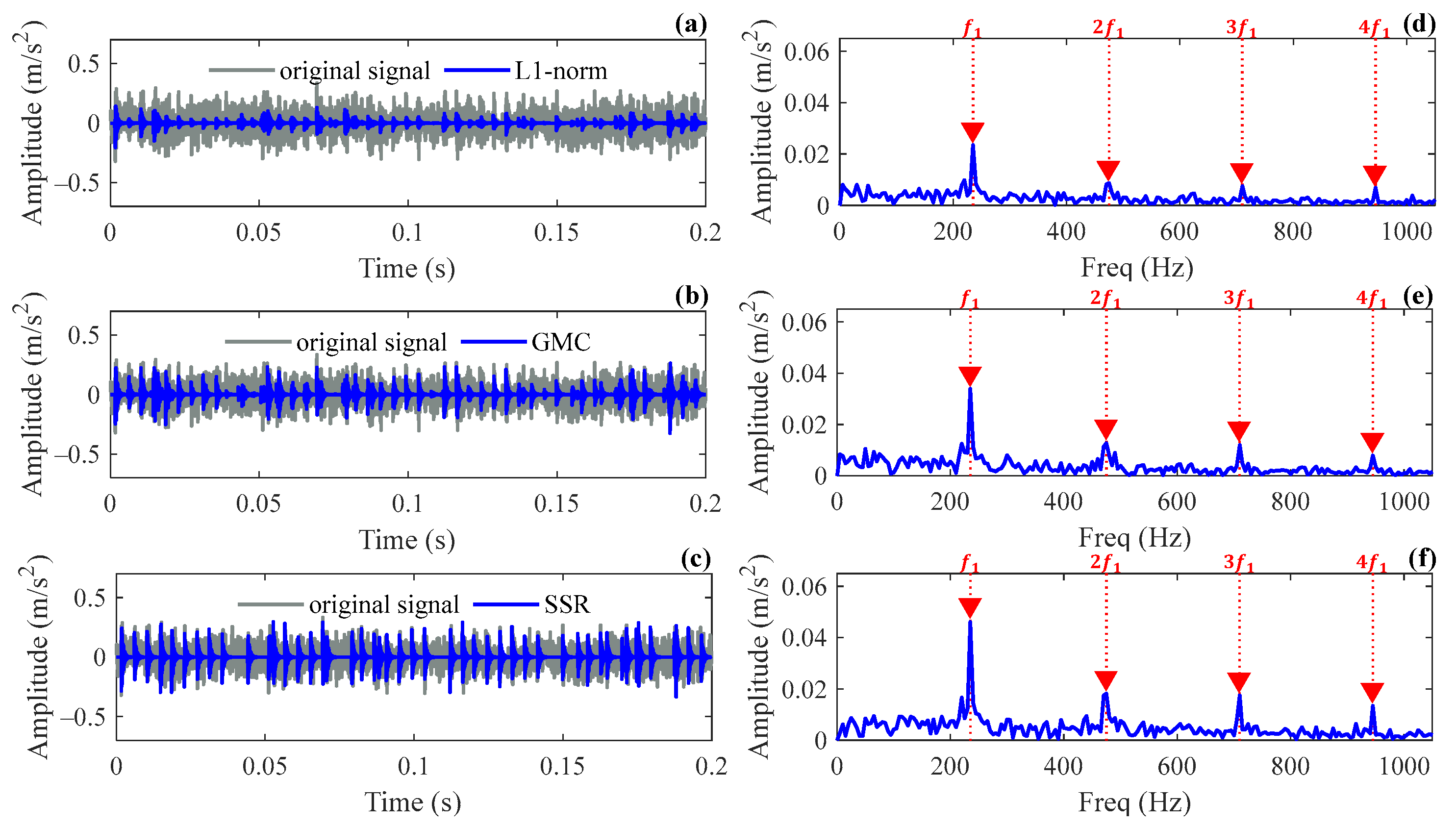
5.1. Case 1
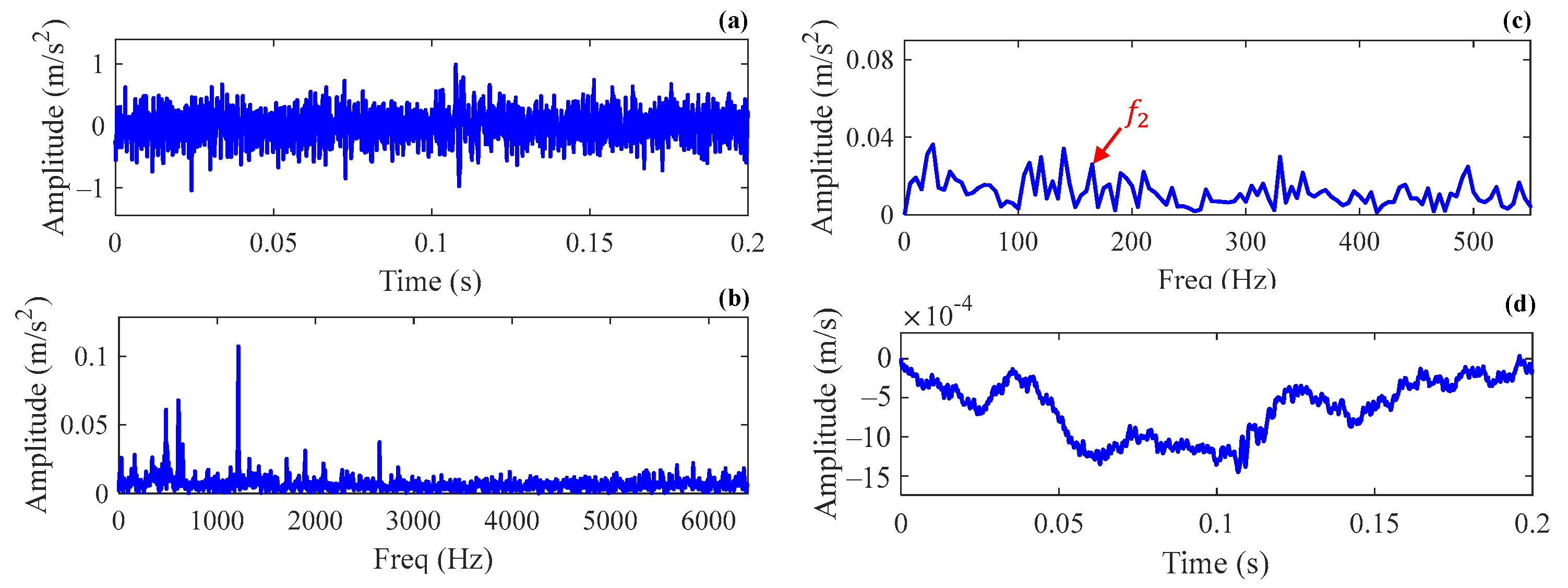
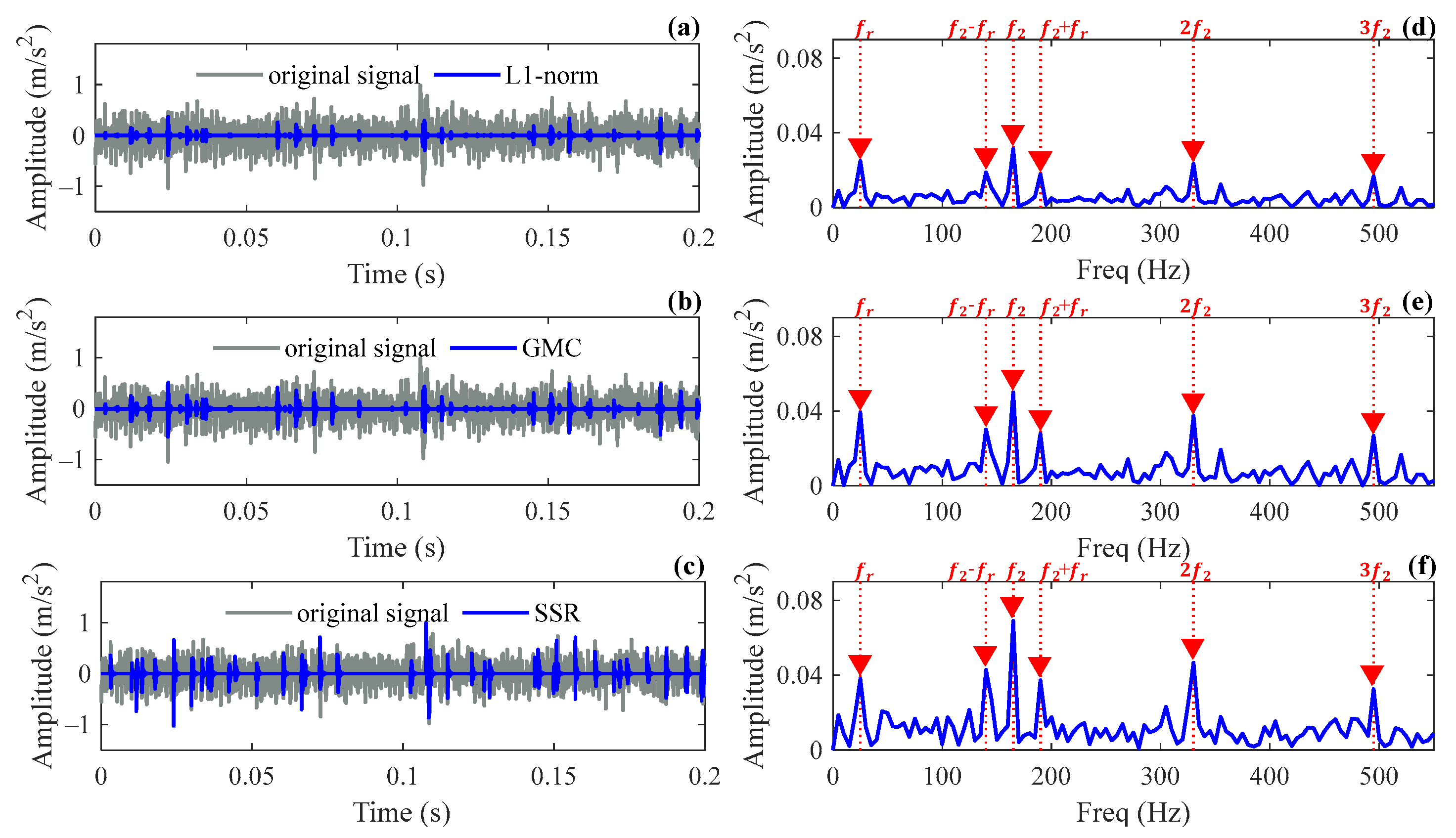
5.2. Case 2
6. Conclusions
Author Contributions
Funding
Institutional Review Board Statement
Informed Consent Statement
Data Availability Statement
Conflicts of Interest
References
- Randall, R.B.; Antoni, J. Rolling element bearing diagnostics—A tutorial. Mech. Syst. Signal. Process. 2011, 25, 485–520. [Google Scholar] [CrossRef]
- Gradzki, R.; Bartoszewicz, B.; Martinez, J.E. Bearing Fault Diagnostics Based on the Square of the Amplitude Gains Method. Appl. Sci. 2023, 13, 2160. [Google Scholar] [CrossRef]
- Chen, R.X.; Tang, L.L.; Hu, X.L.; Wu, H.N.A. Fault Diagnosis Method of Low-Speed Rolling Bearing Based on Acoustic Emission Signal and Subspace Embedded Feature Distribution Alignment. IEEE Trans. Ind. Inform. 2021, 17, 5402–5410. [Google Scholar] [CrossRef]
- Liu, Z.P.; Yang, B.Y.; Wang, X.F.; Zhang, L. Acoustic Emission Analysis for Wind Turbine Blade Bearing Fault Detection Under Time-Varying Low-Speed and Heavy Blade Load Conditions. IEEE Trans. Ind. Appl. 2021, 57, 2791–2800. [Google Scholar] [CrossRef]
- Qiu, Y.; Tan, B.; Li, D.; Jiang, H.; Feng, Y. Thermal analysis of rolling bearing at wind turbine gearbox high speed end. In Proceedings of the International Conference on Renewable Power Generation (RPG 2015), Beijing, China, 17–18 October 2015. [Google Scholar]
- Chen, B.; Yin, P.; Gao, Y.; Peng, F.Y. Use of the correlated EEMD and time-spectral kurtosis for bearing defect detection under large speed variation. Mech. Mach. Theory 2018, 129, 162–174. [Google Scholar] [CrossRef]
- Li, Y.; Zhou, J.W.; Li, H.G.; Meng, G.; Bian, J. A Fast and Adaptive Empirical Mode Decomposition Method and Its Application in Rolling Bearing Fault Diagnosis. IEEE Sens. J. 2023, 23, 567–576. [Google Scholar] [CrossRef]
- Li, J.M.; Cheng, X.; Li, Q.; Meng, Z. Adaptive energy-constrained variational mode decomposition based on spectrum segmentation and its application in fault detection of rolling bearing. Signal Process. 2021, 183, 108025. [Google Scholar] [CrossRef]
- Wang, H.B.; Yang, T.G.; Han, Q.K.; Luo, Z. Approach to the Quantitative Diagnosis of Rolling Bearings Based on Optimized VMD and Lempel-Ziv Complexity under Varying Conditions. Sensors 2023, 23, 4044. [Google Scholar] [CrossRef] [PubMed]
- Antoni, J. The spectral kurtosis: A useful tool for characterising non-stationary signals. Mech. Syst. Signal. Process. 2006, 20, 282–307. [Google Scholar] [CrossRef]
- Wang, D. Some further thoughts about spectral kurtosis, spectral L2/L1 norm, spectral smoothness index and spectral Gini index for characterizing repetitive transients. Mech. Syst. Signal. Process. 2018, 108, 360–368. [Google Scholar] [CrossRef]
- Yan, R.Q.; Gao, R.X.; Chen, X.F. Wavelets for fault diagnosis of rotary machines: A review with applications. Signal Process. 2014, 96, 1–15. [Google Scholar]
- Hong, H.B.; Liang, M. Fault severity assessment for rolling element bearings using the Lempel-Ziv complexity and continuous wavelet transform. J. Sound Vib. 2009, 320, 452–468. [Google Scholar] [CrossRef]
- Chen, X.F.; Cai, G.G.; Cao, H.R.; Xin, W. Condition assessment for automatic tool changer based on sparsity-enabled signal decomposition method. Mechatronics 2015, 31, 50–59. [Google Scholar] [CrossRef]
- Feng, Z.P.; Zhou, Y.K.; Zuo, M.J.; Chu, F.L.; Chen, X.W. Atomic decomposition and sparse representation for complex signal analysis in machinery fault diagnosis: A review with examples. Measurement 2017, 103, 106–132. [Google Scholar] [CrossRef]
- He, W.P.; Ding, Y.; Zi, Y.Y.; Selesnick, I.W. Sparsity-based algorithm for detecting faults in rotating machines. Mech. Syst. Signal. Process. 2016, 72–73, 46–64. [Google Scholar] [CrossRef]
- Zheng, K.; Li, T.L.; Su, Z.Q.; Zhang, B. Sparse Elitist Group Lasso Denoising in Frequency Domain for Bearing Fault Diagnosis. IEEE Trans. Ind. Inform. 2021, 17, 4681–4691. [Google Scholar] [CrossRef]
- Liao, Y.; Huang, W.; Shen, C.; Zhu, Z.; Xuan, J.; Mao, L. Enhanced Sparse Regularization Based on Logarithm Penalty and Its Application to Gearbox Compound Fault Diagnosis. IEEE Trans. Instrum. Meas. 2021, 70, 1–12. [Google Scholar] [CrossRef]
- Sun, Y.H.; Yu, J.B. Adaptive k-Sparsity-Based Weighted Lasso for Bearing Fault Detection. IEEE Sens. J. 2022, 22, 4326–4337. [Google Scholar] [CrossRef]
- Wang, H.Q.; Ke, Y.L.; Song, L.Y.; Tang, G.; Chen, P. A Sparsity-Promoted Decomposition for Compressed Fault Diagnosis of Roller Bearings. Sensors 2016, 16, 1524. [Google Scholar] [CrossRef]
- Zheng, K.; Bai, Y.; Xiong, J.F.; Tan, F.; Yang, D.W.; Zhang, Y. Simultaneously Low Rank and Group Sparse Decomposition for Rolling Bearing Fault Diagnosis. Sensors 2020, 20, 5541. [Google Scholar] [CrossRef] [PubMed]
- Chen, S.S.; Donoho, D.L.; Saunders, M.A. Atomic decomposition by basis pursuit. SIAM Rev. 2001, 43, 129–159. [Google Scholar] [CrossRef]
- Selesnick, I. Sparse Regularization via Convex Analysis. IEEE Trans. Signal Process. 2017, 65, 4481–4494. [Google Scholar] [CrossRef]
- Wang, S.; Selesnick, I.; Cai, G.; Feng, Y.; Sui, X.; Chen, X. Nonconvex Sparse Regularization and Convex Optimization for Bearing Fault Diagnosis. IEEE Trans. Ind. Electron. 2018, 65, 7332–7342. [Google Scholar] [CrossRef]
- He, W.; Hu, J.; Chen, B.; Guo, B. GMC sparse enhancement diagnostic method based on the tunable Q-factor wavelet transform for detecting faults in rotating machines. Measurement 2021, 174, 109001. [Google Scholar] [CrossRef]
- Huang, W.; Song, Z.; Zhang, C.; Wang, J.; Shi, J.; Jiang, X.; Zhu, Z. Multi-source fidelity sparse representation via convex optimization for gearbox compound fault diagnosis. J. Sound Vib. 2021, 496, 115879. [Google Scholar] [CrossRef]
- Fang, J.; Wang, F.Y.; Shen, Y.N.; Li, H.B.; Blum, R.S. Super-Resolution Compressed Sensing for Line Spectral Estimation: An Iterative Reweighted Approach. IEEE Trans. Signal Process. 2016, 64, 4649–4662. [Google Scholar] [CrossRef]
- Lange, K.; Hunter, D.R.; Yang, I. Optimization transfer using surrogate objective functions. J. Comput. Graph. Stat. 2000, 9, 1–20. [Google Scholar]
- Sun, Y.; Babu, P.; Palomar, D.P. Majorization-Minimization Algorithms in Signal Processing, Communications, and Machine Learning. IEEE Trans. Signal Process. 2017, 65, 794–816. [Google Scholar] [CrossRef]
- Donoho, D.L. For most large underdetermined systems of linear equations the minimal l(1)-norm solution is also the sparsest solution. Commun. Pur. Appl. Math. 2006, 59, 797–829. [Google Scholar] [CrossRef]
- Natarajan, B.K. Sparse Approximate Solutions to Linear-Systems. SIAM J. Comput. 1995, 24, 227–234. [Google Scholar] [CrossRef]
- Wang, S.B.; Huang, W.G.; Zhu, Z.K. Transient modeling and parameter identification based on wavelet and correlation filtering for rotating machine fault diagnosis. Mech. Syst. Signal. Process. 2011, 25, 1299–1320. [Google Scholar] [CrossRef]
- He, G.L.; Ding, K.; Lin, H.B. Gearbox coupling modulation separation method based on match pursuit and correlation filtering. Mech. Syst. Signal. Process. 2016, 66–67, 597–611. [Google Scholar] [CrossRef]
- Tipping, M.E. Sparse Bayesian learning and the relevance vector machine. J. Mach. Learn. Res. 2001, 1, 211–244. [Google Scholar]
- Ji, S.H.; Xue, Y.; Carin, L. Bayesian compressive sensing. IEEE Trans. Signal Process. 2008, 56, 2346–2356. [Google Scholar] [CrossRef]
- Qiu, H.; Lee, J.; Lin, J.; Yu, G. Wavelet filter-based weak signature detection method and its application on rolling element bearing prognostics. J. Sound Vib. 2006, 289, 1066–1090. [Google Scholar] [CrossRef]


| Method | L1-Norm | GMC | SSR |
|---|---|---|---|
| Average time cost | 22.1 s | 195.1 s | 71.4 s |
| Method | L1-Norm | GMC | SSR |
|---|---|---|---|
| 163 | 163 | 48 | |
| 0.0235 | 0.0339 | 0.0461 |
| Parameters | Value |
|---|---|
| No. of rolling elements | 12 |
| Inside diameter (mm) | 140 |
| Outside diameter (mm) | 300 |
| Thickness (mm) | 62 |
| Pitch diameter (mm) | 220 |
| Roller diameter (mm) | 47.4 |
| Contact angle (deg) | 35 |
| Fault characteristic coefficient for inner race | 7.06 |
| Method | L1-Norm | GMC | SSR |
|---|---|---|---|
| 101 | 101 | 49 | |
| 0.0313 | 0.0499 | 0.0691 | |
| 0.0189 | 0.0301 | 0.0429 | |
| 0.0178 | 0.0279 | 0.0373 |
Disclaimer/Publisher’s Note: The statements, opinions and data contained in all publications are solely those of the individual author(s) and contributor(s) and not of MDPI and/or the editor(s). MDPI and/or the editor(s) disclaim responsibility for any injury to people or property resulting from any ideas, methods, instructions or products referred to in the content. |
© 2024 by the authors. Licensee MDPI, Basel, Switzerland. This article is an open access article distributed under the terms and conditions of the Creative Commons Attribution (CC BY) license (https://creativecommons.org/licenses/by/4.0/).
Share and Cite
Yu, L.; Wang, C.; Zhang, F.; Luo, H. Bearing Fault Diagnosis via Stepwise Sparse Regularization with an Adaptive Sparse Dictionary. Sensors 2024, 24, 2445. https://doi.org/10.3390/s24082445
Yu L, Wang C, Zhang F, Luo H. Bearing Fault Diagnosis via Stepwise Sparse Regularization with an Adaptive Sparse Dictionary. Sensors. 2024; 24(8):2445. https://doi.org/10.3390/s24082445
Chicago/Turabian StyleYu, Lichao, Chenglong Wang, Fanghong Zhang, and Huageng Luo. 2024. "Bearing Fault Diagnosis via Stepwise Sparse Regularization with an Adaptive Sparse Dictionary" Sensors 24, no. 8: 2445. https://doi.org/10.3390/s24082445
APA StyleYu, L., Wang, C., Zhang, F., & Luo, H. (2024). Bearing Fault Diagnosis via Stepwise Sparse Regularization with an Adaptive Sparse Dictionary. Sensors, 24(8), 2445. https://doi.org/10.3390/s24082445