Abstract
The accurate measurement and the investigation of electromagnetic transients are becoming more important, especially with the increasing integration of renewable energy sources into the power grid. These sources introduce new transient phenomena due to the extensive use of power electronics. To achieve this, the measurement devices must have a broadband response capable of measuring fast transients. This paper presents a capacitive electric field sensor-based measurement system to measure transient overvoltages in high-voltage substations. The concept and design of the measurement system are first presented. Then, the design and concept are validated using tests performed in a high-voltage laboratory. Afterwards, two different calibration techniques are discussed: the simplified method (SM) and the coupling capacitance compensation (CCC) method. Finally, three recorded transients are evaluated using the calibration methods. The investigation revealed that the SM tends to overestimate the maximum overvoltage, highlighting the CCC method as a more suitable approach for calibrating transient overvoltage measurements. This measurement system has been validated using various measurements and can be an efficient and flexible solution for the long-term monitoring of transient overvoltages in high-voltage substations.
1. Introduction
Transient overvoltage events are one of the major causes of dielectric failures in substation equipment [1,2]. These events are caused by switching operations, lightning discharges, and short circuits, among others [3]. With the increasing integration of renewable energy sources into the electric power system, the system dynamics are changing, and new transient phenomena are occurring [4,5,6]. Investigating their effects on substation equipment and accurately measuring the transients becomes even more important.
The required frequency bandwidth of the measuring device depends on the transient being measured. In high-voltage substations, voltage measurement is often carried out using capacitive voltage transformers (CVT) or inductive voltage transformers (IVT). Although these devices provide accurate measurements at nominal frequency, their outputs deviate significantly at higher frequencies [7,8,9,10,11]. Consequently, this characteristic restricts their application for measuring fast transients.
To overcome the limitations of voltage transformers, specific techniques have been proposed in the literature [10,11,12,13,14,15,16]. Most of these methods focus on correcting the distorted output voltage. However, these approaches often require complex filtering techniques or the installation of additional devices. Another strategy to measure transients is to use voltage sensors connected to the measurement tap of transformer bushings [17,18,19,20,21]. While this technique has high accuracy and wide bandwidth, its use is limited to transformer bays.
Using electric field sensors for voltage measurement is another solution that has been the subject of research and further improvement [22,23,24,25,26,27,28,29,30,31,32,33]. In [25,26,27,28], the authors propose voltage calculation through inversion or integration of the measured electric field. However, these methods require complex algorithms to solve matrix inverse operations or numerical integration of the spatial electric field. This results in low accuracy and long computation time [25,28]. In [29], the voltage is calculated from the rate of change in the electric displacement field, using a differential self-integration D-dot sensor. However, this sensor is a near-field device positioned on the ceramic casing of the conductor, exhibiting inflexibility and a potential galvanic risk. Another investigated technique involves voltage measurement based on a differentiating/integrating (D/I) concept [30,31,32], utilizing a capacitive pick-up electrode composed of a parallel plate capacitor with a grounded bottom plate. The primary drawback of this method is its low accuracy due to the neglect or inaccurate estimation of coupling between the outer phases. In [33], various alternative methods for measuring transients using unconventional transducers are discussed. One of these methods employs a coupling plane as an electric field sensor; however, the author provides only a brief overview of the technique.
This paper presents a measurement system based on capacitive electric field sensors to measure transient overvoltages in a high-voltage substation. Two prior publications [34,35] have briefly outlined the system’s concept, major components, and its field application. In [34], the measurement system monitored switching transient overvoltages during the energization of a 420 kV transmission line. The primary aim was to investigate the failure of a surge arrester during a switching operation. In [35], the authors evaluated some measured transient overvoltages in the frequency domain. The analysis revealed that the transients contain significant high-frequency components (>>1 kHz), making traditional IVT or CVT unsuitable for accurately measuring them.
This study extensively discusses the concept and design of the measurement system, introduces an improved calibration method, and provides a statistical analysis of signals measured during a one-year measurement campaign. Section 2 outlines the system’s concept and design. Section 3 reports the results of the validation performed in a high-voltage laboratory. Section 4 describes the aspects of the measurement system installation in a high-voltage substation and discusses two calibration methods. Section 5 presents the statistical analysis of all recorded transients and evaluates three of them using the different calibration methods. Finally, Section 6 presents the conclusions of the study.
2. Concept and Design of the Measurement System
A measurement system based on capacitive electric field sensors has been developed to measure transient overvoltages in substations. Figure 1 shows its schematic diagram.
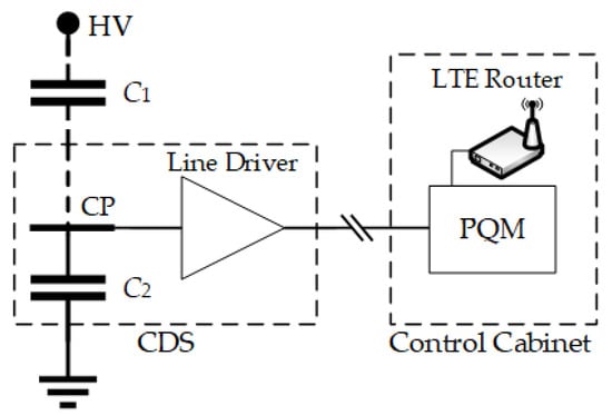
Figure 1.
Schematic diagram of the transient overvoltage measurement system.
The capacitance C1 represents the stray capacitance between the coupling plane (CP) and the high-voltage connection (HV) if the measurement device is installed under a substation busbar or on the base of a disconnector (see Figure 2). The user-defined capacitance C2 is connected between CP and ground and is chosen based on the desired voltage ratio. There is also a stray capacitance between the CP and ground (around 30 pF), but it is much smaller than C2 and can be neglected. Therefore, considering both capacitances C1 and C2, the measurement system has a capacitive divider whose voltage ratio is given by:
where Vin is the voltage between HV and ground, and Vout is the divider’s output voltage.
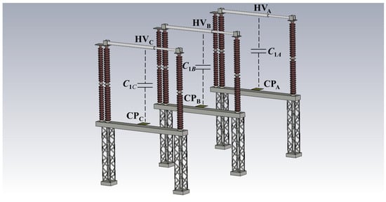
Figure 2.
Three-dimensional model of the measurement setup for calculation of stray capacitance C1.
Equation (1) is used to calculate the expected voltage ratio, considering the maximum voltage expected in a transient overvoltage (Vin-max) and the maximum output voltage suitable for the measurement system (Vout-max). In this study, Vin-max is considered as 1 MV and Vout-max as 20 V. Thus, the theoretical voltage ratio is 50,000:1. To accurately determine this voltage ratio, the capacitances C1 and C2 must be known. However, C1 is a stray capacitance that changes according to the layout where the measurement system is installed. Therefore, this capacitance is estimated using the finite element method (FEM) in CST Studio Suite® version 2021 [36]. The three-dimensional model of the setup is shown in Figure 2.
The three sensors are installed, one on each base of a three-phase disconnector. The electric field can be assumed to be quasi-static considering the steady-state voltage. As a result, it exhibits the characteristics of an electrostatic field [25]. Therefore, the stray capacitance C1 is calculated using the electrostatic solver in CST Studio.
The CST Studio model uses the technical drawing of the substation as the reference. The distance between phases is 4.50 m. The disconnector base is made of metal and has a height of 2.75 m. The moving contact of the disconnector is 3.75 m long and has a radius of 0.05 m. The insulators are modeled as ceramic porcelain with a relative permittivity ε = 6, a relative permeability μ = 1, a height of 3.35 m, and an outer radius of 0.13 m. The sensor’s CP is 0.10 m above the base of the disconnector. It has a length, width, and height of 0.40 m, 0.40 m, and 0.04 m, respectively. All the metal parts are modeled as perfect electric conductors (PEC), with the voltage of the moving contact set at 242.5 kV. The sensors and bases are grounded.
According to the electrostatic simulation, the calculated capacitances, C1B, and C1C are 0.766 pF, 0.772 pF, and 0.776 pF, respectively. The difference between C1A and C1C arises from the inherent approximation within the FEM. To achieve a voltage ratio of 50,000:1, the capacitance C2 should be 38.6 nF, based on the average of the calculated C1 values. Additionally, there is a coupling between each sensor and the adjacent phases. This topic will be discussed in Section 4.
2.1. The Capacitive Divider Setup
After estimating the capacitance C1 and defining the voltage divider requirements, the capacitive divider setup (CDS) is designed and assembled. The CDS comprises a CP and an electronic circuit mounted in an IP65 metal enclosure. The CP is an aluminum plate connected to the electronic circuit through an external terminal. Figure 3 shows the CP (a) and the metal housing (b) of the electronic circuit. The housing has four external connectors: one 4 mm connector for the CP, one N-connector for the measurement coaxial cable, one waterproof 2-pin connector for the DC source, and one ground connector.
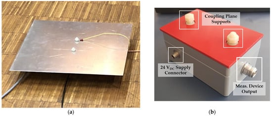
Figure 3.
External components of the CDS. (a) Coupling plane; (b) metal housing with connections.
Inside the metal housing, the CP connects to the capacitors constituting C2. Specifically, six 8.3 nF temperature-stable SMD capacitors are connected in parallel to achieve a capacitance of 49.8 nF. If the output of the voltage divider is directly connected to a measurement instrument using a long coaxial cable, the cable’s capacitance influences the voltage ratio of the measurement system. Consequently, a line driver is employed to decouple the capacitive divider from the coaxial measurement cable.
The line driver uses a JFET input operational amplifier [37] with a slew rate of 60 V/µs, a bandwidth of 14 MHz, and a supply voltage of ±20 V. The circuit board also has additional internal buffered converters [38] to ensure voltage stability. A 15 m coaxial cable connects the line driver output to a power quality monitor. Figure 4 shows the electronic circuit of the CDS (a) and the six parallel capacitors of C2 (b).
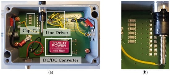
Figure 4.
Electronic circuit of the CDS. (a) Top view; (b) parallel capacitors of C2.
2.2. The Power Quality Monitor
A power quality monitor [39] is installed in a control cabinet to read and record the measured transient signals. It measures high-frequency harmonics and transients at a sampling rate of 1 MS/s. It has eight channels with synchronous sampling: four channels with 4 mm connectors with an input impedance of 10 MΩ and an input range from −600 V to +600 V; and four channels with BNC connectors with an input impedance of 1 MΩ and an input range from −50 V to +50 V. The transients recorded by the power quality monitor PQM-800 are stored internally and can also be uploaded to a monitoring cloud.
The control cabinet also includes an LTE router for sending the recorded transients to the monitoring cloud and a 24 V DC power supply for the CDS, as shown in Figure 5.
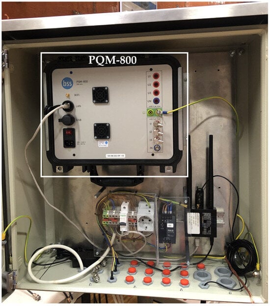
Figure 5.
The control cabinet with the power quality monitor.
3. Tests in the High-Voltage Laboratory
Three CDSs are assembled for monitoring transient overvoltages in the substation. Prior to installation, the devices are tested in the high-voltage laboratory of the University of Stuttgart, where the following tests are conducted:
- Measurement of C2 capacitances;
- Accuracy assessment (measurement of divider ratio and stray capacitances C1);
- Lightning impulse test;
- Measurement of the CDS bandwidth.
The capacitances C2 of the CDSs, formed by temperature-stable multilayer ceramic capacitors (MLCC), are measured using a multimeter. The values obtained for the devices MD1, MD2, and MD3 are 49.94 nF, 50.76 nF, and 50.53 nF, respectively.
3.1. Accuracy Assessment Using AC Voltage
The accuracy of the three CDSs is assessed by measuring the voltage ratio and the stray capacitance C1 of the setup built in the high-voltage laboratory. Despite differences from the configuration in Figure 2, it is still possible to evaluate the linearity of the measurement system response since C1 is the only parameter that changes based on the layout. The measurements are performed individually with an input voltage range from 13 kVrms to 76 kVrms. Figure 6 shows the schematic diagram (a) and the setup (b) for measuring the accuracy of the CDSs.
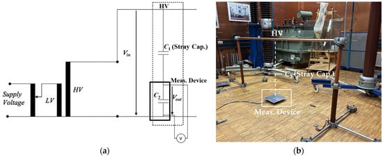
Figure 6.
Measurement of the accuracy of the CDSs. (a) Schematic diagram; (b) test setup.
The input high voltage Vin is measured using a standard capacitive divider with a ratio of 3060:1. Both signals, the output of the standard divider and the output of the CDSs (Vout), are evaluated with a 70 MHz oscilloscope with a sampling rate of 1 GS/s. The stray capacitance C1 is then calculated from Equation (1) using the measured values of C2, Vin, and Vout. Figure 7 shows the measured values of voltage ratio (a) and stray capacitance C1 (b). Ten measurements are conducted for each device, with the input voltage ranging from 13 kVrms to 76 kVrms.
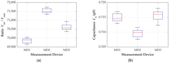
Figure 7.
Measurement results. (a) Voltage ratio; (b) stray capacitance C1.
The median voltage ratios for devices MD1, MD2, and MD3 are 69,892:1, 71,503:1, and 70,574:1, respectively. The average voltage ratios are 69,859:1, 71,535:1, and 70,610:1. Distinct voltage ratios are expected due to the dependence of the ratio on C1 and C2 and the different capacitances C2 among the CDSs.
The stray capacitance C1 should ideally have a unique value for a given configuration. However, variations are observed in the measurements of the three units, potentially attributed to sensor sensitivity or slight misalignment of the devices during measurements. Considering the average value of C1 for each unit, the maximum error observed is 0.29% for devices MD1 and MD2, and 0.46% for device MD3.
The accuracy of the measurement devices is assessed by analyzing the voltage ratio measured for each device. The ratio error is calculated as follows:
where kr is the average of the measured voltage ratios for each device. The results are given in Table 1, which shows a linear behavior of the measurement devices concerning the applied voltage. The maximum error observed is 0.29% for devices MD1 and MD2, and 0.46% for device MD3, relative to their average voltage ratios.

Table 1.
Ratio error considering the average of the measured voltage ratios.
3.2. Lightning Impulse Test
The lightning impulse test is the next evaluation performed in the high-voltage laboratory. The standard IEC 60060-1 [40] defines a lightning impulse as a double exponential waveform characterized by a front time T1 of 1.2 µs ±30% and a tail time T2 of 50 µs ±20%. The impulse generator can deliver switching and lightning impulse voltages up to 1 MV and a total energy of 30 kJ. Figure 8 illustrates the schematic diagram (a) and test setup (b).
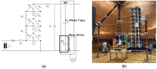
Figure 8.
Lightning impulse test. (a) Schematic diagram; (b) test setup.
The applied impulse voltage is measured using a standard capacitive divider. Its output and the output from device MD1 are evaluated using an oscilloscope with a bandwidth of 1 GHz and a sampling rate of 10 GS/s. Figure 9 shows the measurement of the lightning impulse, where the output voltage from unit MD1 is multiplied by the voltage ratio measured for this configuration, which is 20,434:1.
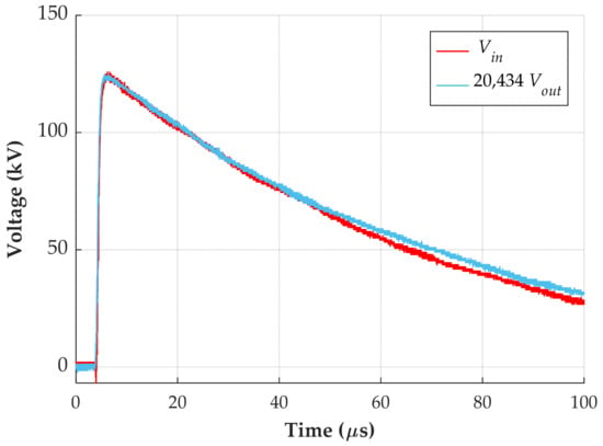
Figure 9.
Lightning impulse response of device MD1.
The applied lightning impulse has a front time of 1.22 µs and a tail time of 51.48 µs, whereas device MD1 exhibits a front time of 1.17 µs and a tail time of 54.35 µs. Both signals meet the criteria of IEC 60060-1 and demonstrate similarity. Therefore, the measurement device can accurately reproduce a lightning impulse signal.
3.3. Measurement of the CDS Bandwidth
The measurement of the CDS bandwidth is performed using a 120 pF ceramic capacitor to simulate the stray capacitance C1. Although the typical stray capacitance is less than 1 pF, a higher value is chosen to improve the signal-to-noise ratio of the measurement. Using a Rohde & Schwarz ZVRE vector network analyzer (VNA) [41] with a frequency range from 9 kHz to 4 GHz, the measurement assessed the Vout/Vin ratio over a frequency range spanning from 10 kHz to 10 MHz. Figure 10 shows the test setup (a) and the obtained measurement results (b).
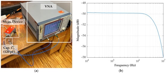
Figure 10.
Bandwidth measurement of device MD1. (a) Test setup; (b) measurement result.
The frequency response measurement shows a constant ratio of −49.8 dB up to 1.2 MHz, with the 3 dB frequency at 5.6 MHz. It indicates that the measurement device has a broadband response and can measure fast transients. However, the power quality monitor limits the bandwidth of the measurement system to a frequency range of up to 500 kHz, which is still sufficient to measure fast transients.
4. Installation and Calibration
The measurement system was installed in a high-voltage substation for a one-year measurement campaign. The CDSs were mounted on the bases of a three-phase disconnector in a transmission line bay. Devices MD1, MD2, and MD3 were installed in phases A, B, and C, respectively. The control cabinet was placed on the concrete base of a circuit breaker, approximately six meters from the devices. Figure 11 shows a CDS (a) and the control cabinet (b) installed in the substation.
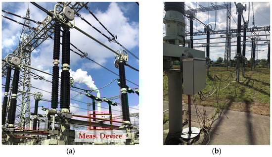
Figure 11.
Measurement system installed in the substation. (a) CDS on the base of a disconnector; (b) Control cabinet on the concrete base of a circuit breaker.
The value of the stray capacitance C1 depends on the distance and layout. Additionally, there is a coupling between the adjacent phases and the sensor, influencing its output voltage Vout, as illustrated in Figure 12.
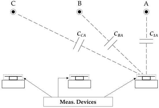
Figure 12.
Coupling capacitances between a CDS and adjacent phases.
Figure 12 shows only the coupling capacitances between the CDS installed in phase A and the three high-voltage connections. The same happens with the CDSs installed in phases B and C. To mitigate cross-coupling effects in the measurement, it is necessary to calibrate the measurement system. Two calibration techniques are examined:
- Simplified method (SM);
- Compensation of coupling capacitances (CCC).
4.1. Calibration Using the Simplified Method
The first calibration method compares the voltage values measured by the CDSs with the AC voltage from a substation divider at 50 Hz. In this case, the primary voltage measured by a capacitive voltage transformer serves as the reference. During the installation, the RMS value of the primary phase voltage was 238.45 kV, assuming a balanced three-phase system. The RMS voltages measured by the CDSs for phases A, B, and C were 2.03 V, 1.68 V, and 1.89 V, respectively. Therefore, the calculated voltage ratios for devices MD1, MD2, and MD3 are 117,461:1, 141,932:1, and 126,162:1, respectively. The voltage ratios can be set directly in the power quality monitor. Figure 13 shows the reference primary voltage (Vin) and the measured voltage (Vmeas) considering the calculated voltage ratio.
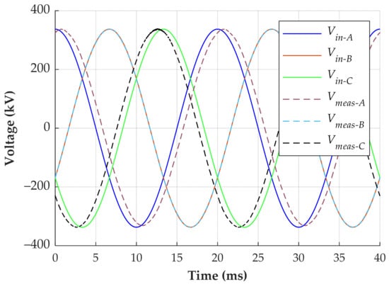
Figure 13.
Comparison between the reference and measured voltages.
In phase B, the reference and measured voltages are in phase. It happens due to the symmetrical influence of phases A and C on the device installed in phase B. However, the measured voltage of phase A is delayed by 14.14° with respect to the reference voltage of the same phase due to the influence of phases B and C. Similarly, the measured voltage of phase C leads the reference voltage by 13.12° due to the influence of phases A and B.
This calibration method is generally suitable for measuring steady-state voltages. It is straightforward to implement directly in the power quality monitor. However, the coupling between the measurement devices and adjacent phases may introduce notable errors when measuring electromagnetic transients, as will be shown in Section 5.
4.2. Compensation of the Coupling Capacitances
Given the constraints of the simplified method, especially in measuring transient overvoltages, a post-processing calibration method is developed. This method considers the coupling capacitances between the sensors and the high-voltage connections of the three phases to reconstruct the primary voltages from the measured output voltages.
This calibration method also requires the information of the steady-state primary voltage during the installation of the measurement system. The same primary voltage measured by a CVT and the corresponding output signals of the CDSs are used. The primary voltages are considered symmetrical, with the same amplitude and a phase difference of 120°. Therefore, the primary phase voltages are expressed in phasor notation as:
where Vp is the peak voltage measured by the CVT, in this case 337.22 kV.
Given the schematic diagram shown in Figure 12, an equivalent circuit for the measurement device installed in phase A is established to calculate the output voltage as a function of the primary voltage. The resulting equivalent circuit is presented in Figure 14.
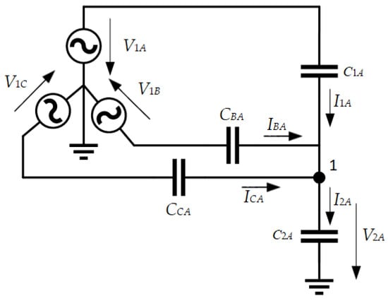
Figure 14.
Equivalent circuit representing the measurement device installed in phase A.
Applying Kirchhoff’s current law for node 1, the current I2A can be calculated as:
where
Substituting the equations from (5) into Equation (4), the output voltage V2A is calculated as:
The capacitance C2A has a value of approximately 50 nF, which is much higher than the stray capacitances C1A, CBA, and CCA, usually less than 1 pF. Therefore, Equation (6) can be simplified as:
The same concept and simplifications can be applied to the devices installed in phases B and C. Then, the output voltages are calculated as:
Equation (8) describes a linear system wherein the coefficient matrix depends on the stray capacitances and the user-defined capacitances C2. Since the stray capacitances have a unique value for a particular layout, there is only one physical solution for this system. However, all stray capacitances are unknown, leading to nine unknown parameters. The symmetry in the sensor installation reduces the number of unknown parameters, yet even in this scenario, the system may not be entirely determined.
Assuming identical influences of phases A and C on the sensor installed in phase B, CAB is equal to CCB, and V2B has the same phase as V1B in steady-state voltage calibration. Additionally, the influence of phase B on the sensors in phases A and C is assumed to be the same, resulting in CBA being equal to CBC. The summarized assumptions are as follows:
As previously stated, the linear system has mathematically infinite solutions, even with the assumptions outlined in (9). One potential approach, explored in other works [30,31,32], is to neglect the coupling capacitance between the outer phases, i.e., to consider CCA and CAC equal to 0. However, this choice may result in substantial errors when evaluating transient overvoltages. An alternative is to assign values obtained from FEM simulation to these parameters. Upon defining CCA, all parameters can be calculated by formulating the equations presented in (8), considering the assumptions given in (9).
The measurement system is calibrated using five distinct values of CCA, ranging from 0 to 0.2 pF, to assess the impact of coupling between the outer phases. The values have been chosen so that the calculated parameters are of the same order of magnitude as those obtained in the FEM simulation. The calculated parameters are shown in Table 2.
Table 2.
Set of stray capacitances calculated from different CCA values.
A transient overvoltage is reconstructed using the five parameter sets from Table 2. Figure 15 shows the signals from phase C, where the maximum overvoltage occurred.
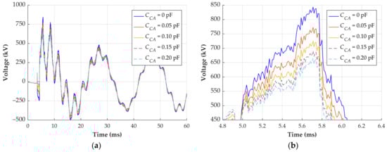
Figure 15.
Transient overvoltage reconstruction with different calibration parameters. (a) Response of phase C; (b) zoomed waveforms on the region of maximum overvoltage.
In the scenario where CCA is not considered (parameter set 1), the reconstructed signal exhibits a maximum overvoltage of 843 kV. Conversely, when CCA is 0.20 pF (parameter set 5), the reconstructed signal reaches only 665 kV. This difference of 178 kV represents 21.1%. Therefore, neglecting the coupling capacitance between the outer phases may lead to substantial errors in reconstructing the primary voltage. The question that arises is how to compute the correct coupling capacitances.
Based on the established principle of parallel plate capacitors, some configurations yield a capacitance inversely proportional to the distance between the electrodes. Hence, the initial investigation aimed to establish this correlation for the specific layout where the measurement system was installed. However, this relationship could not be established.
Then, an investigation is conducted to determine if the stray capacitances exhibit an inverse proportionality to the square of the distance, represented as follows:
where dAA, dBA, and dCA are the distances from the CDS installed in phase A to the high-voltage connections of phases A, B, and C, respectively.
Based on the information presented in (10) and considering that the permittivity and electrode area are identical for all phases, three normalized ratios can be calculated:
If the assumption that the capacitance is inversely proportional to the square of the distance is accurate, a set of stray capacitances satisfying the equations in (11) can be identified. Figure 16 shows the normalized ratios for different parameters, represented by the stray capacitance CCA.
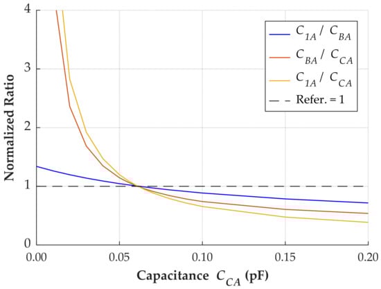
Figure 16.
Normalized ratios according to different values of stray capacitances.
When the capacitance CCA is 0.061 pF, the three normalized ratios become equal to 1. It indicates that a specific set of parameters satisfies the three equations given in (11). The parameters for the layout of this case study are presented in Table 3.
Table 3.
Set of stray capacitances calculated for the specific layout.
The correlation between the stray capacitances and the square of the distance has been demonstrated for the layout where the measurement system was installed. However, further investigation is necessary to confirm its validity for other configurations. If this correlation cannot be clearly established, alternative solutions include neglecting the coupling capacitance between the outer phases or estimating it using FEM simulations.
5. Measurement Results
The measurement system has been installed in the substation for one year, recording transients associated with transmission line switching and other disturbances. This section outlines the reconstruction of three transient signals using the calibration methods discussed in Section 4 and provides a statistical analysis of the recorded transients.
5.1. Comparison of Calibration Methods
As detailed in Section 4.1, the calibration provided by the simplified method is appropriate for measuring steady-state voltages. However, it may lead to significant errors when reconstructing transient signals. Therefore, the recommended approach is to utilize the method outlined in Section 4.2, which compensates for coupling capacitances. Nevertheless, calculating the coupling capacitances can be challenging, and a simplification can be made by considering the coupling capacitance between the outer phases as neglectable.
To assess the dissimilarities in the reconstruction of real transient signals, three transients are evaluated using the following methods and parameters:
- Simplified method (SM);
- Compensation of coupling capacitances (CCC) with CCA = 0 pF;
- Compensation of coupling capacitances (CCC) with CCA = 0.061 pF.
The first transient (also shown in Section 4) occurs due to the energization of the transmission line. Figure 17 shows the reconstructed signals for phase C (most critical).
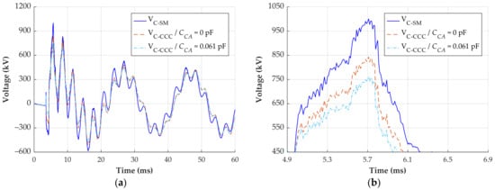
Figure 17.
Transient overvoltage reconstruction—line energization. (a) Response of phase C; (b) zoomed waveforms on the region of maximum overvoltage.
The signal reconstructed using the CCC method with a CCA of 0.061 pF is considered the reference. The maximum voltage of this signal is 761 kV. Ignoring the CCA in the CCC method results in a maximum voltage of 843 kV, representing a difference of 82 kV or 10.8%. The signal reconstructed with the simplified method has a maximum voltage of 1000 kV, indicating a difference of 31.4%.
The second signal is also a transient that occurs during the energization of the transmission line. The signal reconstruction of phase C, where the maximum negative overvoltage happened, is shown in Figure 18.
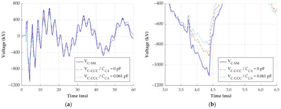
Figure 18.
Transient overvoltage reconstruction—line energization. (a) Response of phase C; (b) zoomed waveforms on the region of maximum negative overvoltage.
Considering again the signal reconstructed using the CCC method with a CCA of 0.061 pF as reference, the maximum negative voltage is −813 kV. Employing the CCC method with neglected CCA results in a maximum negative voltage of −916 kV, representing a difference of 103 kV or 12.7%. The signal reconstructed using the simplified method has a maximum negative voltage of −1107 kV, representing a difference of 294 kV or 36.2%. Therefore, the simplified method evidently overestimates the maximum overvoltage of the analyzed transients, whereas the difference ranging from 10% to 13% when ignoring CCA may or may not be considered acceptable, depending on the evaluation’s objective.
The third evaluated transient was recorded during the de-energization of the transmission line. The reconstructed signals are shown in Figure 19.
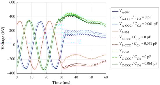
Figure 19.
Transient overvoltage reconstruction—line de-energization.
The most significant difference between the reconstructed signals is observed in phase B. The simplified method indicates a difference of up to 148 kV compared to the CCC method with a CCA of 0.061 pF. Moreover, the CCC method with neglected CCA and CCC method with a CCA of 0.061 pF have a maximum difference of approximately 30 kV. For this signal, no critical voltage level for equipment operation is identified. Consequently, the utilization of the simplified method would not compromise the evaluation.
5.2. Statistical Analysis of Transient Signals
During the one-year measurement campaign, the measurement system recorded 142 transient events. Table 4 shows the classification of these transients.
Table 4.
Number of transient events recorded by the measurement system.
Sixty-one percent of all recorded transients originate from external disturbances, such as circuit switching in the same substation or other perturbations in the power system. These signals are transients that return to the previous steady-state within a few milliseconds, meaning that there is no change in the state (closed/open) of the transmission line. The transmission line underwent 28 de-energizations and 27 energizations during the one-year period. This difference occurs because the line was energized when the measurement system was installed and de-energized when the system was removed.
The most critical transient overvoltages occurred during the energization of the transmission line. Therefore, a statistical analysis of the maximum voltage of the recorded transients is performed and the results are presented in Figure 20.
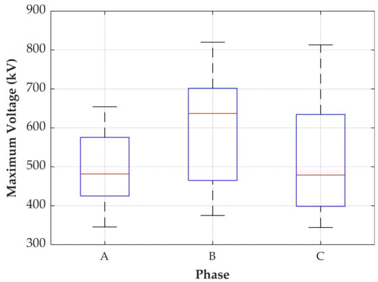
Figure 20.
Maximum voltage measured during the energization of the transmission line.
The median of the maximum voltage registered for phases A, B, and C are 482 kV, 637 kV, and 479 kV, respectively. The maximum overvoltages are 654 kV, 820 kV, and 813 kV, respectively. Therefore, the maximum registered overvoltage, measured in phase B, represents about 2.4 times the rated peak voltage. Figure 21 shows the transient signal with the highest maximum (negative) overvoltage.
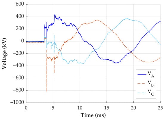
Figure 21.
Transient signal with the maximum measured overvoltage.
6. Conclusions
Accurately measuring and investigating electromagnetic transients is gaining importance with the increasing integration of renewable energy sources into the power grid. This paper introduces a measurement system based on capacitive electric field sensors capable of accurately measuring fast transients due to its broadband response. The measurement system was installed in a high-voltage substation for one year, recording 142 transient events. The installation process is straightforward and does not require de-energizing the bay.
Calibration is essential for measuring transient overvoltages using the proposed measurement system. This paper discusses two techniques: the simplified method and the CCC method. The simplified method can measure steady-state voltages, but it has been proven inaccurate for measuring transients. On the other hand, the CCC method, which accounts for the coupling capacitances between the measurement devices and the three phases, is the most appropriate for reconstructing transient overvoltages. All coupling capacitances were successfully calculated based on the layout and simplifications. However, neglecting the coupling capacitance between the external phases is acceptable if no relation between the layout (distances) and the calculated capacitances can be established. This study found that neglecting it resulted in a difference between 10% and 13%.
Finally, the study demonstrates that the proposed measurement system serves as an efficient and flexible solution for the long-term monitoring of transient overvoltages in a high-voltage substation, especially for fast transients requiring broadband measurement.
Author Contributions
Conceptualization, M.B. and S.T.; methodology, F.L.P. and S.T.; software, F.L.P.; validation, F.L.P. and S.T.; investigation, F.L.P.; resources, M.B. and S.T.; writing—original draft preparation, F.L.P.; writing—review and editing, M.B. and S.T.; visualization, F.L.P.; supervision, M.B. and S.T. All authors have read and agreed to the published version of the manuscript.
Funding
This research received no external funding.
Institutional Review Board Statement
Not applicable.
Informed Consent Statement
Not applicable.
Data Availability Statement
Data are contained within the article.
Acknowledgments
The authors gratefully acknowledge the support of TransnetBW GmbH. Special appreciation is expressed to Kai A. Alsdorf for his significant contributions.
Conflicts of Interest
The authors declare no conflicts of interest.
References
- CIGRE TB 577A; Electrical Transient Interaction between Transformers and the Power System—Part 1: Expertise. JWG A2/C4.39; CIGRE: Paris, France, 2014.
- CIGRE TB 577B; Electrical Transient Interaction between Transformers and the Power System—Part 2: Case Studies. JWG A2/C4.39; CIGRE: Paris, France, 2014.
- Probst, F.L.; da Luz, M.V.F.; Tenbohlen, S. Modeling of a capacitive voltage transformer for evaluation of transient response in conformity with the IEC 61869-5 Standard. Electr. Power Syst. Res. 2023, 223, 109591. [Google Scholar] [CrossRef]
- CIGRE TB 881; Electromagnetic Transient Simulation Models for Large-Scale System Impact Studies in Power Systems Having a High Penetration of Inverter-Connected Generation. WG C4.56; CIGRE: Paris, France, 2022.
- IEC 60071-1; Insulation Co-Ordination—Part 1: Definitions, Principles and Rules, Ed. 9.0. International Electrotechnical Commission: Geneva, Switzerland, 2019.
- IEC 60071-2; Insulation Co-Ordination—Part 2: Application Guidelines, Ed. 4.0. International Electrotechnical Commission: Geneva, Switzerland, 2018.
- Vermeulen, H.; Davel, P. Voltage harmonic distortion measurements using capacitive voltage transformers. In Proceedings of the IEEE AFRICON 1996, Stellenbosch, South Africa, 27 September 1996; Volume 2, pp. 1012–1017. [Google Scholar]
- Meyer, J.; Stiegler, R.; Klatt, M.; Elst, M.; Sperling, E. Accuracy of harmonic voltage measurements in the frequency range up to 5 kHz using conventional instrument transformers. In Proceedings of the 21st International Conference on Electricity Distribution (CIRED 2011), Frankfurt, Germany, 6–9 June 2011. [Google Scholar]
- Buchhagen, C.; Fischer, M.; Hofmann, L.; Däumling, H. Metrological determination of the frequency response of inductive voltage transformers up to 20 kHz. In Proceedings of the 2013 IEEE Power & Energy Society General Meeting, Vancouver, BC, Canada, 21–25 July 2013; pp. 1–5. [Google Scholar] [CrossRef]
- Tong, L.; Liu, Y.; Chen, Y.; Su, S.; Liang, P. A CVT based lightning impulse wave measuring method using convolutional neural network. In Proceedings of the 2021 IEEE 4th International Electrical and Energy Conference (CIEEC), Wuhan, China, 20–30 May 2021; pp. 1–6. [Google Scholar]
- Zare, M.; Mirzaei, A.; Askarian Abyaneh, H. Designing a compensating electronic circuit to enhance capacitive voltage transformer characteristics. In Proceedings of the 9th Power Systems Protection and Control Conference (PSPC2015), Tehran, Iran, 11–14 October 2015; pp. 12–18. [Google Scholar]
- Kang, Y.C.; Zheng, T.Y.; Choi, S.W.; Kim, Y.H.; Kim, Y.G.; Jang, S.I.; Kang, S.H. Design and evaluation of a compensating algorithm for the secondary voltage of a coupling capacitor voltage transformer in the time domain. IET Gener. Transm. Distrib. 2009, 3, 793–800. [Google Scholar] [CrossRef]
- Zadeh, H.; Zuyi, L. A compensation scheme for CVT transient effects using artificial neural network. Electr. Power Syst. Res. 2008, 78, 30–38. [Google Scholar] [CrossRef]
- De La Hoz, M.; Chacón, J.; Sørensen, D.A.; Larrinaga, U.Z.; Barón, C.R. Harmonic measurements in a capacitive voltage transformer: Improvement considering the transformer’s design parameters. In Proceedings of the 2021 International Conference on Smart Energy Systems and Technologies (SEST), Vaasa, Finland, 6–8 December 2021; pp. 1–6. [Google Scholar]
- Ghassemi, F.; Gale, P.; Cumming, T.; Coutts, C. Harmonic voltage measurements using CVTs. In Proceedings of the 2004 IEEE Power Engineering Society General Meeting, Denver, CO, USA, 6–10 June 2004; Volume 1, p. 482. [Google Scholar]
- Fu, C.Z.; Si, W.R.; Zhao, D.D.; Huang, H.; Jin, H.; Zhao, W.B. Research on the method for transient overvoltage measurement using CVT within a capacitor C3. In Proceedings of the 2016 International Conference on Condition Monitoring and Diagnosis (CMD), Xi’an, China, 25–28 September 2016; pp. 1028–1030. [Google Scholar]
- Stirl, T. Online monitoring of capacitance-graded bushing on power transformers. In Proceedings of the ETG Technical Seminar No. 97, Cologne, Germany, 9–10 March 2004; pp. 115–120. (In German). [Google Scholar]
- Stirl, T.; Skrzypek, R.; Tenbohlen, S.; Vilaithong, R. On-line condition monitoring and diagnosis for power transformers their bushings, tap changer and insulation system. In Proceedings of the 2006 International Conference on Condition Monitoring and Diagnosis (CMD), Changwon, Republic of Korea, 2–5 April 2006. [Google Scholar]
- Ma, G.M.; Li, C.R.; Quan, J.T.; Jiang, J. Measurement of VFTO based on the transformer bushing sensor. IEEE Trans. Power Deliv. 2011, 26, 684–692. [Google Scholar] [CrossRef]
- Tenbohlen, S.; Kattmann, C.; Brugger, T. Power quality monitoring in power grids focusing on accuracy of high frequency harmonics. In Proceedings of the 2018 Cigré Session, Paris, France, 26–31 August 2018. [Google Scholar]
- Kattmann, C.; Siegel, M.; Tenbohlen, S.; Bruger, T. Power quality measurement in high voltage grids using transformer bushings. In Proceedings of the VDE Hochspannungstechnik, Berlin, Germany, 12–14 October 2018. (In German). [Google Scholar]
- Botha, M. Wideband Modelling of Capacitive Voltage Sensors for Open-Air Transmission Line Applications. Ph.D. Thesis, Electrical Engineering, University of Stellenbosch, Stellenbosch, South Africa, 2002. [Google Scholar]
- Liu, H.; Ma, G.; Qin, W.; Wang, W.; Du, H.; Wang, L.; Zhai, S.; Zeng, F.; Han, W. A low-cost and high-performance self-trigger method for high-voltage transient measurement. High Volt. 2022, 8, 412–420. [Google Scholar] [CrossRef]
- Han, R.; Yang, Q.; Sima, W.; Zhang, Y.; Sun, S.; Liu, T.; Chen, S. Non-contact measurement of lightning and switching transient overvoltage based on capacitive coupling and pockels effects. Electr. Power Syst. Res. 2016, 139, 93–100. [Google Scholar] [CrossRef]
- Sun, S.; Ma, F.; Yang, Q.; Ni, H.; Bai, T.; Ke, K.; Qiu, Z. Research on non-contact voltage measurement method based on near-end electric field inversion. Energies 2023, 16, 6468. [Google Scholar] [CrossRef]
- Xiao, D.; Xie, Y.; Ma, Q.; Zheng, Q.; Zhang, Z. Non-contact voltage measurement of three-phase overhead transmission line based on electric field inverse calculation. IET Gener. Transm. Distrib. 2018, 12, 2952–2957. [Google Scholar] [CrossRef]
- Chen, K.-L.; Guo, Y.; Ma, X. Contactless voltage sensor for overhead transmission lines. IET Gener. Transm. Distrib. 2018, 12, 957–966. [Google Scholar] [CrossRef]
- Si, D.; Wang, J.; Wei, G.; Yan, X. Method and experimental study of voltage measurement based on electric field integral with Gauss–Legendre algorithm. IEEE Trans. Instrum. Meas. 2020, 69, 2771–2778. [Google Scholar] [CrossRef]
- Wang, J.; Ban, S.; Yang, Y. A differential self-integration D-dot voltage sensor and experimental research. IEEE Sens. J. 2015, 15, 3846–3852. [Google Scholar] [CrossRef]
- Wouters, P.A.A.F.; Barakou, F.; Gargari, S.M.; Smit, J.; Steennis, E.F. Accuracy of switching transients measurement with open-air capacitive sensors near overhead lines. In Proceedings of the 2018 IEEE International Conference on High Voltage Engineering and Application (ICHVE), Athens, Greece, 10–13 September 2018; pp. 1–4. [Google Scholar] [CrossRef]
- Barakou, F.; Wouters, P.A.A.F.; Gargari, S.M.; Smit, J.; Steennis, E.F. Merits and challenges of a differentiating-integrating measurement methodology with air capacitors for high-frequency transients. In Proceedings of the 2018 Cigré Session, Paris, France, 26–31 August 2018. [Google Scholar]
- Barakou, F.; Steennis, F.; Wouters, P. Accuracy and reliability of switching transients measurement with open-air capacitive sensors. Energies 2019, 12, 1405. [Google Scholar] [CrossRef]
- Brügger, T.H. Transient and harmonic measurements with unconventional instrument transformers. In Proceedings of the Stuttgarter Hochspannungssymposium, Stuttgart, Germany, 21–22 June 2022. (In German). [Google Scholar]
- Probst, F.L.; Beltle, M.; Gerber, M.; Tenbohlen, S.; Alsdorf, K.A. Measurement of switching transient overvoltages with a capacitive electric field sensor. Electr. Power Syst. Res. 2023, 223, 109619. [Google Scholar] [CrossRef]
- Probst, F.L.; Beltle, M.; Gerber, M.; Tenbohlen, S.; Alsdorf, K.A. Using capacitive electric field sensors to measure transient overvoltages: A case study. In Proceedings of the International Symposium on High Voltage Engineering (ISH), Glasgow, Scotland, 28 August–1 September 2023. [Google Scholar]
- CST Studio Suite [Computer Software]. 2021. Available online: http://www.cst.com (accessed on 23 November 2023).
- Linear Technology. Fast Settling, JFET Input Operational Amplifier. LT1122 Datasheet, Revision B February 2014. Available online: https://www.analog.com/media/en/technical-documentation/data-sheets/1122fb.pdf (accessed on 19 February 2024).
- Traco Power. DC/DC Converter TVN 5WI Series, 5 Watt. TVN 5-4825WI Datasheet, Revision September 2023. Available online: https://www.tracopower.com/de/deu/tvn5wi-datasheet (accessed on 19 February 2024).
- BSS Hochspannungstechnik. PQM-800 Power Quality Monitor. PQM-800 Datasheet. Available online: https://www.bss-hochspannungstechnik.de/pdf/Datasheet%20PQM-800.pdf (accessed on 23 November 2023).
- IEC 60060-1; High-Voltage Test Techniques—Part 1: General Definitions and Test Requirements. International Electrotechnical Commission: Geneva, Switzerland, 2010.
- Rohde & Schwarz. Vector Network Analyzer Family ZVR. VNA ZVRE Datasheet. Available online: https://www.testequipmenthq.com/datasheets/Rohde-Schwarz-ZVRE-Datasheet.pdf (accessed on 19 February 2024).
Disclaimer/Publisher’s Note: The statements, opinions and data contained in all publications are solely those of the individual author(s) and contributor(s) and not of MDPI and/or the editor(s). MDPI and/or the editor(s) disclaim responsibility for any injury to people or property resulting from any ideas, methods, instructions or products referred to in the content. |
© 2024 by the authors. Licensee MDPI, Basel, Switzerland. This article is an open access article distributed under the terms and conditions of the Creative Commons Attribution (CC BY) license (https://creativecommons.org/licenses/by/4.0/).