
Design and Enhancement of a Fog-Enabled Air Quality Monitoring and Prediction System: An Optimized Lightweight Deep Learning Model for a Smart Fog Environmental Gateway


Abstract
1. Introduction
- Proposed a novel Fog-enabled Air Quality Monitoring and Prediction (FAQMP) system leveraging IoT with Fog Computing, LPWAN, and DL, aiming to support real-time and low-cost monitoring with accurate forecasting for decision support in smart cities.
- Developed a Smart Fog Environmental Gateway (SFEG) that introduces efficient Fog Intelligence in the FC layer through fog–cloud collaboration.
- Developed a user-friendly web application, namely EnviroWeb, to present real-time air quality AQI trends, forecasts, early warnings, and alerts to the users.
- Proposed a DL-based Seq2Seq GRU Attention model for multivariate multi-step time series air quality forecasting. The model demonstrates superior performance and stability in forecasting air quality for multiple time steps in comparison against baseline models.
- Developed an optimized lightweight DL model that facilitates efficient Fog Intelligence on the SFEG by striking a balance between computational efficiency and model performance.
2. Related Works
2.1. Air Quality Monitoring (AQM) Systems
2.2. Air Quality Forecasting Systems
2.3. Technical Enablers for Fog Intelligence in IoT Environmenst: Model Compression Techniques and Hardware Exploration
2.3.1. Model Compression
2.3.2. Exploring Hardware for Fog Intelligence
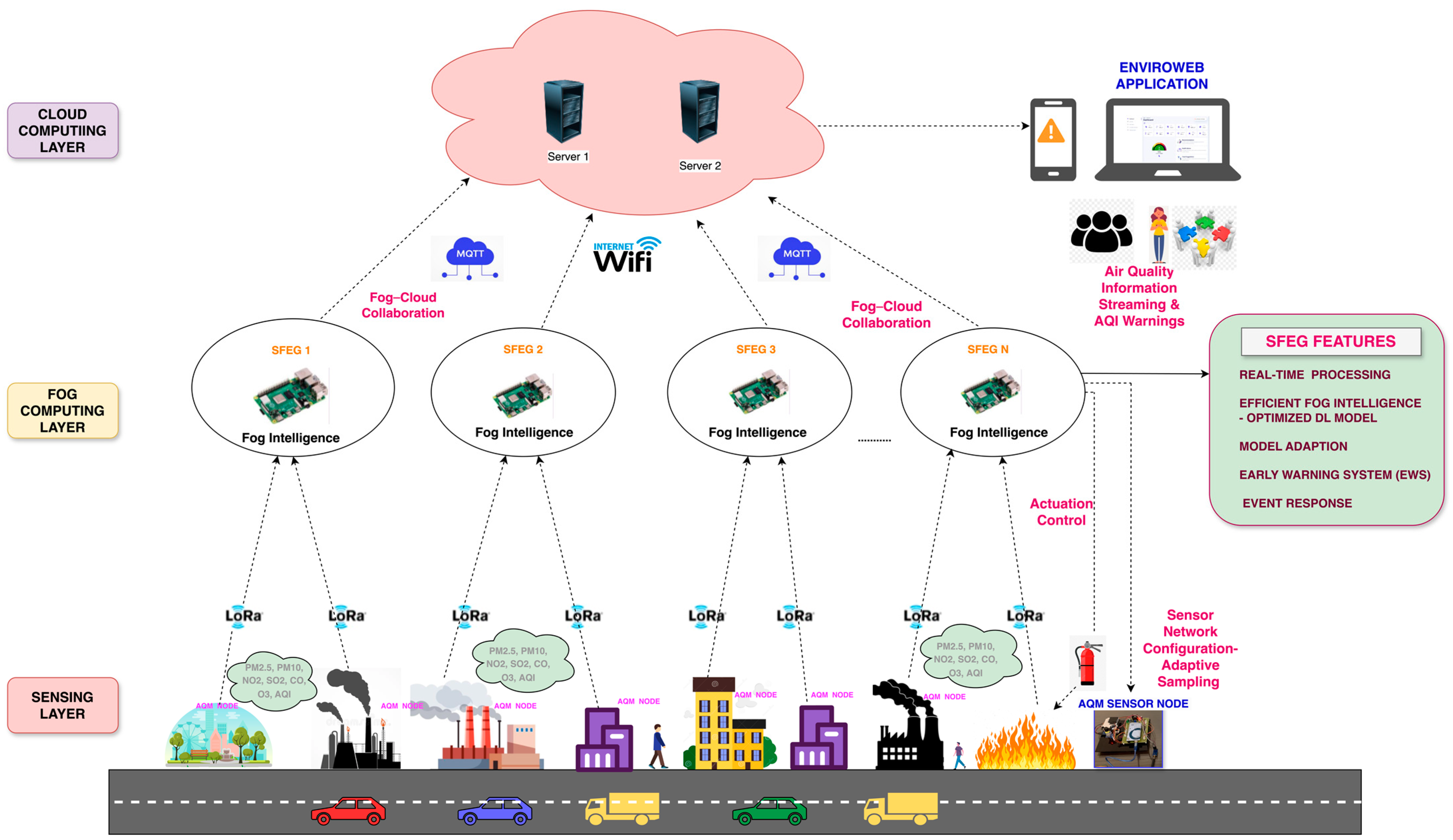
3. Proposed Approach: A Fog-Based IoT Architecture and Fog–Cloud Collaboration in the FAQMP System
3.1. Architecture of the FAQMP System and Hardware Implementation
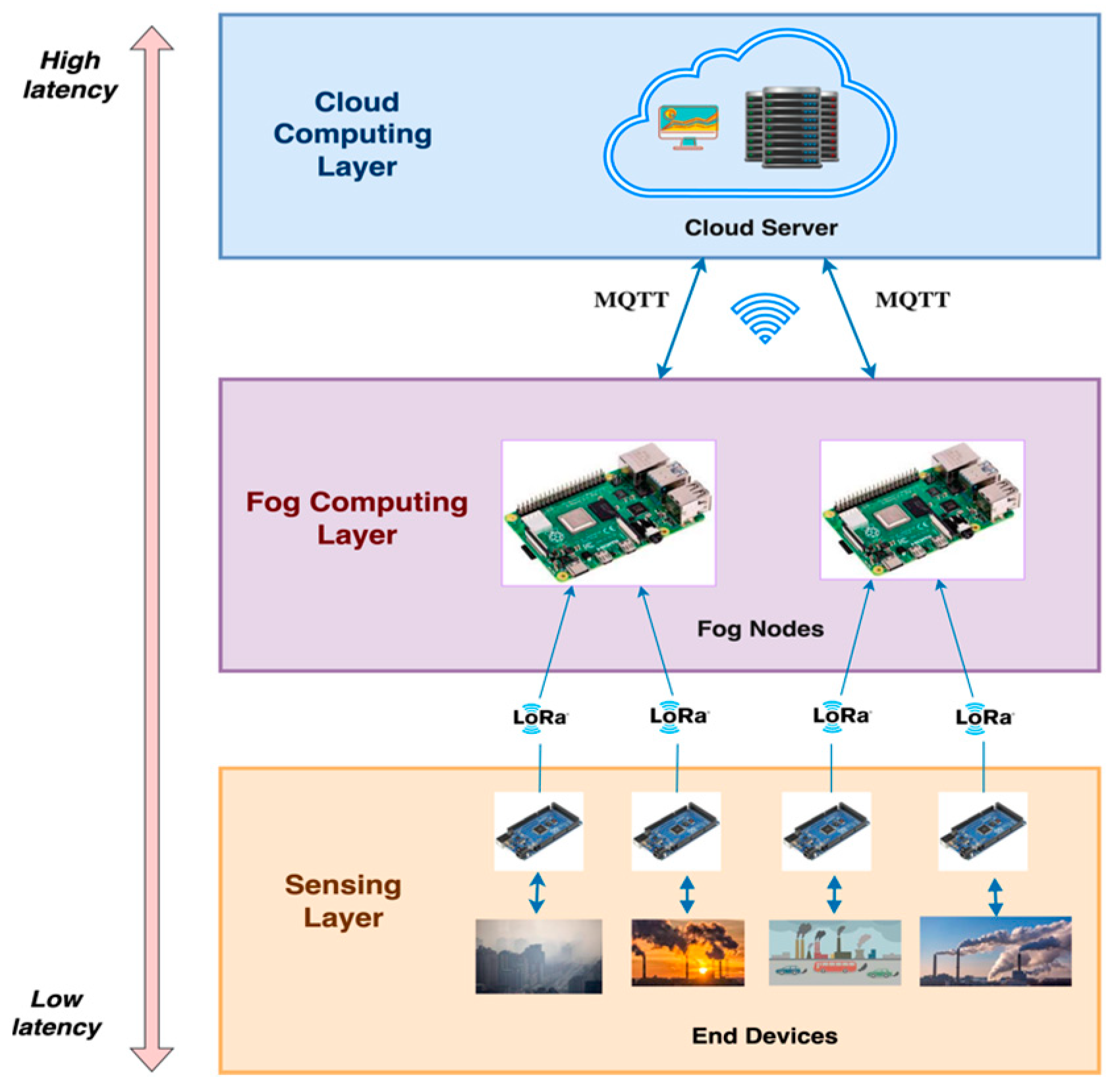
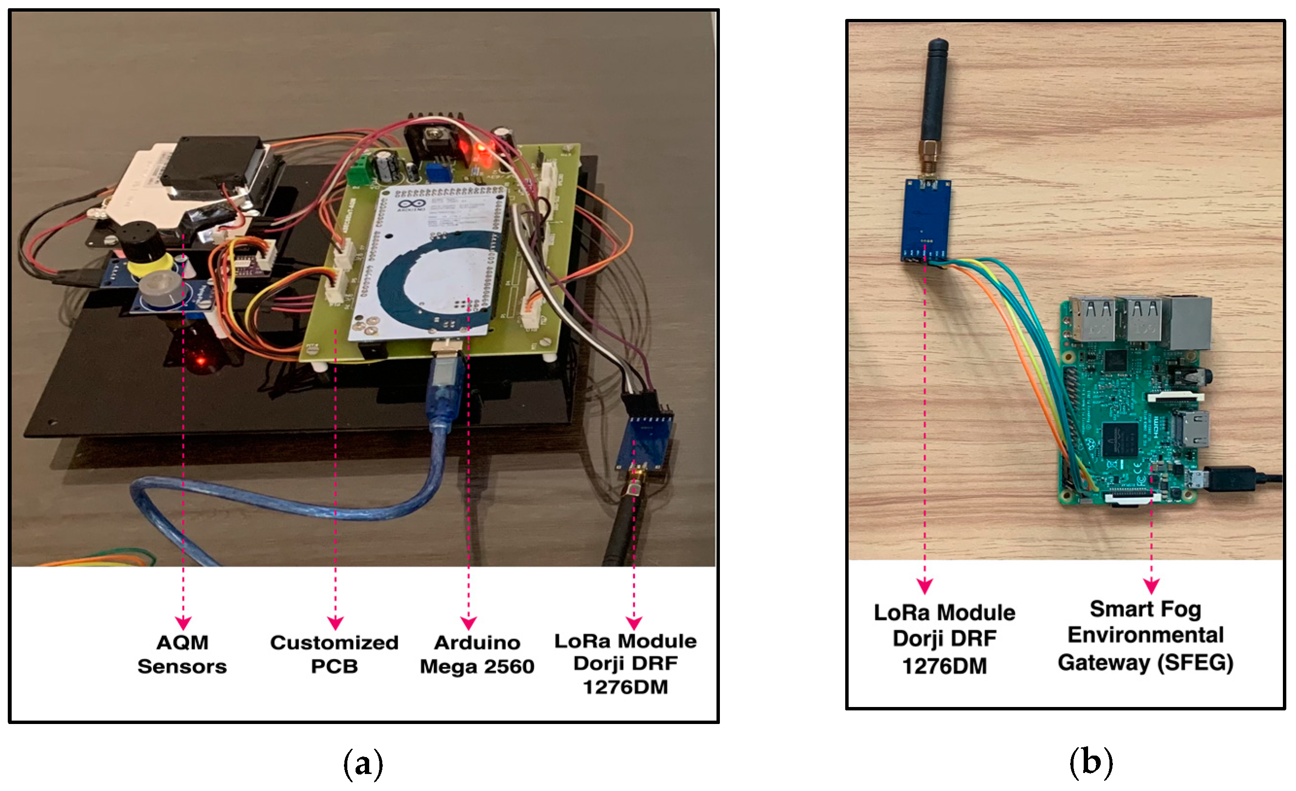
- Sensing layer: The sensing layer serves as the foundation for monitoring air quality levels. The primary component of this layer is the AQM sensor node, designed with a PCB configured to function as an end device, as shown in Figure 3a. The PCB modularly integrates an array of dedicated low-cost sensors that acquire pollutant and meteorological parameters, along with a LoRa communication module connected to the controller unit. The controller unit is an Arduino Mega 2560, which is a low-cost, low-power, and resource-constrained microcontroller. Moreover, low-cost sensors have gained importance in facilitating dense deployments, greater coverage, and portability over traditional static monitoring systems. The sensors, as discussed in Table 4, are selected based on their cost, precision, accuracy, range, ability to monitor gases, lifetime, and compatibility with the controller. In particular, the sensors, including SDS011, MICS4514, MQ131, MQ136, BME280, pyranometer, and MPXV7002DP, measure the values of PM2.5, PM10, NO2, SO2, CO, O3, temperature, pressure, humidity, SR, WS, and WD. Moreover, due to variations between sensors in production, it is recommended to calibrate before deployment [27,31] to ensure accuracy in the measured values. Thus, the sensors in our AQM system are calibrated before data acquisition. For instance, Algorithm 1 presents the steps to pre-calibrate sensors like MQ136, where the coefficients x and y are extrapolated based on the characteristic curve presented in the datasheet [88]. The pre-calibration ensures that the sensor provides accurate and reliable readings of the measured gas.
| Algorithm 1: Pre-Calibration of the MQ136 |
| calculation —Sensor resistance in the pure air); calculation —Sensor resistance in the presence of a specific gas); 3: Analog read sensor pin; 4: Collect various samples and determine the aggregate (S); S/clean air factor; 6: Extrapolate coefficients x and y from datasheet; 7: Estimate ppm values, ppm |
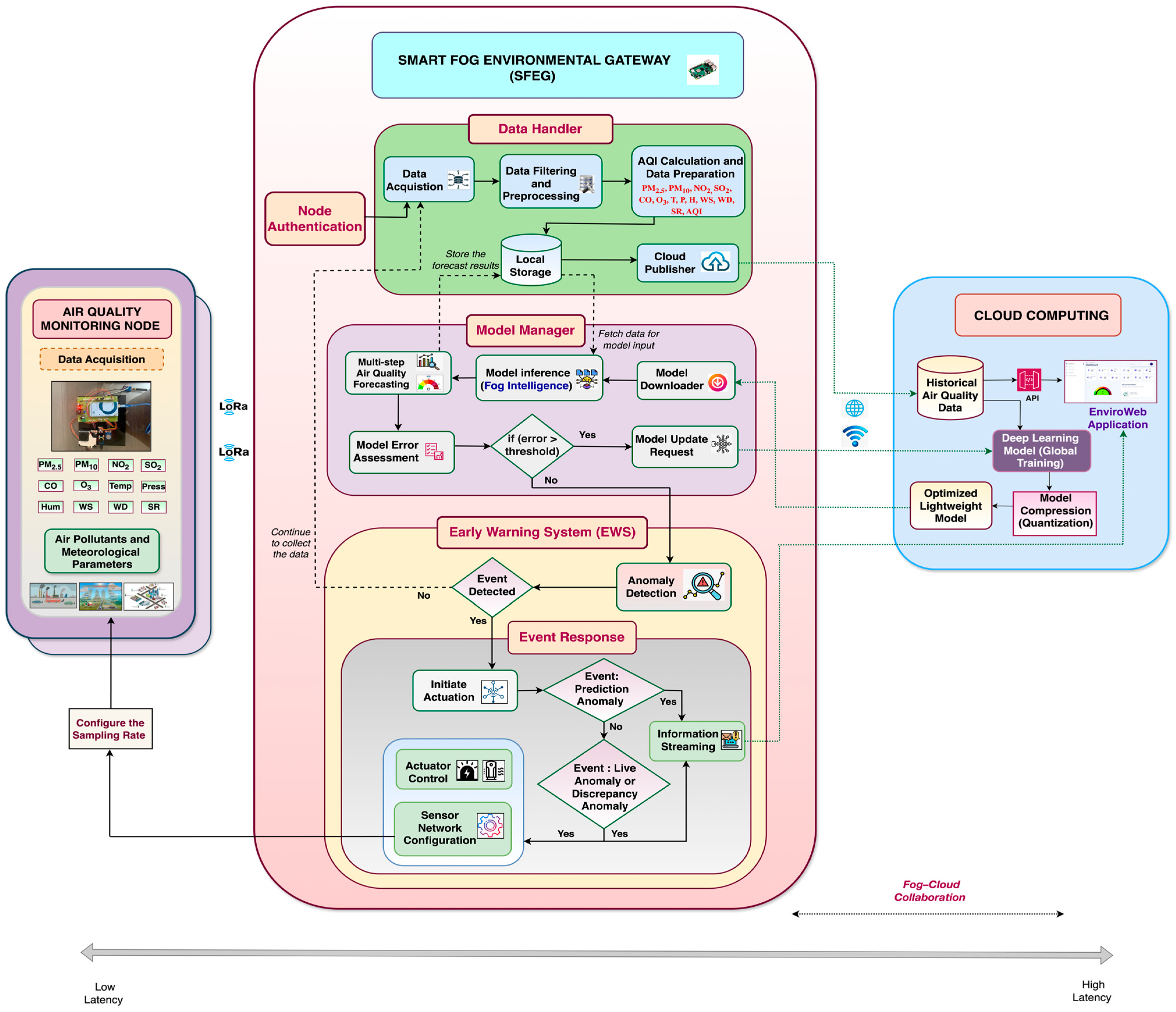
- Fog Computing (FC) Layer: FC is vital for air quality monitoring and forecasting due to its ability to offer computation and storage closer to the data sources with the benefits of minimized response time, optimized bandwidth efficiency, reliability, and reduced burden on the cloud. FC addresses the challenges of data processing, analysis, and transmission in dynamic environmental conditions. For the proof of concept, the proposed system utilizes a cost-effective Raspberry Pi 3 Model B+ as the fog gateway or fog node, as shown in Figure 3b. The fog gateway receives air quality sensor data from the sensing layer using LoRa module Dorji DRF1276DM. The received data are filtered and processed for further analysis. Fog intelligence is introduced by deploying an optimized DL model for on-device inference, enabling efficient processing by eliminating the need to constantly communicate with the cloud for processing. Moreover, the Early Warning System (EWS) detects anomalies and initiates an event response upon detecting dangerous AQI levels. Moreover, the real-time services offered by RPi for air quality data storage, management, communication, data analysis, early warnings, fog intelligence, and fog–cloud collaboration enable it to be a Smart Fog Environmental Gateway (SFEG). The services of the SFEG to manage the data and resources are detailed in Section 3.2. Furthermore, the forecast results and the air quality data are sent to the cloud using MQTT for historical storage and analysis.
- Cloud Computing (CC) Layer: The cloud layer at the top of the hierarchy centralizes and manages the data obtained from the SFEG in the FC layer. It offers a robust infrastructure to store and process historical air quality data, manage fog nodes, train complex DL models, and serve end-user applications. We chose the AWS platform as it offers a comprehensive suite of secure services like AWS IoT Core, AWS Lambda, DynamoDB, S3, CloudWatch, and Sage Maker, making it an ideal choice for our system requirements. Furthermore, a web application, namely EnviroWeb, is designed to present stakeholders with real-time air quality data, pollutant trends, AQI levels, forecasts, and early warnings using the data stored in the cloud.
3.2. Implementation of Fog–Cloud Collaboration in the Proposed FAQMP System
- Node Authentication: The SFEG’s node authentication module authenticates the AQM sensor nodes to join the SFEG network for continuous transmission of air quality data. Initially, this module sends an authentication number to the AQM node in the sensing layer via LoRa downlink. The AQM node integrates the received authentication number with the collected air quality, forming a payload for LoRa uplinking to the SFEG. Daemons on the SFEG listen for incoming messages, extract live data, including the authentication number, and verify them. If the number matches, the AQM sensor node is authenticated and can send data, ensuring secure and reliable transmission.
- Data Handler: The SFEG’s data handler filters and preprocesses the received air quality data. Missing values are imputed using linear interpolation, and the AQI is calculated and appended to the preprocessed data. Preprocessing tasks like data cleaning, filtering, aggregation, and formatting enhance the data before analysis. The final prepared data, including PM2.5, PM10, NO2, SO2, CO, O3, temperature, pressure, humidity, WS, WD, and SR, along with the AQI, are stored in the SFEG database to ensure seamless data recovery. SFEG data storage allows the system to remain stable and provide backup even during network outages and intermittent connectivity.
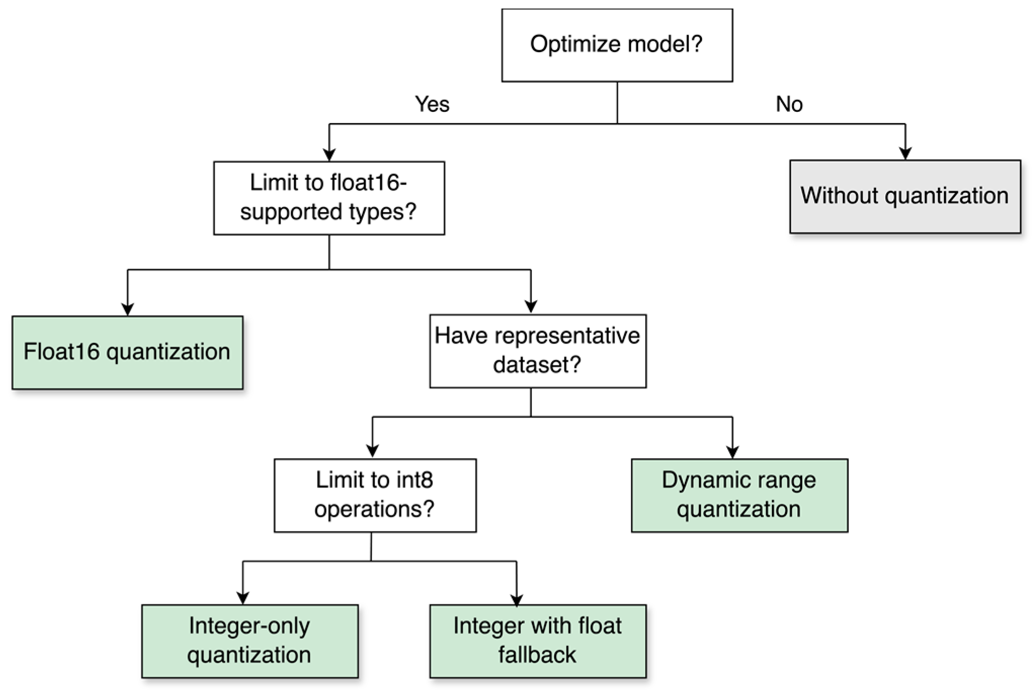
- Cloud Model Orchestrator: The cloud model orchestrator manages the training, optimization, and storage of the DL model in the cloud for deployment on the SFEG. At first, AWS Sage Maker facilitates model training with historical air quality data by leveraging the powerful compute instances. Based on the comparative analysis of various DL models presented, the Seq2seq GRU Attention model has good multi-step forecasting performance as analyzed from the results in Section 5.1.6. To make the model lightweight and efficient for SFEG, dynamic range quantization based on PTQ in model compression is applied, reducing its size and execution time while maintaining model accuracy. This optimized lightweight Seq2seq GRU Attention model, chosen based on the experimental results from Section 5.2, is then stored in AWS S3.
- Model Manager: By embracing fog–cloud collaboration, the model manager on the SFEG uses the model downloader to download the model from the AWS S3 bucket using the boto3 library. This model is deployed on the SFEG for inference, introducing efficient Fog Intelligence. Figure 5 illustrates the deployment pipeline [90] for the optimized DL model on a low-resource fog device like SFEG. The local air quality data are fetched, normalized, and fed into the model to generate multi-step forecasts for the next 3 h (12 time steps) at 15 min intervals in real time, without network delays. These live and meaningful forecasts are presented through the EnviroWeb application dashboard to the stakeholders.
- Early Warning System (EWS) Handler: The EWS Handler analyzes the live data and forecasted data to detect anomalies and provide insights into the potential issues with the air quality data, including seasonal deviations. If any anomaly exists in the live data based on the AQI threshold defined, it is referred to as a live data anomaly. On the other hand, if an anomaly exists in the forecasted values, it is referred to as a prediction anomaly. Similarly, if an anomaly exists in both live and forecasted data, it is referred to as a discrepancy anomaly. While processing, if an anomaly is detected, the event variable is updated with the anomaly type (e.g., live data anomaly), and then the sub-module of EWS, namely the event response module, is activated as presented in Figure 4.
- Event Response: Based on the nature of the event, the SFEG’s event response module makes timely decisions and initiates appropriate actions to address the anomaly. These actions include information streaming, actuator control, and sensor network configuration.
- (a)
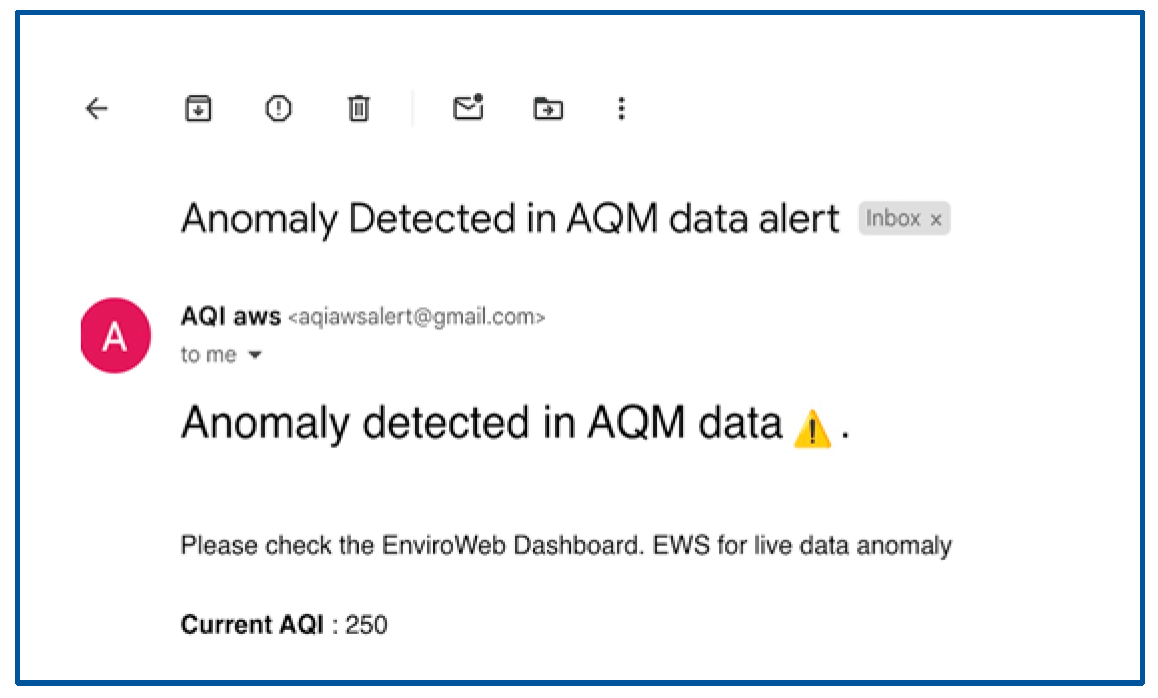
- Information Streaming: Timely alerts or notifications are sent to users via channels such as email, SMS, and EnviroWeb dashboards. This is crucial for providing immediate information about any detected anomalies, particularly those related to dangerous air quality levels. For testing purposes, we simulated a fire event where the AQI levels increased in the live data. This simulated spike activated the event response module, triggering an immediate reaction. As a result, an email alert was generated and received, as shown in Figure 6, demonstrating how the system works in real time to notify stakeholders about hazardous air quality conditions.
- (b)
- Sensor Network Configuration: During a live data anomaly, commands are sent to the controller of the AQM sensor node via LoRa downlinking. These commands adjust the AQM sensor node’s sampling rate to capture more detailed event information.
- (c)
- Actuator Control: During a live data anomaly, commands are sent to activate alarms, adjust ventilation systems, activate air purifiers, and control pollutant emission sources to maintain a healthy environment. This is crucial during time-critical hazardous events, such as dangerous air quality levels, fires, and gas leakages, to enable timely response by promptly reducing the severity of dangerous situations.
- Fog manager: The fog manager is mainly responsible for managing all the modules of the SFEG. It includes tasks such as resource allocation, data processing, data transmission, communication management, and overall coordination of activities within the FC environment.
3.3. EnviroWeb Application
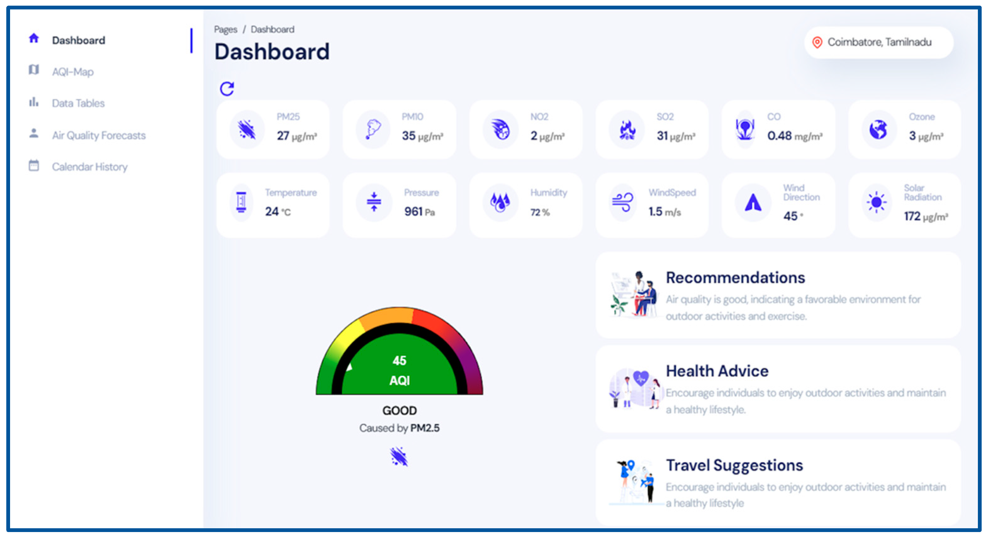
- Real-time Air Quality Data: The application offers real-time measurements of air pollution and meteorological data, as well as the Air Quality Index (AQI), as shown in Figure 7.
- Historical Data Analysis and Visualization: The application features customizable visualizations in charts and graphs to illustrate the historical pollution and AQI trends over a user-specified period (day, week, or month).
- Air Quality Forecast and Recommendations: The application presents AQI predictions for the next 3 h at an interval of 15 min. Based on the live and forecasted air quality data, decisions are made and recommendations are presented to the users related to health, travel, lifestyle changes, behavioral adjustments, and actions to reduce pollution levels.
- Smart Alerts: When an anomalous event or hotspot is detected based on the live and forecasted air quality levels, alerts are presented in the dashboard as a part of the EWS Handler’s actuation (information streaming), as discussed previously in Section 3.2.
- Maps: The interactive map uses color-coded markers based on the AQI level of a specific location, allowing the users to navigate and explore the surrounding AQM station locations and determine AQI hotspots.
- Data Export and Sharing: The data export and sharing feature allows users to export the monitoring and forecast data.
3.4. City-Wide Air Quality Management with FAQMP: Achieving Scalability and Real-Time Insights
3.4.1. Challenges and Bottlenecks in Scaling the Proposed FAQMP System
- Data Volume and Management: Increased data from a growing number of sensors nodes will demand robust processing and storage solutions at fog nodes, such as the SFEGs.
- Resource Management: As the number of AQM sensor node increases, managing computational resources efficiently becomes crucial, requiring careful resource allocation.
- Communication Efficiency: Deployment of thousands of sensors leads to higher network traffic. Therefore, ensuring efficient communication among the sensor node, SFEG, and the cloud layer is essential for seamless data exchange and low-latency processing.
- Resource Constraints: Fog nodes like SFEG typically have limited CPU, memory, and storage resources compared to cloud servers, a fact which constrains their ability to process large volumes of sensor data and run complex algorithms.
- Real-time Processing: Handling high volumes of air quality data and complex forecasting models while maintaining minimal latency and timely responses is challenging.
- Model adaption and Performance: DL models must adapt to varying air quality patterns and environmental conditions by continuous retraining, which can be resource-intensive.
- Maintenance and Management: Managing and calibrating numerous sensors to ensure accurate air quality data are complex tasks.
- Cost Management: Scaling involves higher costs for hardware, installation, maintenance, and ongoing operations.
- Data Security: Ensuring the security and privacy of sensitive information is crucial.
3.4.2. City-Wide Implementation of the FAQMP System—Addressing the Scalability Challenges
3.4.3. The Role of the FAQMP System in Shaping Public Health Policies and Urban Development
- Public Health Protection: The system provides real-time AQI monitoring and forecasts via EnviroWeb, offering health advisories to vulnerable populations to reduce pollutant exposure. The recommendations will allow citizens to make informed decisions about outdoor activities and travel for an enhanced quality of life.
- Timely Warnings and Responses: The EWS module of the FAQMP system detects anomalous pollution events and triggers alerts via email and EnviroWeb and captures detailed information through adaptive sensor sampling. Identifying pollution sources enables targeted interventions and regulations to decrease emissions.
- Proactive Measures: Multi-step forecasting helps predict future hour’s air quality trends, allowing urban planners to implement preemptive strategies in real time and manage pollution peaks.
- Dynamic Policy Adaptation: The FAQMP system enables the formulation and adjustment of policies related to environmental regulations, emission standards, industrial regulations, and urban design based on the real-time AQI data.
- Enhanced Urban Planning and Resource Allocation: The FAQMP system will help urban planners identify pollution hotspots based on AQI levels, enabling optimized resource allocation for pollution control and urban infrastructure improvements, such as green spaces and buffer zones.
- Traffic Management: The data from the FAQMP system will support optimizing traffic flow and congestion management strategies, leading to reduced vehicular emissions.
- Community Engagement and Sustainable Development: The system promotes transparency and public awareness through EnviroWeb, fostering community involvement and sustainable development.
- Economic Benefits: The FAQMP system reduces healthcare costs and environmental damage through efficient monitoring and targeted interventions.
4. Methodology
4.1. Gated Recurrent Unit (GRU)
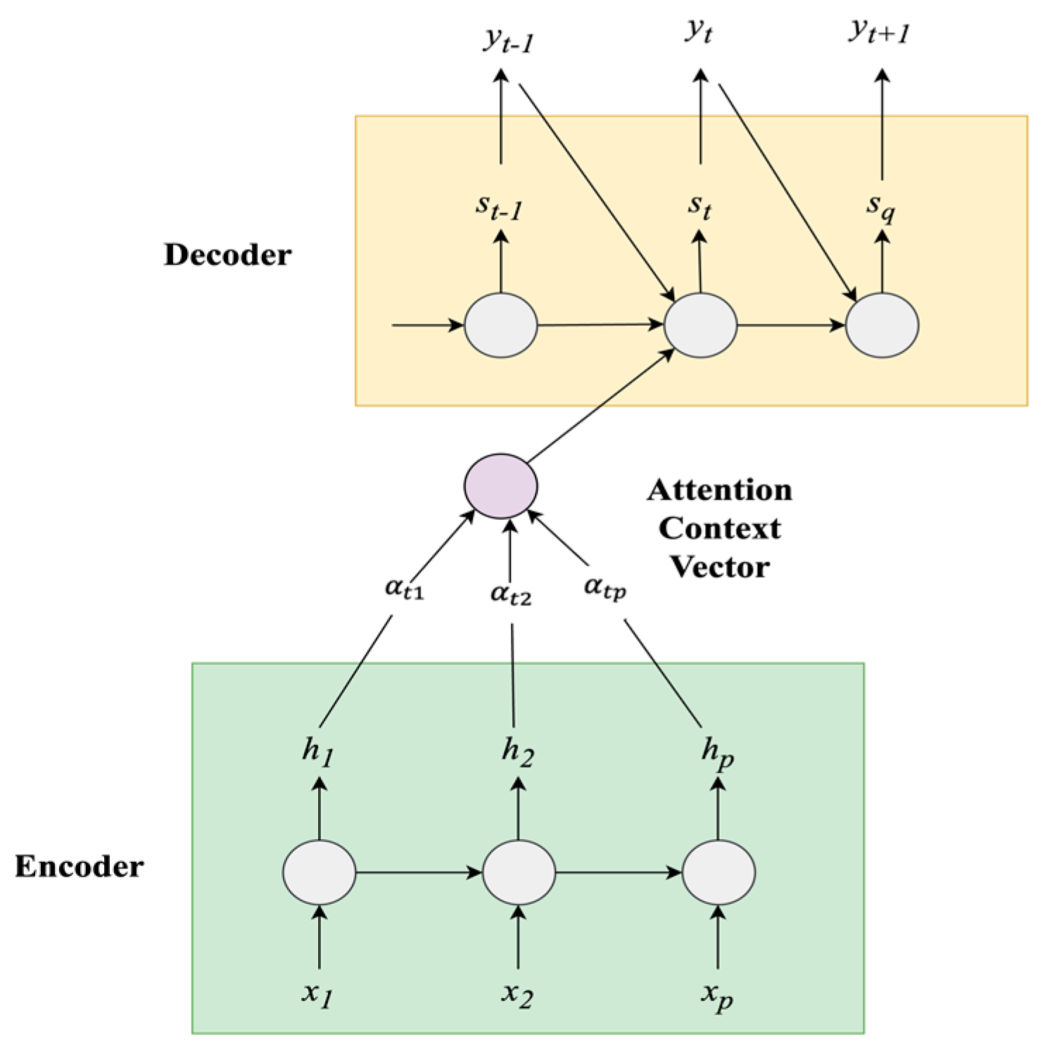
4.2. Sequence-to-Sequence (Seq2Seq) GRU Attention Model
- Encoder: The encoder is a GRU that processes the given input sequence to generate a sequence of hidden states [, where T is the length of the input sequence. At each encoding time step t, the hidden state is updated by using both the input vector and the previous hidden state , as illustrated in Equation (7).
- Attention Mechanism: The attention mechanism in the Seq2seq GRU-based Attention model allows focus on significant parts of the input sequence while generating output in the decoder, guided by attention scores.
- Attention Score Calculation: The “attention score” or “alignment score” for each encoder hidden state hi is calculated using a scoring function. The attention score et,i indicates how much importance the decoder’s previous state places on the specific encoder state hi. The attention score is calculated as illustrated in Equation (8).
- Attention weight calculation: Attention weights are the normalized version of the attention scores. After computing the attention scores , a softmax function is applied to these scores to obtain the temporal attention weights as displayed in Equation (9).where T denotes the length of the input sequence.
- Context vector calculation: The context vector is a fixed-size representation of the input sequence, calculated by combining the encoder’s hidden states with the attention weights as illustrated in Equation (10):
- 3.
- Decoder: The decoder is another GRU that reads the information from the context vector and its internal states to generate the output sequence. The context vector obtained from the attention mechanism is combined with the decoder’s previous hidden state and previous target output , then fed to the GRU unit to compute the current hidden state as in Equation (11). acts as an initial point to compute the output sequence.
- The output layer is a regression function that outputs the predicted value . The decoder generates the output sequence at each time step t based on the current hidden state , previous output , and context vector as expressed in Equation (12).
- W is the weight matrix; b is a bias vector, and represents the concatenation of the context vector, the current hidden state, and the previous output.
5. Experimental Evaluation
5.1. Experiment I: DL-Based Multivariate Multi-Step Forecasting
5.1.1. Dataset Description
5.1.2. Data Preprocessing
5.1.3. Experimental Settings and Baselines
5.1.4. Evaluation Metrics
5.1.5. Hyperparameter Tuning
5.1.6. Experimental Results: Analysis and Discussion
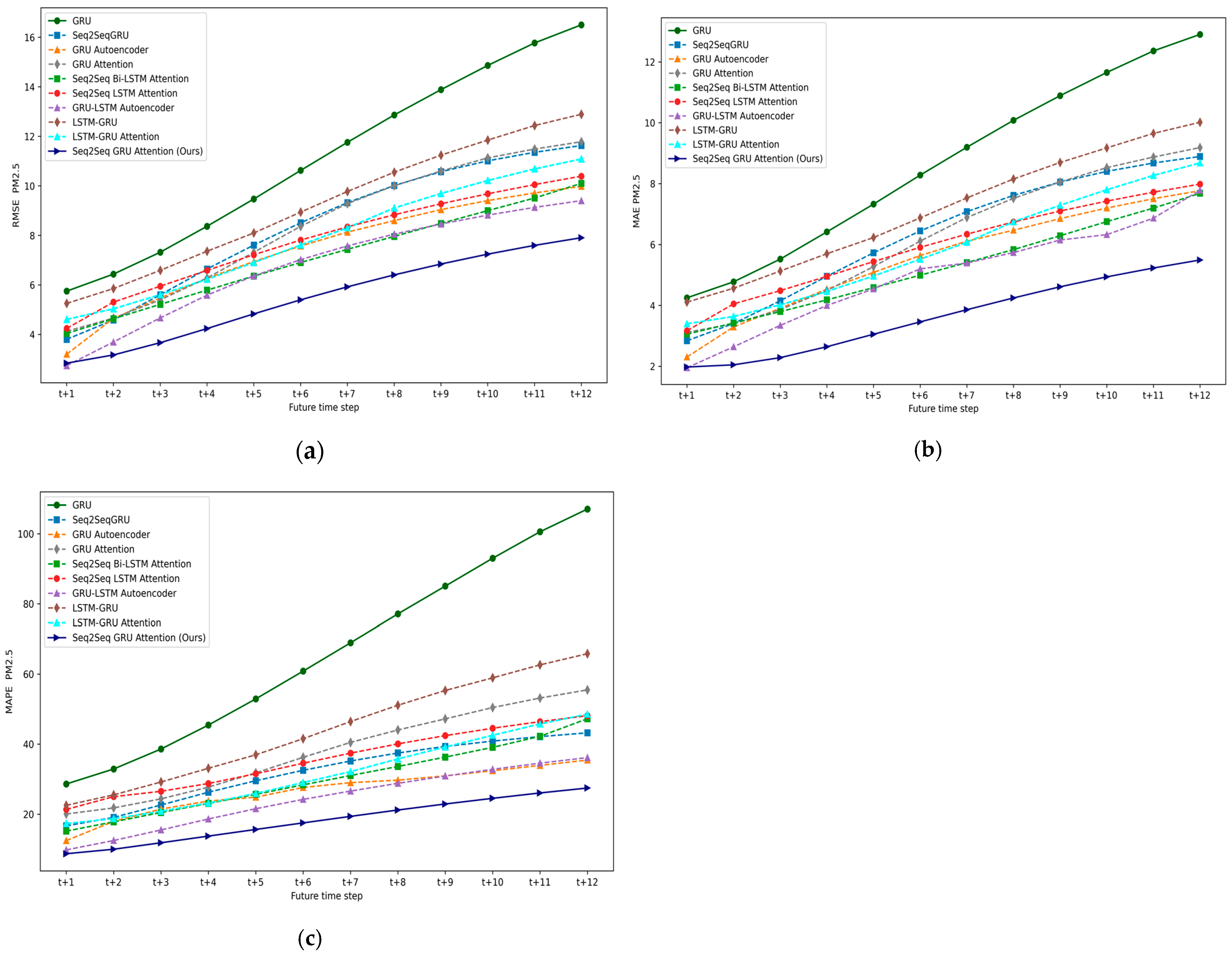
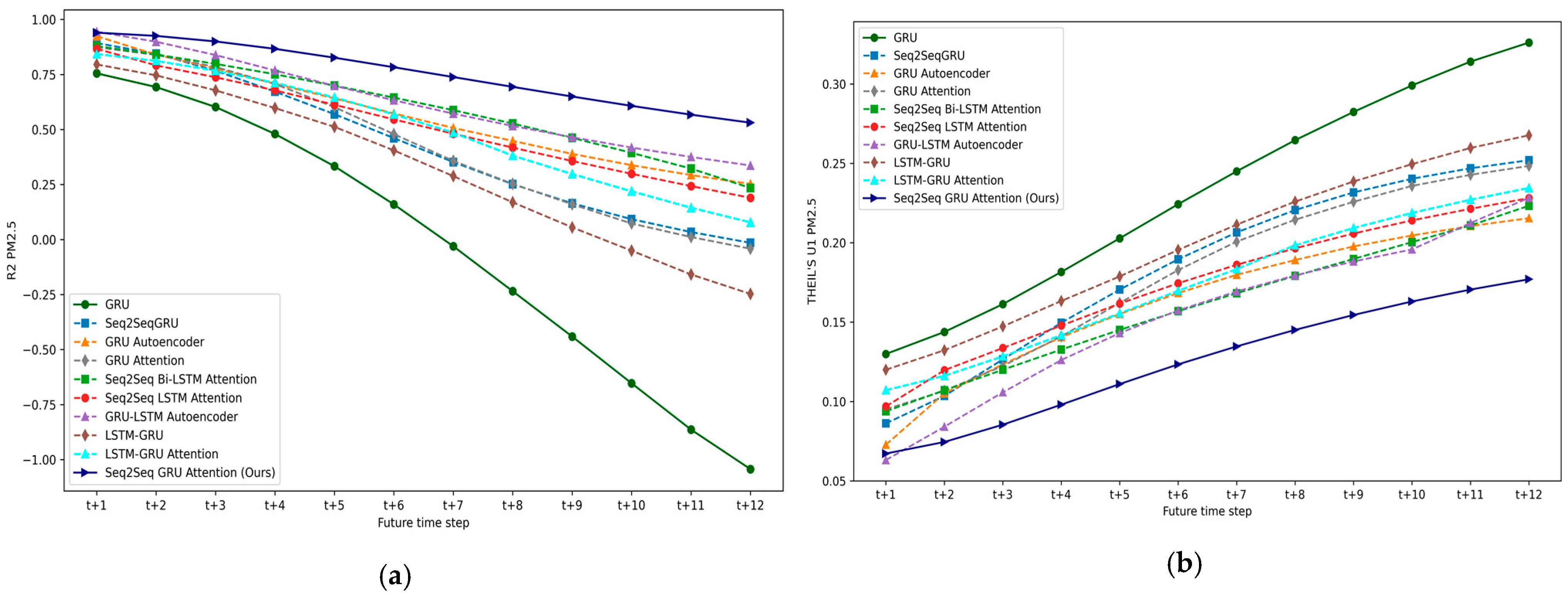
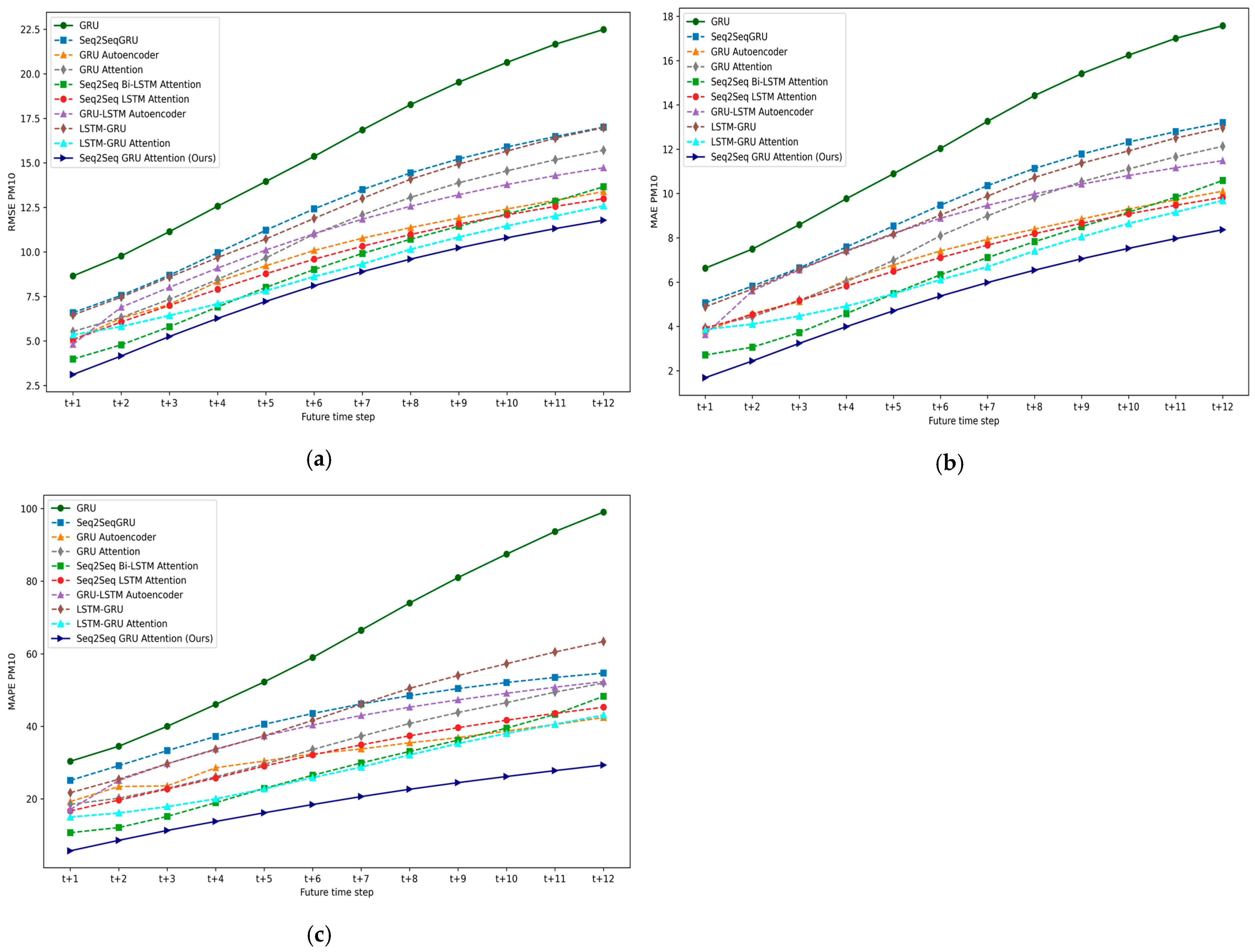
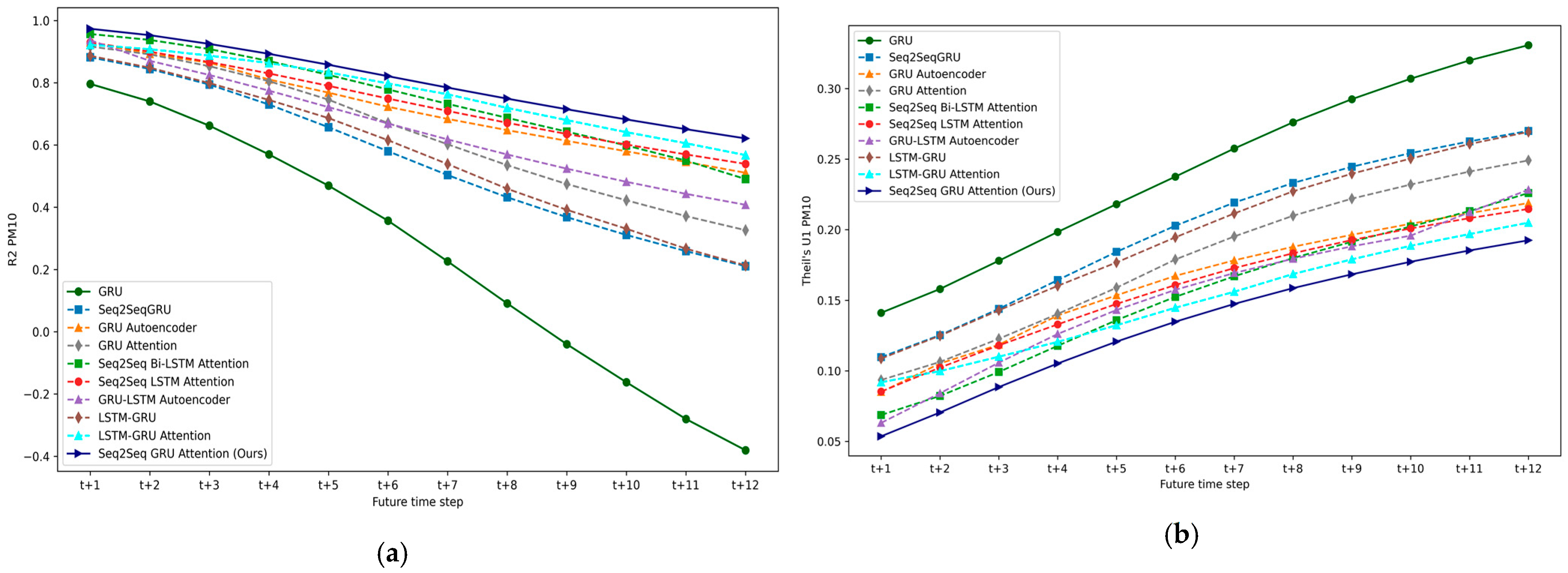
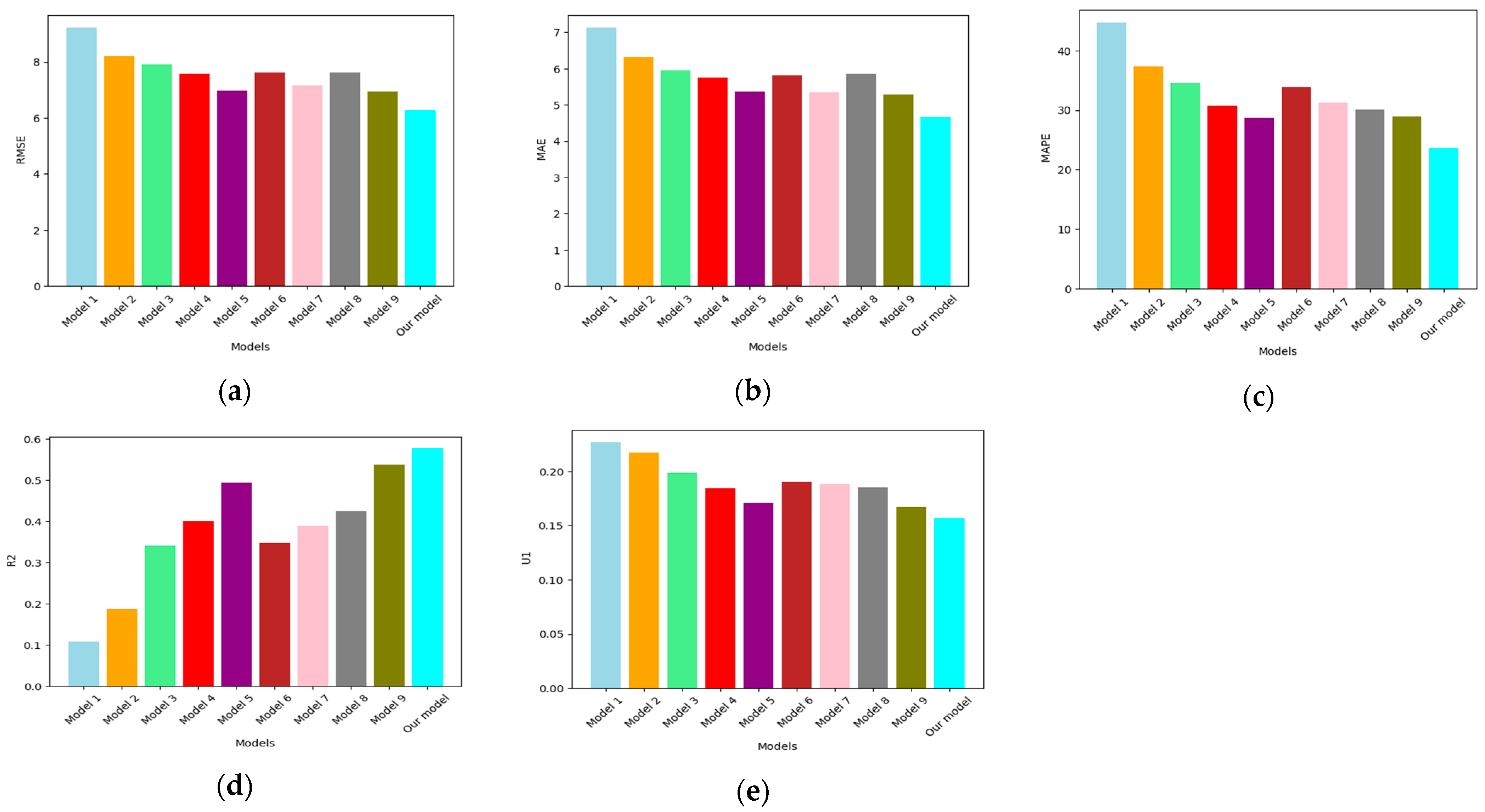
- The traditional RNN model, GRU, exhibited the least average forecasting performance with an RMSE, MAE, MAPE, R2, and Theil’s U1 of 9.2129, 7.1219, 44.63, 0.081, and 0.2268, respectively. Moreover, the effectiveness of the GRU is improved through a hybrid RNN approach like the LSTM-GRU, which demonstrates better performance. Compared to the GRU, a hybrid LSTM-GRU has a better average forecasting performance across all the pollutants, where RMSE, MAE, MAPE, and Theil’s U1 are decreased by 10.89%, 11.32%, 16.54%, and 4.32%, respectively, while R2 is increased by 0.1052.
- Seq2Seq GRU exhibited improved average forecasting performance over the RNN variants (LSTM-GRU and GRU). This indicates that introducing an encoder–decoder into the RNN model is beneficial to enhance the forecasting performance. For instance, compared with the LSTM-GRU, the RMSE of Seq2Seq GRU decreases by 3.19%, the MAE decreases by 5.79%, MAPE decreases by 7.38%, Theil’s U1 decreases by 9.19%, and R2 increases by 0.1553.
- The forecasting performance of the Autoencoder model (GRU Autoencoder), a variant of the encoder–decoder is superior to the Seq2Seq GRU for all the pollutants. Despite this, the hybrid variant of AE (GRU-LSTM Autoencoder) has better performance than the GRU-AE. Compared with the GRU Autoencoder, the RMSE, MAE, MAPE, and Theil’s U1 of the GRU-LSTM Autoencoder decrease by 8.81%, 6.76%, 7.06%, and 7.24% respectively, and R2 increases by 0.0931.
- Moreover, adding an attention mechanism to the LSTM-GRU architecture, as seen in the LSTM-GRU Attention, led to an enhancement in forecasting performance. Compared with the LSTM-GRU, the RMSE, MAE, MAPE, and Theil’s U1 of the LSTM-GRU Attention model decrease by 12.76%, 15.45%, 19.23%, and 15.14%, respectively, and R2 is increased by 0.2022. The encoder–decoder-based attention variants (Seq2Seq LSTM Attention, Seq2Seq Bi-LSTM Attention, and Seq2Seq GRU Attention) exhibit improved performance over the Seq2Seq GRU. This indicates that introducing an attention mechanism overcomes the limitations of the traditional Seq2seq RNN models by dynamically focusing on relevant input sequences to capture contextual information critical for accurate predictions, mitigating information loss from fixed-length context vectors, addressing the vanishing gradient problem for effectively capturing long-range dependencies, and generating context-related forecasts with enhanced performance.
- The Seq2Seq Bi-LSTM Attention exhibits a similar average forecasting performance compared to the GRU-LSTM Autoencoder; the latter demonstrates better efficacy specifically for the pollutants PM2.5, NO2, and O3. However, the proposed Seq2Seq GRU Attention model demonstrates the best average performance across twelve time steps for each of the pollutants, as well as superior average forecasting performance across all the pollutants in comparison with the baselines. Compared with the Seq2Seq Bi-LSTM Attention, the average forecasting performance of the proposed model across all the pollutants in terms of RMSE decreases by 18.27%, MAE decreases by 33.83%, MAPE decreases by 33.51%, Theil’s U1 decreases by 18.95%, and R2 increases by 28.70%.
- The proposed Seq2Seq GRU Attention achieves the best average forecasting performance across six pollutants for 12 time steps, with an average RMSE of 5.5576, MAE of 3.4975, MAPE of 19.1991, R2 of 0.6926, and Theil’s U1 of 0.6926, as highlighted in bold in Table 10.
5.2. Experiment II: Evaluation of an Optimized Lightweight DL Model for Efficient Fog Intelligence
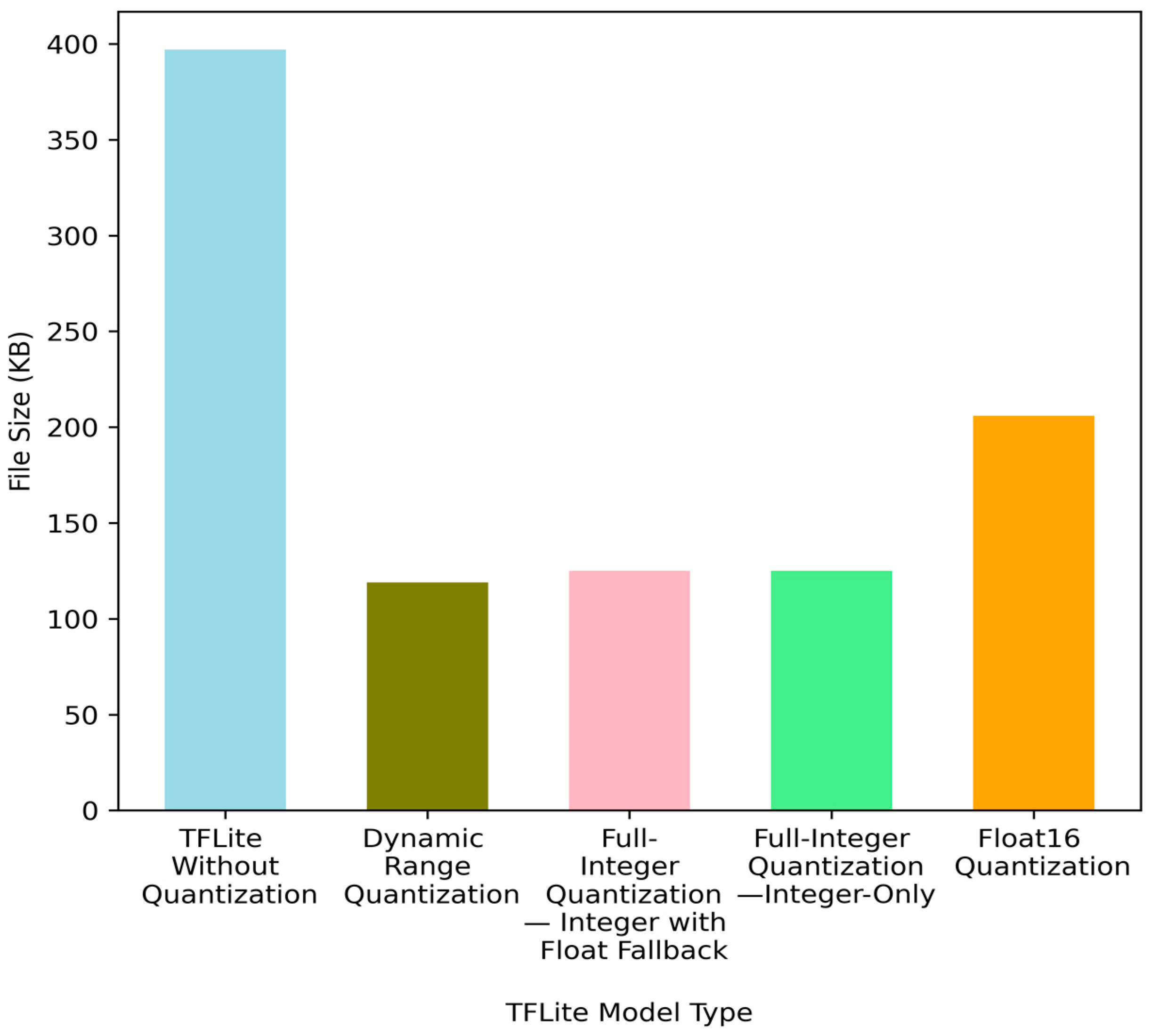
- TFLite converter: The TFLite converter converts TF models into an optimized format by applying optimization techniques such as quantization, model pruning, and operator fusion to reduce model size and increase inference speed. It generates a TensorFlow Lite model file (.tflite) that contains the converted model in a format that the TFLite interpreter can handle.
- TFLite interpreter: The TFLite interpreter loads the TFLite model (optimized model), prepares it for execution, and enables on-device inferencing using the input data. It enables the efficient execution of TFLite models.
6. Conclusions and Future Works
Author Contributions
Funding
Institutional Review Board Statement
Informed Consent Statement
Data Availability Statement
Conflicts of Interest
References
- Bakır, H.; Ağbulut, Ü.; Gürel, A.E.; Yıldız, G.; Güvenç, U.; Soudagar, M.E.M.; Hoang, A.T.; Deepanraj, B.; Saini, G.; Afzal, A. Forecasting of Future Greenhouse Gas Emission Trajectory for India Using Energy and Economic Indexes with Various Metaheuristic Algorithms. J. Clean. Prod. 2022, 360, 131946. [Google Scholar] [CrossRef]
- Air Pollution and Health | UNECE. Available online: https://unece.org/air-pollution-and-health (accessed on 5 January 2023).
- Yuan, L.; Li, H.; Fu, S.; Zhang, Z. Learning Behavior Evaluation Model and Teaching Strategy Innovation by Social Media Network Following Learning Psychology. Front. Psychol. 2022, 13, 843428. [Google Scholar] [CrossRef] [PubMed]
- Wu, X.; Nethery, R.C.; Sabath, M.B.; Braun, D.; Dominici, F. Air Pollution and COVID-19 Mortality in the United States: Strengths and Limitations of an Ecological Regression Analysis. Sci. Adv. 2020, 6, eabd4049. [Google Scholar] [CrossRef] [PubMed]
- Pekdogan, T.; Udriștioiu, M.T.; Yildizhan, H.; Ameen, A. From Local Issues to Global Impacts: Evidence of Air Pollution for Romania and Turkey. Sensors 2024, 24, 1320. [Google Scholar] [CrossRef] [PubMed]
- Georgiev, D. Internet of Things Statistics, Facts & Predictions [2024’s Update]. Available online: https://review42.com/resources/internet-of-things-stats/ (accessed on 13 January 2024).
- Bharathi, P.D.; Ananthanarayanan, V.; Sivakumar, P.B. Fog Computing-Based Environmental Monitoring Using Nordic Thingy: 52 and Raspberry Pi. In Smart Innovation, Systems and Technologies; Springer: Singapore, 2019; pp. 269–279. [Google Scholar]
- Losada, M.; Cortés, A.; Irizar, A.; Cejudo, J.; Pérez, A. A Flexible Fog Computing Design for Low-Power Consumption and Low Latency Applications. Electronics 2020, 10, 57. [Google Scholar] [CrossRef]
- Brogi, A.; Forti, S.; Guerrero, C.; Lera, I. How to Place Your Apps in the Fog: State of the Art and Open Challenges. Softw. Pract. Exp. 2019, 50, 719–740. [Google Scholar] [CrossRef]
- Daraghmi, Y.-A.; Daraghmi, E.Y.; Daraghma, R.; Fouchal, H.; Ayaida, M. Edge–Fog–Cloud Computing Hierarchy for Improving Performance and Security of NB-IoT-Based Health Monitoring Systems. Sensors 2022, 22, 8646. [Google Scholar] [CrossRef] [PubMed]
- Yousefpour, A.; Patil, A.; Ishigaki, G.; Kim, I.; Wang, X.; Cankaya, H.C.; Zhang, Q.; Xie, W.; Jue, J.P. FOGPLAN: A Lightweight QoS-Aware Dynamic Fog Service Provisioning Framework. IEEE Internet Things J. 2019, 6, 5080–5096. [Google Scholar] [CrossRef]
- Himeur, Y.; Sayed, A.N.; Alsalemi, A.; Bensaali, F.; Amira, A. Edge AI for Internet of Energy: Challenges and Perspectives. Internet Things 2024, 25, 101035. [Google Scholar] [CrossRef]
- Peruzzi, G.; Pozzebon, A. Combining LoRaWAN and NB-IoT for Edge-to-Cloud Low Power Connectivity Leveraging on Fog Computing. Appl. Sci. 2022, 12, 1497. [Google Scholar] [CrossRef]
- Fraga-Lamas, P.; Celaya-Echarri, M.; Lopez-Iturri, P.; Castedo, L.; Azpilicueta, L.; Aguirre, E.; Suárez-Albela, M.; Falcone, F.; Fernández-Caramés, T.M. Design and Experimental Validation of a LoRaWAN Fog Computing Based Architecture for IoT Enabled Smart Campus Applications. Sensors 2019, 19, 3287. [Google Scholar] [CrossRef] [PubMed]
- Bharathi, P.D.; Narayanan, V.A.; Sivakumar, P.B. Fog Computing Enabled Air Quality Monitoring and Prediction Leveraging Deep Learning in IoT. J. Intell. Fuzzy Syst. 2022, 43, 5621–5642. [Google Scholar] [CrossRef]
- National Air Quality Index. Available online: https://cpcb.nic.in/displaypdf.php?id=bmF0aW9uYWwtYWlyLXF1YWxpdHktaW5kZXgvQWJvdXRfQVFJLnBkZg== (accessed on 18 January 2023).
- Grace, R.K.; Manju, S. A Comprehensive Review of Wireless Sensor Networks Based Air Pollution Monitoring Systems. Wirel. Pers. Commun. 2019, 108, 2499–2515. [Google Scholar] [CrossRef]
- Dhingra, S.; Madda, R.B.; Gandomi, A.H.; Patan, R.; Daneshmand, M. Internet of Things Mobile–Air Pollution Monitoring System (IoT-Mobair). IEEE Internet Things J. 2019, 6, 5577–5584. [Google Scholar] [CrossRef]
- Laskar, M.R.; Sen, P.K.; Mandal, S.K.D. An IoT-Based e-Health System Integrated With Wireless Sensor Network and Air Pollution Index. In Proceedings of the 2019 Second International Conference on Advanced Computational and Communication Paradigms (ICACCP), Gangtok, India, 25–28 February 2019. [Google Scholar] [CrossRef]
- Alam, S.S.; Islam, A.J.; Hasan, M.; Rafid, M.N.M.; Chakma, N.; Imtiaz, N. Design and Development of a Low-Cost IoT Based Environmental Pollution Monitoring System. In Proceedings of the 2018 4th International Conference on Electrical Engineering and Information & Communication Technology (iCEEiCT), Dhaka, Bangladesh, 13–15 September 2018. [Google Scholar] [CrossRef]
- Kelechi, A.H.; Alsharif, M.H.; Agbaetuo, C.; Ubadike, O.; Aligbe, A.; Uthansakul, P.; Kannadasan, R.; Aly, A.A. Design of a Low-Cost Air Quality Monitoring System Using Arduino and ThingSpeak. Comput. Mater. Contin. Comput. Mater. Contin. 2022, 70, 151–169. [Google Scholar] [CrossRef]
- Kumar, T.; Doss, A. AIRO: Development of an Intelligent IoT-Based Air Quality Monitoring Solution for Urban Areas. Procedia Comput. Sci. 2023, 218, 262–273. [Google Scholar] [CrossRef]
- Bobulski, J.; Szymoniak, S.; Pasternak, K. An IoT System for Air Pollution Monitoring with Safe Data Transmission. Sensors 2024, 24, 445. [Google Scholar] [CrossRef] [PubMed]
- Kairuz-Cabrera, D.; Hernandez-Rodriguez, V.; Schalm, O.; Laguardia, A.M.; Laso, P.M.; Sánchez, D.A. Development of a Unified IoT Platform for Assessing Meteorological and Air Quality Data in a Tropical Environment. Sensors 2024, 24, 2729. [Google Scholar] [CrossRef] [PubMed]
- Asha, P.; Natrayan, L.; Geetha, B.T.; Beulah, J.R.; Sumathy, R.; Varalakshmi, G.; Neelakandan, S. IoT Enabled Environmental Toxicology for Air Pollution Monitoring Using AI Techniques. Environ. Res. 2022, 205, 112574. [Google Scholar] [CrossRef]
- Arroyo, P.; Gómez-Suárez, J.; Suárez, J.I.; Lozano, J. Low-Cost Air Quality Measurement System Based on Electrochemical and PM Sensors with Cloud Connection. Sensors 2021, 21, 6228. [Google Scholar] [CrossRef]
- Barthwal, A. A Markov Chain–Based IoT System for Monitoring and Analysis of Urban Air Quality. Environ. Monit. Assess. 2022, 195, 235. [Google Scholar] [CrossRef] [PubMed]
- Samad, A.; Kieser, J.; Chourdakis, I.; Vogt, U. Developing a Cloud-Based Air Quality Monitoring Platform Using Low-Cost Sensors. Sensors 2024, 24, 945. [Google Scholar] [CrossRef]
- Binsy, M.S.; Sampath, N. User Configurable and Portable Air Pollution Monitoring System for Smart Cities Using IoT. In International Conference on Computer Networks and Communication Technologies; Lecture Notes on Data Engineering and Communications Technologies; Springer: Singapore, 2018; pp. 345–359. [Google Scholar]
- Palomeque-Mangut, S.; Meléndez, F.; Gómez-Suárez, J.; Frutos-Puerto, S.; Arroyo, P.; Pinilla-Gil, E.; Lozano, J. Wearable System for Outdoor Air Quality Monitoring in a WSN with Cloud Computing: Design, Validation and Deployment. Chemosphere 2022, 307, 135948. [Google Scholar] [CrossRef] [PubMed]
- Koziel, S.; Pietrenko-Dabrowska, A.; Wojcikowski, M.; Pankiewicz, B. Efficient Calibration of Cost-Efficient Particulate Matter Sensors Using Machine Learning and Time-Series Alignment. Knowl.-Based Syst. 2024, 295, 111879. [Google Scholar] [CrossRef]
- Koziel, S.; Pietrenko-Dabrowska, A.; Wojcikowski, M.; Pankiewicz, B. Field Calibration of Low-Cost Particulate Matter Sensors Using Artificial Neural Networks and Affine Response Correction. Measurement 2024, 230, 114529. [Google Scholar] [CrossRef]
- Lai, X.; Yang, T.; Wang, Z.; Chen, P. IoT Implementation of Kalman Filter to Improve Accuracy of Air Quality Monitoring and Prediction. Appl. Sci. 2019, 9, 1831. [Google Scholar] [CrossRef]
- Moursi, A.S.; El-Fishawy, N.; Djahel, S.; Shouman, M.A. An IoT Enabled System for Enhanced Air Quality Monitoring and Prediction on the Edge. Complex Intell. Syst. 2021, 7, 2923–2947. [Google Scholar] [CrossRef] [PubMed]
- Kristiani, E.; Yang, C.-T.; Huang, C.-Y.; Wang, Y.-T.; Ko, P.-C. The Implementation of a Cloud-Edge Computing Architecture Using OpenStack and Kubernetes for Air Quality Monitoring Application. J. Spec. Top. Mob. Netw. Appl. Mob. Netw. Appl. 2020, 26, 1070–1092. [Google Scholar] [CrossRef]
- Senthilkumar, R.; Venkatakrishnan, P.; Balaji, N. Intelligent Based Novel Embedded System Based IoT Enabled Air Pollution Monitoring System. Microprocess. Microsyst. 2020, 77, 103172. [Google Scholar] [CrossRef]
- Santos, J.; Leroux, P.; Wauters, T.; Volckaert, B.; De Turck, F. Anomaly Detection for Smart City Applications over 5G Low Power Wide Area Networks. In Proceedings of the NOMS 2018—2018 IEEE/IFIP Network Operations and Management Symposium, Taipei, Taiwan, 23–27 April 2018. [Google Scholar] [CrossRef]
- Jabbar, W.A.; Subramaniam, T.; Ong, A.E.; Shu’Ib, M.I.; Wu, W.; De Oliveira, M.A. LoRaWAN-Based IoT System Implementation for Long-Range Outdoor Air Quality Monitoring. Internet Things 2022, 19, 100540. [Google Scholar] [CrossRef]
- Moses, L.; Tamilselvan, N.; Raju, N.; Karthikeyan, N. IoT Enabled Environmental Air Pollution Monitoring and Rerouting System Using Machine Learning Algorithms. IOP Conf. Series. Mater. Sci. Eng. 2020, 955, 012005. [Google Scholar] [CrossRef]
- Manalu, I.P.; Silalahi, S.M.; Wowiling, G.I.; Sigiro, M.M.T.; Zalukhu, R.P.; Nababan, P.K. Lora Communication Design and Performance Test (Case Study: Air Quality Monitoring System). In Proceedings of the 2023 International Conference of Computer Science and Information Technology (ICOSNIKOM), Binjia, Indonesia, 10–11 November 2023. [Google Scholar] [CrossRef]
- Nalakurthi, N.V.S.R.; Abimbola, I.; Ahmed, T.; Anton, I.; Riaz, K.; Ibrahim, Q.; Banerjee, A.; Tiwari, A.; Gharbia, S. Challenges and Opportunities in Calibrating Low-Cost Environmental Sensors. Sensors 2024, 24, 3650. [Google Scholar] [CrossRef] [PubMed]
- Pant, A.; Joshi, R.C.; Sharma, S.; Pant, K. Predictive Modeling for Forecasting Air Quality Index (AQI) Using Time Series Analysis. Avicenna J. Environ. Health Eng. 2023, 10, 38–43. [Google Scholar] [CrossRef]
- Castelli, M.; Clemente, F.M.; Popovič, A.; Silva, S.; Vanneschi, L. A Machine Learning Approach to Predict Air Quality in California. Complexity 2020, 2020, 8049504. [Google Scholar] [CrossRef]
- Doreswamy, S.H.K.; Km, Y.; Gad, I. Forecasting Air Pollution Particulate Matter (PM2.5) Using Machine Learning Regression Models. Procedia Comput. Sci. 2020, 171, 2057–2066. [Google Scholar] [CrossRef]
- Liang, Y.-C.; Maimury, Y.; Chen, A.H.-L.; Juarez, J.R.C. Machine Learning-Based Prediction of Air Quality. Appl. Sci. 2020, 10, 9151. [Google Scholar] [CrossRef]
- Zhu, D.; Cai, C.; Yang, T.; Zhou, X. A Machine Learning Approach for Air Quality Prediction: Model Regularization and Optimization. Big Data Cogn. Comput. 2018, 2, 5. [Google Scholar] [CrossRef]
- Dairi, A.; Harrou, F.; Khadraoui, S.; Sun, Y. Integrated Multiple Directed Attention-Based Deep Learning for Improved Air Pollution Forecasting. IEEE Trans. Instrum. Meas. 2021, 70, 3520815. [Google Scholar] [CrossRef]
- Jiao, Y.; Wang, Z.; Zhang, Y. Prediction of Air Quality Index Based on LSTM. In Proceedings of the 2019 IEEE 8th Joint International Information Technology and Artificial Intelligence Conference (ITAIC), Chongqing, China, 24–26 May 2019. [Google Scholar] [CrossRef]
- Wang, X.; Yan, J.; Wang, X.; Wang, Y. Air Quality Forecasting Using the GRU Model Based on Multiple Sensors Nodes. IEEE Sens. Lett. 2023, 7, 6003804. [Google Scholar] [CrossRef]
- Rao, K.S.; Devi, G.L.; Ramesh, N. Air Quality Prediction in Visakhapatnam with LSTM Based Recurrent Neural Networks. Int. J. Intell. Syst. Appl. 2019, 11, 18–24. [Google Scholar] [CrossRef]
- Belavadi, S.V.; Rajagopal, S.; Ranjani, R.; Mohan, R. Air Quality Forecasting Using LSTM RNN and Wireless Sensor Networks. Procedia Comput. Sci. 2020, 170, 241–248. [Google Scholar] [CrossRef]
- Fang, W.; Zhu, R.; Lin, J.C.-W. An Air Quality Prediction Model Based on Improved Vanilla LSTM with Multichannel Input and Multiroute Output. Expert Syst. Appl. 2023, 211, 118422. [Google Scholar] [CrossRef]
- Middya, A.I.; Roy, S. Pollutant Specific Optimal Deep Learning and Statistical Model Building for Air Quality Forecasting. Soc. Sci. Res. Netw. 2022, 301, 118972. [Google Scholar] [CrossRef]
- Athira, V.; Geetha, P.; Vinayakumar, R.; Soman, K.P. DeepAirNet: Applying Recurrent Networks for Air Quality Prediction. Procedia Comput. Sci. 2018, 132, 1394–1403. [Google Scholar] [CrossRef]
- Lin, C.-Y.; Chang, Y.-S.; Abimannan, S. Ensemble Multifeatured Deep Learning Models for Air Quality Forecasting. Atmos. Pollut. Res. 2021, 12, 101045. [Google Scholar] [CrossRef]
- Liu, H.; Yan, G.; Duan, Z.; Chen, C. Intelligent Modeling Strategies for Forecasting Air Quality Time Series: A Review. Appl. Soft Comput. 2021, 102, 106957. [Google Scholar] [CrossRef]
- Sarkar, N.; Gupta, R.; Keserwani, P.K.; Govil, M.C. Air Quality Index Prediction Using an Effective Hybrid Deep Learning Model. Environ. Pollut. 2022, 315, 120404. [Google Scholar] [CrossRef]
- Huang, C.-J.; Kuo, P.-H. A Deep CNN-LSTM Model for Particulate Matter (PM2.5) Forecasting in Smart Cities. Sensors 2018, 18, 2220. [Google Scholar] [CrossRef]
- Sharma, E.; Deo, R.C.; Soar, J.; Prasad, R.; Parisi, A.V.; Raj, N. Novel Hybrid Deep Learning Model for Satellite Based PM10 Forecasting in the Most Polluted Australian Hotspots. Atmos. Environ. 2022, 279, 119111. [Google Scholar] [CrossRef]
- Yeo, I.; Choi, Y.; Lops, Y.; Sayeed, A. Efficient PM2.5 Forecasting Using Geographical Correlation Based on Integrated Deep Learning Algorithms. Neural Comput. Appl. 2021, 33, 15073–15089. [Google Scholar] [CrossRef]
- Yang, Y.; Mei, G.; Izzo, S. Revealing Influence of Meteorological Conditions on Air Quality Prediction Using Explainable Deep Learning. IEEE Access 2022, 10, 50755–50773. [Google Scholar] [CrossRef]
- Chang, Y.-S.; Chiao, H.-T.; Abimannan, S.; Huang, Y.-P.; Tsai, Y.-T.; Lin, K.-M. An LSTM-Based Aggregated Model for Air Pollution Forecasting. Atmos. Pollut. Res. 2020, 11, 1451–1463. [Google Scholar] [CrossRef]
- Du, S.; Li, T.; Yang, Y.; Horng, S.-J. Deep Air Quality Forecasting Using Hybrid Deep Learning Framework. IEEE Trans. Knowl. Data Eng. 2021, 33, 2412–2424. [Google Scholar] [CrossRef]
- Kow, P.-Y.; Wang, Y.-S.; Zhou, Y.; Kao, I.-F.; Issermann, M.; Chang, L.-C.; Chang, F.-J. Seamless Integration of Convolutional and Back-Propagation Neural Networks for Regional Multi-Step-Ahead PM2.5 Forecasting. J. Clean. Prod. 2020, 261, 121285. [Google Scholar] [CrossRef]
- Janarthanan, R.; Partheeban, P.; Somasundaram, K.; Elamparithi, P.N. A Deep Learning Approach for Prediction of Air Quality Index in a Metropolitan City. Sustain. Cities Soc. 2021, 67, 102720. [Google Scholar] [CrossRef]
- Al-Janabi, S.; Alkaim, A.; Al-Janabi, E.; Aljeboree, A.; Mustafa, M. Intelligent Forecaster of Concentrations (PM2.5, PM10, NO2, CO, O3, SO2) Caused Air Pollution (IFCsAP). Neural Comput. Appl. 2021, 33, 14199–14229. [Google Scholar] [CrossRef]
- Mokhtari, I.; Bechkit, W.; Rivano, H.; Yaici, M.R. Uncertainty-Aware Deep Learning Architectures for Highly Dynamic Air Quality Prediction. IEEE Access 2021, 9, 14765–14778. [Google Scholar] [CrossRef]
- Hu, K.; Guo, X.; Gong, X.; Wang, X.; Liang, J.; Li, D. Air Quality Prediction Using Spatio-Temporal Deep Learning. Atmos. Pollut. Res. 2022, 13, 101543. [Google Scholar] [CrossRef]
- Feng, H.; Zhang, X. A Novel Encoder-Decoder Model Based on Autoformer for Air Quality Index Prediction. PLoS ONE 2023, 18, e0284293. [Google Scholar] [CrossRef]
- Zhang, B.; Zou, G.; Qin, D.; Lu, Y.; Jin, Y.; Wang, H. A Novel Encoder-Decoder Model Based on Read-First LSTM for Air Pollutant Prediction. Sci. Total Environ. 2021, 765, 144507. [Google Scholar] [CrossRef]
- Alhnaity, B.; Kollias, S.; Leontidis, G.; Jiang, S.; Schamp, B.; Pearson, S. An Autoencoder Wavelet Based Deep Neural Network with Attention Mechanism for Multi-Step Prediction of Plant Growth. Inf. Sci. 2021, 560, 35–50. [Google Scholar] [CrossRef]
- Feng, L.; Zhao, C.; Sun, Y. Dual Attention-Based Encoder–Decoder: A Customized Sequence-to-Sequence Learning for Soft Sensor Development. IEEE Trans. Neural Netw. Learn. Syst. 2021, 32, 3306–3317. [Google Scholar] [CrossRef]
- Chen, Z.; Yu, H.; Geng, Y.-A.; Li, Q.; Zhang, Y. EvaNet: An Extreme Value Attention Network for Long-Term Air Quality Prediction. In Proceedings of the 2020 IEEE International Conference on Big Data (Big Data), Atlanta, GA, USA, 10–13 December 2020. [Google Scholar] [CrossRef]
- Li, S.; Xie, G.; Ren, J.; Guo, L.; Yang, Y.; Xu, X. Urban PM2.5 Concentration Prediction via Attention-Based CNN–LSTM. Appl. Sci. 2020, 10, 1953. [Google Scholar] [CrossRef]
- Du, S.; Li, T.; Yang, Y.; Horng, S.-J. Multivariate Time Series Forecasting via Attention-Based Encoder–Decoder Framework. Neurocomputing 2020, 388, 269–279. [Google Scholar] [CrossRef]
- Jia, P.; Cao, N.; Yang, S. Real-Time Hourly Ozone Prediction System for Yangtze River Delta Area Using Attention Based on a Sequence to Sequence Model. Atmos. Environ. 2021, 244, 117917. [Google Scholar] [CrossRef]
- Blogs. Available online: https://community.intel.com/t5/Blogs/ct-p/blogs/ai-inference-at-scale#gs.6ojv36 (accessed on 10 February 2023).
- Andrade, P.; Silva, I.; Silva, M.; Flores, T.; Cassiano, J.; Costa, D.G. A TinyML Soft-Sensor Approach for Low-Cost Detection and Monitoring of Vehicular Emissions. Sensors 2022, 22, 3838. [Google Scholar] [CrossRef]
- Maccantelli, F.; Peruzzi, G.; Pozzebon, A. Traffic Level Monitoring in Urban Scenarios with Virtual Sensing Techniques Enabled by Embedded Machine Learning. In Proceedings of the 2023 IEEE Sensors Applications Symposium (SAS), Ottawa, ON, Canada, 18–20 July 2023. [Google Scholar] [CrossRef]
- Liu, D.; Kong, H.; Luo, X.; Liu, W.; Subramaniam, R. Bringing AI to Edge: From Deep Learning’s Perspective. Neurocomputing 1507 2022, 485, 297–320. [Google Scholar] [CrossRef]
- Post-Training Quantization. Available online: https://www.tensorflow.org/lite/performance/post_training_quantization (accessed on 15 June 2023).
- Lee, H.; Lee, N.; Lee, S. A Method of Deep Learning Model Optimization for Image Classification on Edge Device. Sensors 2022, 22, 7344. [Google Scholar] [CrossRef]
- Shuvo, M.M.H.; Islam, S.K.; Cheng, J.; Morshed, B.I. Efficient Acceleration of Deep Learning Inference on Resource-Constrained Edge Devices: A Review. Proc. IEEE 2023, 111, 42–91. [Google Scholar] [CrossRef]
- Lalapura, V.S.; Amudha, J.; Satheesh, H.S. Recurrent Neural Networks for Edge Intelligence. ACM Comput. Surv. 2021, 54, 91. [Google Scholar] [CrossRef]
- Merenda, M.; Porcaro, C.; Iero, D. Edge Machine Learning for AI-Enabled IoT Devices: A Review. Sensors 2020, 20, 2533. [Google Scholar] [CrossRef]
- Yao, J.; Zhang, S.; Yao, Y.; Wang, F.; Ma, J.; Zhang, J.; Chu, Y.; Ji, L.; Jia, K.; Shen, T.; et al. Edge-Cloud Polarization and Collaboration: A Comprehensive Survey for AI. IEEE Trans. Knowl. Data Eng. 2022, 1, 6866–6886. [Google Scholar] [CrossRef]
- Polino, A.; Pascanu, R.; Alistarh, D. Model Compression via Distillation and Quantization. arXiv 2018. [Google Scholar] [CrossRef]
- MQ136 Datasheet. Available online: https://pdf1.alldatasheet.com/datasheet-pdf/view/1131997/hanwei/mq-136.html (accessed on 6 February 2023).
- Makhija, J.; Nakkeeran, M.; Narayanan, V.A. Detection of Vehicle Emissions Through Green IoT for Pollution Control. In Advances in Automation, Signal Processing, Instrumentation, and Control; Lecture Notes in Electrical Engineering; Springer: Singapore, 2021; pp. 817–826. [Google Scholar] [CrossRef]
- Gorospe, J.; Mulero, R.; Arbelaitz, O.; Muguerza, J.; Antón, M.Á. A Generalization Performance Study Using Deep Learning Networks in Embedded Systems. Sensors 2021, 21, 1031. [Google Scholar] [CrossRef]
- Eren, B.; Aksangür, İ.; Erden, C. Predicting next Hour Fine Particulate Matter (PM2.5) in the Istanbul Metropolitan City Using Deep Learning Algorithms with Time Windowing Strategy. Urban Clim. 2023, 48, 101418. [Google Scholar] [CrossRef]
- He, Y.-L.; Chen, L.; Gao, Y.; Ma, J.-H.; Xu, Y.; Zhu, Q.-X. Novel Double-Layer Bidirectional LSTM Network with Improved Attention Mechanism for Predicting Energy Consumption. ISA Trans. 2022, 127, 350–360. [Google Scholar] [CrossRef] [PubMed]
- Central Control Room for Air Quality Management—All India, CPCB. Available online: https://airquality.cpcb.gov.in/ccr/#/caaqm-dashboard-all/caaqm-landing/caaqm-data-repository (accessed on 23 January 2023).


| AQI | Descriptor | Indicative Color | Associated Health Impacts |
|---|---|---|---|
| 0 to 50 | Good | Green | Poses minimal or no risk |
| 51 to 100 | Satisfactory | Yellow | Acceptable air quality level. Minor concern for the sensitive members of the population |
| 101 to 200 | Moderately Polluted | Orange | Sensitive members of the population may experience health effects from prolonged exposure. |
| 201 to 300 | Poor | Red | The public may start to experience illness. Severe effect on the sensitive members of the population. |
| 301 to 400 | Very poor | Purple | Health alert. Serious health impacts for everyone. |
| 401 to 500 | Severe | Maroon | Emergency warning. Everyone is likely to be affected. |
| Reference | Pollutants Monitored | Controllers, Sensors, and Other Hardware Platforms | Meteorological Parameters | Edge/Fog Computing | LPWAN | Cloud Computing | Air Quality Forecasting | Optimized DL Model-Fog Intelligence | Early Warnings | Web Application |
|---|---|---|---|---|---|---|---|---|---|---|
| Laskar et al. [22] | CO, CO2, PM2.5, PM10, SO2, NO2 | ESP8266, MQ2, MQ 7, MQ131, MQ135, MQ 136 | X | X | X | √ | X | X | X | √ |
| Kumar et al. [25] | PM10, PM2.5, NO2, CO2 | Intel Edison, GPS, MQ131, MQ135, MQ136, MQ7 sensors | X | X | X | √ | √ | X | √ | √ |
| Aashiq et al. [28] | PM2.5, PM10, VOC, CO, Temperature, Pressure, Humidity, Altitude | Arduino Uno, ESP 8266, BMP280, AHT10, MQ7 | √ | X | X | √ | X | X | X | √ |
| Asha et al. [29] | PM2.5, CO, CO2, NH3, NO2, CH4, Temperature, Humidity | Grove-Multichannel Gas Sensor, MHZ19, DHT11, HM3301 laser, PM2.5 sensor | √ | X | X | √ | √ | X | √ | X |
| Moses et al. [39] | PM2.5, PM10, CO, O3, NO2, SO2. | MQ136, MQ7, RPi 3, PM2.5 sensor, NO2 sensor, O3 sensor, NB-IoT. | X | X | √ | √ | √ | X | X | √ |
| Lai X et al. [33] | PM2.5, PM10, SO2, NO2, CO, O3 | ESP8266, Raspberry Pi 3 Model B, ZH03A, SGA-700 Intelligent Gas Sensor | X | √ | X | √ | √ | X | X | √ |
| Senthilkumar et al. [34] | PM2.5, PM10, SO2, NO2, CO, O3 | GP2Y1014AU0F, GSNT11, DSM501, MQ-7, SO2-AF, MiCS2610-11, DHT11. | X | √ | X | √ | √ | X | X | √ |
| Moursi et al. [35] | PM2.5, CO, CO2, Temperature, Pressure, Wind Speed | Node MCU, MQ7, MQ135, RPi 4 | √ | √ | X | √ | √ | X | X | X |
| Santos et al. [36] | PM1, PM2.5, PM10. | PM sensor, Lora WAN, Sigfox, DASH7 | X | √ | √ | √ | X | X | √ | √ |
| Kristiani et al. [37] | PM1.0, PM2.5, PM10 | GlobalSat LM-130, Arduino Uno, Raspberry Pi 3, PMS5003T G5T | X | √ | √ | √ | X | X | X | √ |
| Jabbar et al. [38] | NO2, SO2, CO2, CO, PM2.5, Temperature, Humidity | Arduino Uno, MQ 135, MQ 9, PMS3003, MQ 136, MiCS-4514, DHT11 | √ | X | √ | √ | X | X | X | √ |
| Proposed FAQMP system | PM2.5, PM10, NO2, SO2, CO, O3, Wind Speed, Wind Direction, Temperature, Pressure, Humidity, | Arduino Mega 2560, RPi 3 Model B, SDS011, MICS-4514, MQ7, MQ136, BME280, MQ131, NEO-6M, PXV7002DP, DRF1276DM, | √ | √ | √ | √ | √ | √ | √ | √ |
| Device | CPU | GPU | RAM | Flash Memory | Power Consumption | GPO | Interfaces for external sensors and actuators | Supported framework | Cost (INR) |
|---|---|---|---|---|---|---|---|---|---|
| Raspberry Pi 4 Model B | 4-Core ARM Cortex A72 | Broadcom Video Core VI | 2 GB, 4 GB, or 8 GB LPDDR4 RAM | MicroSD card slot | 2.7–7 W | 40 pins | Bluetooth 5.0 Gigabit Ethernet, Wi-Fi (802.11ac), | TensorFlow Lite, PyTorch, OpenCV, MXNet, Keras, OpenCV | 5300 |
| Raspberry Pi 3 Model B + | 4-core ARM Cortex A53. | Broadcom Video Core IV | 1 GB LPDDR2-900 SDRAM (32-bit) | 8 GB eMMC MicroSD card slot | 2.5–4 W | 40 pins | 10/100 Ethernet, Wi-Fi (802.11ac), Bluetooth 4.2 | TensorFlow Lite, PyTorch, OpenCV, MXNet, Keras, OpenCV | 3700 |
| Jetson TX2 | Dual-Core NVIDIA Denver 2 + Quad-Core ARM Cortex A57 MP Core | NVIDIA 256 CUDA Cores (Pascal GPU) | 8 GB LPDDR4 (128-bit) | 32 GB eMMC, SDIO, SATA | 7.5–15 W | 12 pins | 802.11a/b/g/n/ac 2 × 2 867 Mbps, Bluetooth 4.1, 10/100/1000 BASE-T Ethernet | TensorFlow, PyTorch, Caffe, MXNet, and other prominent frameworks | 16,500 |
| Jetson Nano | 4-Core ARM Cortex-A57 MP Core | NVIDIA 128 CUDA cores (Maxwell GPU) | 8 GB LPDDR4 (64-bit) | 16 GB eMMC | 5–10 W | 40 pins | Gigabit Ethernet | TensorFlow, PyTorch, Caffe, MXNet, CoreML, TensorRT, Keras, and others | 23,000 |
| Beagle Boneblack AI-64 | TI TDA4VM ARMCortex-A72(64 bit) processor | SGX544 | 4 GB LPDDR4 | 16 GB eMMC | 12.5 W | 96 pins | Gigabit Ethernet | TensorFlow, PyTorch, Caffe, OpenCV | 15,000 |
| NVIDIA Jetson AGX Xavier | 8-core ARM Cortex-A57 (64-bit) | 512 CUDA Cores with 64 Tensor Cores (Volta GPU) | 32 GB LPDDR4x (256-bit) | 32 GB eMMC | 10–30 W | 160 pins | Wi-Fi | TensorFlow, PyTorch, TensorRT, OpenCV, cuDNN | 120,300 |
| Google Coral Dev Board | 4-Core ARM Cortex-A53, Cortex-M4F | Integrated GC7000 Lite Graphics | 1 or 4 GB LPDDR4 | 8 or 16 GB eMMC | 5–10 W | 40 pins | Wi-Fi 2 × 2 MIMO (802.11b/g/n/ac 2.4/5 GHz) and Bluetooth 4.2 | TensorFlow, PyTorch, OpenCV | 19,000 |
| ODYSSEY—X86J4125800 v2 | Intel Celeron J4105, Quad-Core | Intel UHD Graphics 600. | LPDDR4 8 GB | 64 GB eMMC V5.1 | 6–10 W | 40 pins | Wi-Fi (x), Bluetooth (BLE 5.0). | TensorFlow, PyTorch, OpenCV | 34,000 |
| Serial No. | Parameters | Sensor | Unit |
|---|---|---|---|
| 1 | Particulate Matter 2.5 (PM2.5) and Particulate Matter 10 (PM10) | SDS011 | µg/m3 |
| 2 | Nitrogen Dioxide (NO2) and Carbon Monoxide (CO) | MICS-4514 | µg/m3 |
| 3 | Sulfur Dioxide (SO2) | MQ-136 | µg/m3 |
| 6 | Ozone (O3) | MQ-131 | µg/m3 |
| 7 | Ambient Temperature | BME280 | °C |
| 8 | Relative Humidity | BME280 | % |
| 9 | Pressure | BME280 | hPa |
| 10 | Solar Radiation (SR) | Pyranometer | W/m2 |
| 11 | Wind Speed (WS) | MPXV7002DP | m/s |
| 12 | Wind Direction (WD) | MPXV7002DP | Degrees |
| Layers/Services | Tools/Technologies/Methods |
|---|---|
| Sensing Layer | Arduino Mega 2560, Customized PCB, MICS-4514, SDS011, MQ136, BME280, and MQ131 |
| Communication Layer | LoRa-DRF1276DM |
| Fog Computing Layer | Raspberry Pi Model 3B+ |
| Air Quality Forecasting | Seq2Seq-GRU Attention model |
| Optimized Lightweight DL Model | Dynamic Range Quantization |
| Application Layer | MQTT |
| Cloud Computing Layer | AWS IoT Core, AWS Dynamo DB, AWS Lambda, AWS Sage Maker, and AWS S3 |
| Hyperparameters | Range of Values | Optimal Value |
|---|---|---|
| Encoder GRU layers | [1, 2, 3] | 1 |
| Decoder GRU layers | [1, 2, 3] | 1 |
| No. of units in encoder | [32, 64,128, 256] | 128 |
| No. of units in decoder | [32, 64, 128, 256] | 128 |
| Activation function in encoder | [‘relu’, ‘tanh’, ‘sigmoid’] | tanh |
| Activation function in decoder | [‘relu’, ‘tanh’, ‘sigmoid’] | tanh |
| Optimizer | [‘adam’, ‘rmsprop’, ‘sgd’] | adam |
| Learning rate | [0.001, 0.01, 0.1] | 0.001 |
| Batch size | [32, 64, 128, 256, 512] | 256 |
| Epochs | [20, 50, 100, 200] | 100 |
| Window size | [97, 194, 292] | 194 |
| Attention mechanism | [‘additive’, ‘multiplicative’] | additive |
| Metrics | Models | t + 1 | t + 2 | t + 3 | t + 4 | t + 5 | t + 6 | t + 7 | t + 8 | t + 9 | t + 10 | t + 11 | t + 12 |
|---|---|---|---|---|---|---|---|---|---|---|---|---|---|
| RMSE | GRU | 5.7503 | 6.4391 | 7.3231 | 8.3711 | 9.472 | 10.625 | 11.7603 | 12.8639 | 13.8863 | 14.865 | 15.7721 | 16.5042 |
| Seq2Seq GRU | 3.8051 | 4.5847 | 5.6031 | 6.6462 | 7.6098 | 8.5108 | 9.3244 | 10.0155 | 10.5739 | 11.0134 | 11.3557 | 11.6317 | |
| GRU Autoencoder | 3.205 | 4.6504 | 5.4774 | 6.2722 | 6.9464 | 7.5749 | 8.1332 | 8.599 | 9.0422 | 9.4081 | 9.7157 | 9.9815 | |
| GRU Attention | 4.1281 | 4.6628 | 5.3978 | 6.2827 | 7.321 | 8.3666 | 9.2861 | 10.0054 | 10.6013 | 11.1322 | 11.4877 | 11.7839 | |
| Seq2Seq Bi-LSTM Attention | 4.0414 | 4.6366 | 5.2174 | 5.7907 | 6.3591 | 6.9076 | 7.4375 | 7.961 | 8.4845 | 9.0014 | 9.5115 | 10.1029 | |
| Seq2Seq LSTM Attention | 4.2439 | 5.3086 | 5.9508 | 6.5895 | 7.2215 | 7.8119 | 8.3474 | 8.835 | 9.2789 | 9.6827 | 10.0529 | 10.3945 | |
| GRU-LSTM Autoencoder | 2.7411 | 3.6969 | 4.6703 | 5.588 | 6.3667 | 7.0247 | 7.5778 | 8.0521 | 8.4631 | 8.8208 | 9.1321 | 9.4059 | |
| LSTM-GRU | 5.2559 | 5.8554 | 6.5909 | 7.3631 | 8.1011 | 8.9407 | 9.7744 | 10.5525 | 11.2438 | 11.8507 | 12.437 | 12.8935 | |
| LSTM-GRU Attention | 4.6106 | 5.0389 | 5.6083 | 6.2303 | 6.9063 | 7.6123 | 8.3108 | 9.1083 | 9.695 | 10.2171 | 10.6866 | 11.086 | |
| Seq2Seq GRU Attention (Ours) | 2.8438 | 3.1747 | 3.6697 | 4.2402 | 4.8334 | 5.4005 | 5.9256 | 6.4073 | 6.8464 | 7.2452 | 7.5991 | 7.9083 | |
| MAE | GRU | 4.2502 | 4.7761 | 5.5214 | 6.4163 | 7.3286 | 8.2804 | 9.1957 | 10.0801 | 10.8906 | 11.6531 | 12.3603 | 12.9039 |
| Seq2Seq GRU | 2.8393 | 3.4075 | 4.1512 | 4.9589 | 5.7292 | 6.4473 | 7.0811 | 7.6153 | 8.0533 | 8.4036 | 8.679 | 8.8931 | |
| GRU Autoencoder | 2.3058 | 3.2937 | 3.9066 | 4.5351 | 5.085 | 5.6391 | 6.1092 | 6.47 | 6.8515 | 7.1996 | 7.5064 | 7.7691 | |
| GRU Attention | 3.1157 | 3.4011 | 3.8623 | 4.489 | 5.2756 | 6.1126 | 6.8874 | 7.5178 | 8.0548 | 8.5264 | 8.8737 | 9.1849 | |
| Seq2Seq Bi-LSTM Attention | 3.0571 | 3.4225 | 3.7978 | 4.1828 | 4.5842 | 4.9925 | 5.4079 | 5.8336 | 6.2902 | 6.7529 | 7.1971 | 7.6832 | |
| Seq2Seq LSTM Attention | 3.1687 | 4.0508 | 4.4868 | 4.9556 | 5.4401 | 5.9089 | 6.3417 | 6.7414 | 7.1019 | 7.4269 | 7.7209 | 7.9858 | |
| GRU-LSTM Autoencoder | 1.9516 | 2.6403 | 3.3455 | 3.9976 | 4.5428 | 5.2029 | 5.3922 | 5.7365 | 6.1489 | 6.3249 | 6.8662 | 7.7834 | |
| LSTM-GRU | 4.1088 | 4.5652 | 5.1299 | 5.6994 | 6.2299 | 6.8745 | 7.5312 | 8.1527 | 8.6954 | 9.1747 | 9.6509 | 10.0171 | |
| LSTM-GRU Attention | 3.3968 | 3.6374 | 4.0196 | 4.4594 | 4.9671 | 5.5189 | 6.0747 | 6.7468 | 7.2903 | 7.7982 | 8.2698 | 8.6823 | |
| Seq2Seq GRU Attention (Ours) | 1.9761 | 2.0486 | 2.2852 | 2.6434 | 3.0538 | 3.4597 | 3.8588 | 4.2456 | 4.6125 | 4.9381 | 5.2296 | 5.4929 | |
| MAPE | GRU | 28.6139 | 32.9009 | 38.6036 | 45.4484 | 52.9217 | 60.8581 | 68.9421 | 77.1333 | 85.0608 | 93.006 | 100.5752 | 107.0597 |
| Seq2Seq GRU | 16.6686 | 19.0712 | 22.6128 | 26.2669 | 29.5448 | 32.5289 | 35.1817 | 37.4681 | 39.3389 | 40.877 | 42.1503 | 43.2279 | |
| GRU Autoencoder | 12.4442 | 17.946 | 21.4561 | 23.738 | 24.8583 | 27.6232 | 28.9988 | 29.7139 | 30.9402 | 32.3991 | 33.9318 | 35.4523 | |
| GRU Attention | 20.0478 | 21.7856 | 24.3714 | 27.7212 | 31.798 | 36.2378 | 40.4969 | 44.0495 | 47.2186 | 50.4469 | 53.1723 | 55.4954 | |
| Seq2Seq Bi-LSTM Attention | 15.158 | 17.8068 | 20.4797 | 23.0683 | 25.6571 | 28.3767 | 31.0354 | 33.6213 | 36.2953 | 39.082 | 42.2267 | 47.253 | |
| Seq2Seq LSTM Attention | 21.3452 | 25.0016 | 26.5273 | 28.7542 | 31.5503 | 34.5531 | 37.4244 | 40.0693 | 42.4354 | 44.5397 | 46.4283 | 48.1298 | |
| GRU-LSTM Autoencoder | 9.7933 | 12.4743 | 15.4891 | 18.6239 | 21.5598 | 24.2152 | 26.5969 | 28.8085 | 30.8915 | 32.8082 | 34.5628 | 36.1578 | |
| LSTM-GRU | 22.516 | 25.5122 | 29.1859 | 33.1051 | 36.9586 | 41.5559 | 46.4527 | 51.1122 | 55.328 | 58.9335 | 62.6408 | 65.826 | |
| LSTM-GRU Attention | 17.309 | 18.7261 | 20.814 | 23.1675 | 25.9111 | 29.0349 | 32.1423 | 35.7822 | 39.1718 | 42.5398 | 45.7723 | 48.5527 | |
| Seq2Seq GRU Attention (Ours) | 8.6976 | 9.9819 | 11.8298 | 13.7335 | 15.6353 | 17.5067 | 19.3686 | 21.1848 | 22.9085 | 24.5232 | 26.0593 | 27.4658 | |
| R2 | GRU | 0.7552 | 0.6928 | 0.6022 | 0.4797 | 0.333 | 0.1598 | −0.0306 | −0.2348 | −0.4407 | −0.653 | −0.8634 | −1.0432 |
| Seq2Seq GRU | 0.8928 | 0.8443 | 0.7671 | 0.672 | 0.5695 | 0.4609 | 0.3521 | 0.2515 | 0.1646 | 0.0926 | 0.0341 | −0.0149 | |
| GRU Autoencoder | 0.924 | 0.8398 | 0.7775 | 0.7079 | 0.6413 | 0.5729 | 0.5071 | 0.4483 | 0.3891 | 0.3379 | 0.2929 | 0.2526 | |
| GRU Attention | 0.8738 | 0.8389 | 0.7839 | 0.7069 | 0.6016 | 0.479 | 0.3574 | 0.253 | 0.1603 | 0.073 | 0.0115 | −0.0416 | |
| Seq2Seq Bi-LSTM Attention | 0.8791 | 0.8407 | 0.7981 | 0.751 | 0.6994 | 0.6449 | 0.5878 | 0.5271 | 0.4622 | 0.3939 | 0.3223 | 0.2344 | |
| Seq2Seq LSTM Attention | 0.8667 | 0.7912 | 0.7373 | 0.6776 | 0.6123 | 0.5458 | 0.4808 | 0.4176 | 0.3567 | 0.2987 | 0.243 | 0.1895 | |
| GRU-LSTM Autoencoder | 0.9444 | 0.8987 | 0.8382 | 0.7681 | 0.6987 | 0.6327 | 0.5721 | 0.5162 | 0.4649 | 0.418 | 0.3753 | 0.3364 | |
| LSTM-GRU | 0.7955 | 0.746 | 0.6778 | 0.5974 | 0.5121 | 0.4051 | 0.2881 | 0.1691 | 0.0554 | −0.0506 | −0.1587 | −0.247 | |
| LSTM-GRU Attention | 0.8426 | 0.8119 | 0.7667 | 0.7118 | 0.6454 | 0.5687 | 0.4853 | 0.381 | 0.2977 | 0.2191 | 0.1445 | 0.0781 | |
| Seq2Seq GRU Attention (Ours) | 0.9401 | 0.9253 | 0.9001 | 0.8665 | 0.8263 | 0.7829 | 0.7383 | 0.6937 | 0.6498 | 0.6073 | 0.5674 | 0.5309 | |
| Theil’s U1 | GRU | 0.1299 | 0.1438 | 0.1613 | 0.1816 | 0.2028 | 0.2243 | 0.245 | 0.2646 | 0.2824 | 0.2991 | 0.3141 | 0.3261 |
| Seq2Seq GRU | 0.0862 | 0.1035 | 0.1265 | 0.1496 | 0.1705 | 0.1896 | 0.2065 | 0.2206 | 0.2317 | 0.2403 | 0.2469 | 0.252 | |
| GRU Autoencoder | 0.0728 | 0.1051 | 0.1234 | 0.1405 | 0.1551 | 0.1683 | 0.1798 | 0.1891 | 0.1977 | 0.2046 | 0.2105 | 0.2155 | |
| GRU Attention | 0.0951 | 0.1067 | 0.1224 | 0.141 | 0.1621 | 0.1828 | 0.2007 | 0.2145 | 0.2258 | 0.2358 | 0.2428 | 0.2484 | |
| Seq2Seq Bi-LSTM Attention | 0.0938 | 0.1071 | 0.12 | 0.1327 | 0.1451 | 0.1569 | 0.1682 | 0.1791 | 0.1898 | 0.2004 | 0.2109 | 0.2233 | |
| Seq2Seq LSTM Attention | 0.0969 | 0.1197 | 0.1337 | 0.1478 | 0.1617 | 0.1745 | 0.1861 | 0.1965 | 0.2058 | 0.2141 | 0.2214 | 0.2281 | |
| GRU-LSTM Autoencoder | 0.0631 | 0.0841 | 0.1058 | 0.1261 | 0.1431 | 0.1574 | 0.1693 | 0.1794 | 0.1882 | 0.1958 | 0.2124 | 0.2283 | |
| LSTM-GRU | 0.12 | 0.1323 | 0.1473 | 0.1633 | 0.1788 | 0.1955 | 0.2114 | 0.2259 | 0.2386 | 0.2495 | 0.2597 | 0.2677 | |
| LSTM-GRU Attention | 0.1071 | 0.1162 | 0.1284 | 0.1417 | 0.1555 | 0.1697 | 0.1834 | 0.1984 | 0.2093 | 0.2188 | 0.2271 | 0.2345 | |
| Seq2Seq GRU Attention (Ours) | 0.0672 | 0.0745 | 0.0854 | 0.098 | 0.111 | 0.1234 | 0.1347 | 0.1451 | 0.1545 | 0.163 | 0.1705 | 0.177 |
| Metrics | Models | t + 1 | t + 2 | t + 3 | t + 4 | t + 5 | t + 6 | t + 7 | t + 8 | t + 9 | t + 10 | t + 11 | t + 12 |
|---|---|---|---|---|---|---|---|---|---|---|---|---|---|
| RMSE | GRU | 8.6494 | 9.7725 | 11.1405 | 12.5685 | 13.9573 | 15.3674 | 16.8543 | 18.2741 | 19.5324 | 20.6441 | 21.6628 | 22.4912 |
| Seq2Seq GRU | 6.589 | 7.5597 | 8.6918 | 9.9564 | 11.2206 | 12.4176 | 13.5015 | 14.4357 | 15.2224 | 15.8943 | 16.4795 | 17.0052 | |
| GRU Autoencoder | 5.0651 | 6.2794 | 7.0571 | 8.3398 | 9.2232 | 10.0855 | 10.7712 | 11.3692 | 11.9072 | 12.4118 | 12.9025 | 13.388 | |
| GRU Attention | 5.5334 | 6.3184 | 7.3395 | 8.4557 | 9.662 | 11.001 | 12.0816 | 13.0618 | 13.8828 | 14.5538 | 15.178 | 15.7099 | |
| Seq2Seq Bi-LSTM Attention | 3.9835 | 4.782 | 5.7994 | 6.9122 | 8.0085 | 9.016 | 9.9137 | 10.7138 | 11.4445 | 12.1333 | 12.8444 | 13.6602 | |
| Seq2Seq LSTM Attention | 5.0743 | 6.0668 | 7.0002 | 7.9013 | 8.7771 | 9.5945 | 10.3264 | 10.9808 | 11.5641 | 12.0851 | 12.5569 | 12.99 | |
| GRU-LSTM Autoencoder | 4.8163 | 6.8946 | 8.0143 | 9.0939 | 10.1088 | 11.0224 | 11.8404 | 12.5679 | 13.2147 | 13.7854 | 14.2871 | 14.7291 | |
| LSTM-GRU | 6.4579 | 7.4615 | 8.591 | 9.6816 | 10.7287 | 11.8831 | 13.0104 | 14.084 | 14.9369 | 15.6643 | 16.391 | 16.9778 | |
| LSTM-GRU Attention | 5.346 | 5.8164 | 6.433 | 7.0836 | 7.8192 | 8.6162 | 9.3259 | 10.15 | 10.834 | 11.4686 | 12.0238 | 12.5863 | |
| Seq2Seq GRU Attention (Ours) | 3.1161 | 4.1579 | 5.251 | 6.2687 | 7.2239 | 8.1036 | 8.8936 | 9.598 | 10.227 | 10.7951 | 11.3114 | 11.7805 | |
| MAE | GRU | 6.6286 | 7.4907 | 8.5942 | 9.7669 | 10.8913 | 12.0344 | 13.2573 | 14.4222 | 15.4112 | 16.2477 | 17.0041 | 17.5762 |
| Seq2Seq GRU | 5.0652 | 5.8155 | 6.6415 | 7.5874 | 8.5311 | 9.4732 | 10.357 | 11.1315 | 11.7817 | 12.3253 | 12.7906 | 13.2017 | |
| GRU Autoencoder | 3.7739 | 4.5835 | 5.1161 | 6.1029 | 6.7761 | 7.4096 | 7.9304 | 8.3951 | 8.8504 | 9.2977 | 9.7143 | 10.1065 | |
| GRU Attention | 3.9513 | 4.4332 | 5.1776 | 6.0242 | 6.9797 | 8.0952 | 8.9907 | 9.8208 | 10.5319 | 11.1087 | 11.6561 | 12.1304 | |
| Seq2Seq Bi-LSTM Attention | 2.7099 | 3.0622 | 3.7211 | 4.5768 | 5.4795 | 6.3327 | 7.1086 | 7.8256 | 8.5035 | 9.1589 | 9.8334 | 10.587 | |
| Seq2Seq LSTM Attention | 3.9146 | 4.5345 | 5.166 | 5.8244 | 6.4891 | 7.1105 | 7.6726 | 8.1881 | 8.6554 | 9.0811 | 9.4708 | 9.8271 | |
| GRU-LSTM Autoencoder | 3.6318 | 5.6068 | 6.5531 | 7.4168 | 8.2029 | 8.8831 | 9.4647 | 9.9818 | 10.4253 | 10.8131 | 11.1613 | 11.4833 | |
| LSTM-GRU | 4.8847 | 5.6879 | 6.5941 | 7.4009 | 8.1655 | 9.0283 | 9.8853 | 10.7254 | 11.3719 | 11.9254 | 12.5039 | 12.965 | |
| LSTM-GRU Attention | 3.8687 | 4.104 | 4.4724 | 4.9181 | 5.4713 | 6.1136 | 6.6916 | 7.4075 | 8.0468 | 8.6485 | 9.1599 | 9.689 | |
| Seq2Seq GRU Attention (Ours) | 1.6846 | 2.4383 | 3.2357 | 3.9901 | 4.7036 | 5.3709 | 5.9807 | 6.5387 | 7.0537 | 7.5246 | 7.9651 | 8.3638 | |
| MAPE | GRU | 30.3727 | 34.518 | 40.0164 | 46.0585 | 52.2646 | 58.999 | 66.4663 | 73.9537 | 80.9814 | 87.4455 | 93.671 | 99.0517 |
| Seq2Seq GRU | 25.0938 | 29.1666 | 33.3131 | 37.2118 | 40.5834 | 43.554 | 46.1849 | 48.4692 | 50.4316 | 52.1105 | 53.4974 | 54.6935 | |
| GRU Autoencoder | 19.2579 | 23.3933 | 23.5905 | 28.5973 | 30.4427 | 32.4252 | 33.7576 | 35.4731 | 36.8835 | 38.7165 | 40.5186 | 42.4642 | |
| GRU Attention | 18.5097 | 20.1715 | 22.92 | 26.1081 | 29.5136 | 33.6202 | 37.283 | 40.794 | 43.8232 | 46.5455 | 49.4513 | 51.9639 | |
| Seq2Seq Bi-LSTM Attention | 10.6661 | 12.0867 | 15.1548 | 18.9536 | 22.879 | 26.5145 | 29.9031 | 33.0783 | 36.2101 | 39.5101 | 43.3289 | 48.2951 | |
| Seq2Seq LSTM Attention | 16.6997 | 19.6764 | 22.7178 | 25.741 | 29.0354 | 32.1313 | 34.9145 | 37.4047 | 39.6579 | 41.7055 | 43.5818 | 45.3093 | |
| GRU-LSTM Autoencoder | 17.0974 | 25.0763 | 29.6866 | 33.7503 | 37.343 | 40.3772 | 43.0011 | 45.3059 | 47.3129 | 49.1332 | 50.8132 | 52.3643 | |
| LSTM-GRU | 21.6967 | 25.4013 | 29.6879 | 33.6314 | 37.3767 | 41.6565 | 46.1184 | 50.4935 | 54.0316 | 57.2879 | 60.5166 | 63.4052 | |
| LSTM-GRU Attention | 14.9829 | 16.1077 | 17.8634 | 20.0067 | 22.7702 | 25.8781 | 28.7723 | 32.1504 | 35.2646 | 38.0895 | 40.5817 | 43.1119 | |
| Seq2Seq GRU Attention (Ours) | 5.6667 | 8.5543 | 11.2846 | 13.7689 | 16.1524 | 18.4329 | 20.6252 | 22.6466 | 24.4721 | 26.1693 | 27.79 | 29.3231 | |
| R2 | GRU | 0.7963 | 0.74 | 0.6621 | 0.5698 | 0.4694 | 0.3567 | 0.2261 | 0.091 | −0.04 | −0.1622 | −0.2803 | −0.3807 |
| Seq2Seq GRU | 0.8818 | 0.8444 | 0.7943 | 0.7301 | 0.6571 | 0.58 | 0.5034 | 0.4321 | 0.3683 | 0.3111 | 0.2591 | 0.2107 | |
| GRU Autoencoder | 0.9302 | 0.8926 | 0.8644 | 0.8106 | 0.7683 | 0.7229 | 0.6839 | 0.6478 | 0.6135 | 0.5799 | 0.5458 | 0.5108 | |
| GRU Attention | 0.9166 | 0.8913 | 0.8533 | 0.8053 | 0.7457 | 0.6704 | 0.6023 | 0.5351 | 0.4746 | 0.4224 | 0.3715 | 0.3264 | |
| Seq2Seq Bi-LSTM Attention | 0.9568 | 0.9377 | 0.9084 | 0.8699 | 0.8253 | 0.7786 | 0.7322 | 0.6872 | 0.643 | 0.5985 | 0.5499 | 0.4907 | |
| Seq2Seq LSTM Attention | 0.9299 | 0.8998 | 0.8666 | 0.83 | 0.7902 | 0.7492 | 0.7095 | 0.6714 | 0.6355 | 0.6017 | 0.5698 | 0.5394 | |
| GRU-LSTM Autoencoder | 0.9368 | 0.8706 | 0.8251 | 0.7748 | 0.7217 | 0.6691 | 0.618 | 0.5696 | 0.524 | 0.4818 | 0.4431 | 0.4079 | |
| LSTM-GRU | 0.8865 | 0.8484 | 0.799 | 0.7448 | 0.6865 | 0.6154 | 0.5388 | 0.4594 | 0.3918 | 0.3309 | 0.267 | 0.2133 | |
| LSTM-GRU Attention | 0.9222 | 0.9079 | 0.8873 | 0.8634 | 0.8335 | 0.7978 | 0.763 | 0.7192 | 0.68 | 0.6413 | 0.6056 | 0.5676 | |
| Seq2Seq GRU Attention (Ours) | 0.9736 | 0.9529 | 0.9249 | 0.893 | 0.8579 | 0.8211 | 0.7845 | 0.749 | 0.7149 | 0.6822 | 0.6509 | 0.6212 | |
| Theil’s U1 | GRU | 0.1411 | 0.158 | 0.178 | 0.1984 | 0.2181 | 0.2376 | 0.2575 | 0.2761 | 0.2925 | 0.307 | 0.32 | 0.3308 |
| Seq2Seq GRU | 0.1097 | 0.1253 | 0.1439 | 0.1643 | 0.1843 | 0.2028 | 0.2192 | 0.2331 | 0.2446 | 0.2543 | 0.2626 | 0.27 | |
| GRU Autoencoder | 0.085 | 0.1052 | 0.1185 | 0.1392 | 0.1535 | 0.1673 | 0.1783 | 0.1879 | 0.1964 | 0.2042 | 0.2117 | 0.2189 | |
| GRU Attention | 0.0935 | 0.1063 | 0.1227 | 0.1403 | 0.1589 | 0.1789 | 0.1952 | 0.2099 | 0.222 | 0.232 | 0.2412 | 0.2491 | |
| Seq2Seq Bi-LSTM Attention | 0.0687 | 0.0822 | 0.0992 | 0.1177 | 0.1359 | 0.1524 | 0.167 | 0.1799 | 0.1915 | 0.2023 | 0.2132 | 0.226 | |
| Seq2Seq LSTM Attention | 0.0853 | 0.1023 | 0.118 | 0.1329 | 0.1474 | 0.1608 | 0.1728 | 0.1833 | 0.1927 | 0.2009 | 0.2082 | 0.2147 | |
| GRU-LSTM Autoencoder | 0.0631 | 0.0841 | 0.1058 | 0.1261 | 0.1431 | 0.1574 | 0.1693 | 0.1794 | 0.1882 | 0.1958 | 0.2124 | 0.2283 | |
| LSTM-GRU | 0.1087 | 0.1249 | 0.1429 | 0.1602 | 0.1768 | 0.1946 | 0.2115 | 0.2272 | 0.2397 | 0.2504 | 0.2607 | 0.2693 | |
| LSTM-GRU Attention | 0.0919 | 0.0998 | 0.11 | 0.1205 | 0.1323 | 0.1447 | 0.156 | 0.1686 | 0.179 | 0.1886 | 0.1969 | 0.205 | |
| Seq2Seq GRU Attention (Ours) | 0.0536 | 0.0705 | 0.0885 | 0.1052 | 0.1207 | 0.1348 | 0.1474 | 0.1586 | 0.1684 | 0.1773 | 0.1853 | 0.1925 |
| Models | Metrics | PM2.5 | PM10 | NO2 | SO2 | CO | O3 | Total Errors of All the Pollutants | Average Errors of All the Pollutants |
|---|---|---|---|---|---|---|---|---|---|
| GRU | RMSE | 11.136 | 15.9095 | 14.5642 | 2.1399 | 0.3026 | 11.2254 | 55.2776 | 9.2129 |
| MAE | 8.6381 | 12.4437 | 11.0778 | 1.6396 | 0.2435 | 8.6886 | 42.7313 | 7.1219 | |
| MAPE | 65.927 | 63.6499 | 36.9947 | 21.8729 | 39.5353 | 39.8009 | 267.7807 | 44.63 | |
| R2 | −0.0202 | 0.2539 | 0.4458 | −0.0327 | −0.8734 | 0.7126 | 0.486 | 0.081 | |
| Theil’s U1 | 0.2312 | 0.2429 | 0.1943 | 0.1762 | 0.3231 | 0.1929 | 1.3606 | 0.2268 | |
| LSTM-GRU | RMSE | 9.2383 | 12.1557 | 15.2289 | 2.0349 | 0.3114 | 10.2841 | 49.2533 | 8.2089 |
| MAE | 7.1525 | 9.2615 | 11.722 | 1.5903 | 0.2589 | 7.9149 | 37.9001 | 6.3167 | |
| MAPE | 44.0939 | 43.442 | 32.2471 | 20.5464 | 42.941 | 40.2095 | 223.4799 | 37.247 | |
| R2 | 0.3159 | 0.5651 | 0.3959 | 0.0653 | −0.9833 | 0.7581 | 1.117 | 0.1862 | |
| Theil’s U1 | 0.1992 | 0.1972 | 0.207 | 0.1702 | 0.355 | 0.1734 | 1.302 | 0.217 | |
| Seq2Seq GRU | RMSE | 8.3895 | 12.4145 | 14.0746 | 2.2411 | 0.1988 | 10.3611 | 47.6796 | 7.9466 |
| MAE | 6.3549 | 8.5585 | 11.1305 | 1.7289 | 0.1369 | 7.7941 | 35.7038 | 5.9506 | |
| MAPE | 32.0781 | 42.8591 | 32.3989 | 22.8036 | 22.1323 | 54.698 | 206.97 | 34.495 | |
| R2 | 0.4239 | 0.5477 | 0.35 | −0.158 | 0.183 | 0.7022 | 2.0488 | 0.3415 | |
| Theil’s U1 | 0.1853 | 0.2012 | 0.2185 | 0.1859 | 0.2073 | 0.1938 | 1.1920 | 0.1987 | |
| GRU Autoencoder | RMSE | 7.4172 | 9.9001 | 15.6408 | 2.1783 | 0.2087 | 10.072 | 45.4171 | 7.5695 |
| MAE | 5.5559 | 7.338 | 11.996 | 1.7238 | 0.1505 | 7.723 | 34.4872 | 5.7479 | |
| MAPE | 26.6251 | 32.1267 | 31.6768 | 22.886 | 25.6518 | 45.5455 | 184.5119 | 30.752 | |
| R2 | 0.5576 | 0.7142 | 0.3584 | −0.0928 | 0.098 | 0.769 | 2.4044 | 0.4007 | |
| Theil’s U1 | 0.1635 | 0.1638 | 0.2198 | 0.1803 | 0.2106 | 0.1677 | 1.1057 | 0.1843 | |
| GRU-LSTM Autoencoder | RMSE | 6.795 | 10.8646 | 13.3295 | 1.8162 | 0.2068 | 8.7269 | 41.739 | 6.9565 |
| MAE | 4.9944 | 8.6353 | 10.3939 | 1.4307 | 0.1397 | 6.5688 | 32.1628 | 5.3605 | |
| MAPE | 24.3318 | 39.2718 | 29.4902 | 19.25 | 23.612 | 35.7451 | 171.7009 | 28.617 | |
| R2 | 0.622 | 0.6535 | 0.5282 | 0.2352 | 0.1032 | 0.8205 | 2.9626 | 0.4938 | |
| Theil’s U1 | 0.154417 | 0.1748 | 0.1832 | 0.1511 | 0.2161 | 0.1462 | 1.025817 | 0.171 | |
| GRU Attention | RMSE | 8.3713 | 11.0648 | 14.4883 | 2.253 | 0.2273 | 9.3958 | 45.8005 | 7.6334 |
| MAE | 6.2751 | 8.2416 | 11.4436 | 1.8091 | 0.1781 | 6.8841 | 34.8316 | 5.8053 | |
| MAPE | 37.7368 | 35.0587 | 38.1274 | 25.2845 | 28.994 | 37.7002 | 202.9016 | 33.817 | |
| R2 | 0.4248 | 0.6346 | 0.4481 | −0.1672 | −0.0578 | 0.7984 | 2.0809 | 0.3468 | |
| Theil’s U1 | 0.1815 | 0.1792 | 0.2 | 0.1821 | 0.2433 | 0.156 | 1.1421 | 0.1904 | |
| LSTM-GRU Attention | RMSE | 7.9259 | 8.9586 | 14.2653 | 1.756 | 0.2696 | 9.7584 | 42.9338 | 7.1556 |
| MAE | 5.9051 | 6.5493 | 10.7119 | 1.3087 | 0.2169 | 7.3914 | 32.0833 | 5.3472 | |
| MAPE | 31.577 | 27.9649 | 36.675 | 16.7207 | 34.8153 | 39.7733 | 187.5262 | 31.254 | |
| R2 | 0.4961 | 0.7657 | 0.4717 | 0.3001 | −0.4872 | 0.7842 | 2.3306 | 0.3884 | |
| Theil’s U1 | 0.1742 | 0.1494 | 0.1897 | 0.1503 | 0.3026 | 0.1618 | 1.128 | 0.188 | |
| Seq2Seq LSTM Attention | RMSE | 7.8098 | 9.5764 | 14.9496 | 1.9911 | 0.2077 | 10.6169 | 45.1515 | 7.5252 |
| MAE | 5.9441 | 7.1611 | 11.6294 | 1.5863 | 0.1466 | 8.2088 | 34.6763 | 5.7793 | |
| MAPE | 35.6981 | 32.3812 | 33.6035 | 21.1985 | 25.1343 | 38.8983 | 186.9139 | 31.1523 | |
| R2 | 0.5181 | 0.7327 | 0.4134 | 0.0977 | 0.1151 | 0.7359 | 2.6129 | 0.4354 | |
| Theil’s U1 | 0.1738 | 0.1599 | 0.2071 | 0.1653 | 0.2112 | 0.1848 | 1.1021 | 0.1836 | |
| Seq2Seq Bi-LSTM Attention | RMSE | 6.921 | 9.101 | 13.6094 | 1.7209 | 0.1843 | 9.0814 | 40.818 | 6.803 |
| MAE | 5.2668 | 6.5749 | 10.5807 | 1.3537 | 0.128 | 7.8004 | 31.7045 | 5.2841 | |
| MAPE | 30.005 | 28.0484 | 34.9105 | 17.8384 | 21.3053 | 41.2917 | 173.3993 | 28.8998 | |
| R2 | 0.5951 | 0.7482 | 0.5112 | 0.3136 | 0.2934 | 0.7678 | 3.2293 | 0.5382 | |
| Theil’s U1 | 0.1606 | 0.153 | 0.1834 | 0.1451 | 0.1901 | 0.1679 | 1.0001 | 0.1667 | |
| Seq2Seq GRU Attention (Ours) | RMSE | 5.5078 | 8.0605 | 11.1184 | 1.3741 | 0.1590 | 7.1258 | 33.3458 | 5.5576 |
| MAE | 3.1959 | 4.7071 | 7.5100 | 0.9111 | 0.0935 | 4.5675 | 20.9854 | 3.4975 | |
| MAPE | 18.2412 | 18.7405 | 23.4140 | 12.6067 | 16.9963 | 25.1959 | 115.1948 | 19.1991 | |
| R2 | 0.7523 | 0.8021 | 0.6733 | 0.5686 | 0.4776 | 0.8815 | 4.1557 | 0.6926 | |
| Theil’s U1 | 0.1253 | 0.1335 | 0.149 | 0.1183 | 0.1633 | 0.1214 | 0.8109 | 0.1351 |
| Properties | Original TF Model | TFLite Model (without Quantization) | TFLite Model— Dynamic Range Quantization | TFLite Model— Full-Integer Quantization (Integer with Float Fallback) | TFLite Model—Full-Integer Quantization (Integer-Only) | TFLite Model— Float16 Quantization |
|---|---|---|---|---|---|---|
| File size (KB) | 1176 | 397 | 119 | 125 | 125 | 206 |
| Properties | Original TF Model | TFLite Model (without Quantization) | TFLite Model— Dynamic Range Quantization | TFLite Model— Full-Integer Quantization (Integer with Float Fallback) | TFLite Model—Full-Integer Quantization (Integer-Only) | TFLite Model— Float16 Quantization |
|---|---|---|---|---|---|---|
| Execution time (seconds) | 323.597737 | 52.671870 | 59.980179 | 68.883801 | 65.837953 | 54.748388 |
| Metrics | Original TF Model (without Quantization) | TFLite Model (without Quantization) | TFLite Model— Dynamic Range Quantization | TFLite Model— Full-Integer Quantization (Integer with Float Fallback) | TFLite Model— Full-Integer Quantization (Integer-Only) | TFLite Model— Float16 Quantization |
|---|---|---|---|---|---|---|
| RMSE | 5.5576 | 7.9016 | 8.0783 | 9.9083 | 8.8866 | 8.1815 |
| MAE | 3.4975 | 4.385 | 4.5146 | 5.1466 | 4.8433 | 4.5883 |
| MAPE | 19.1991 | 22.0133 | 23.755 | 25.8483 | 20.8483 | 24.09 |
| R2 | 0.6926 | 0.6566 | 0.6583 | 0.5283 | 0.5466 | 0.635 |
| U1 | 0.135 | 0.1443 | 0.1466 | 0.155 | 0.1516 | 0.1483 |
Disclaimer/Publisher’s Note: The statements, opinions and data contained in all publications are solely those of the individual author(s) and contributor(s) and not of MDPI and/or the editor(s). MDPI and/or the editor(s) disclaim responsibility for any injury to people or property resulting from any ideas, methods, instructions or products referred to in the content. |
© 2024 by the authors. Licensee MDPI, Basel, Switzerland. This article is an open access article distributed under the terms and conditions of the Creative Commons Attribution (CC BY) license (https://creativecommons.org/licenses/by/4.0/).
Share and Cite
Pazhanivel, D.B.; Velu, A.N.; Palaniappan, B.S. Design and Enhancement of a Fog-Enabled Air Quality Monitoring and Prediction System: An Optimized Lightweight Deep Learning Model for a Smart Fog Environmental Gateway. Sensors 2024, 24, 5069. https://doi.org/10.3390/s24155069
Pazhanivel DB, Velu AN, Palaniappan BS. Design and Enhancement of a Fog-Enabled Air Quality Monitoring and Prediction System: An Optimized Lightweight Deep Learning Model for a Smart Fog Environmental Gateway. Sensors. 2024; 24(15):5069. https://doi.org/10.3390/s24155069
Chicago/Turabian StylePazhanivel, Divya Bharathi, Anantha Narayanan Velu, and Bagavathi Sivakumar Palaniappan. 2024. "Design and Enhancement of a Fog-Enabled Air Quality Monitoring and Prediction System: An Optimized Lightweight Deep Learning Model for a Smart Fog Environmental Gateway" Sensors 24, no. 15: 5069. https://doi.org/10.3390/s24155069
APA StylePazhanivel, D. B., Velu, A. N., & Palaniappan, B. S. (2024). Design and Enhancement of a Fog-Enabled Air Quality Monitoring and Prediction System: An Optimized Lightweight Deep Learning Model for a Smart Fog Environmental Gateway. Sensors, 24(15), 5069. https://doi.org/10.3390/s24155069