


Composition of Hybrid Deep Learning Model and Feature Optimization for Intrusion Detection System


 , ,
, ,  and
and
Abstract
1. Introduction
1.1. Novelty of Paper
1.2. Contribution of Paper
1.3. Organization of Paper
2. Related Work
3. Proposed IDS Model
3.1. Workflow
3.2. Data Pre-Processing
3.3. Gated Recurrent Unit (GRU)
3.4. Convolution Neural Network (CNN)
| Algorithm 1. Proposed Model |
| Feature Optimization and CNN–GRU Input: Data instances Output: Confusion Matrix (Accuracy, precision, recall, FPR, TPR) Dataset Optimization Remove the redundant instances Feature Selection Using Pearson’s Correlation equation, compute the correlation of the attribute set Set . if corr_value > 0.8 add attribute to else increment in an attribute set return Classification Create training and testing sets from the dataset. Training set: 67% Testing set: 33% add model three Convolution layers (activation = ‘relu’) two GRU layers (activation = ‘relu’) model compilation loss function: ‘categorical_crossentropy’ optimizer=‘adagrad’ training CNN–GRU technique with training instances employing techniques to test instances return Confusion Matrix |
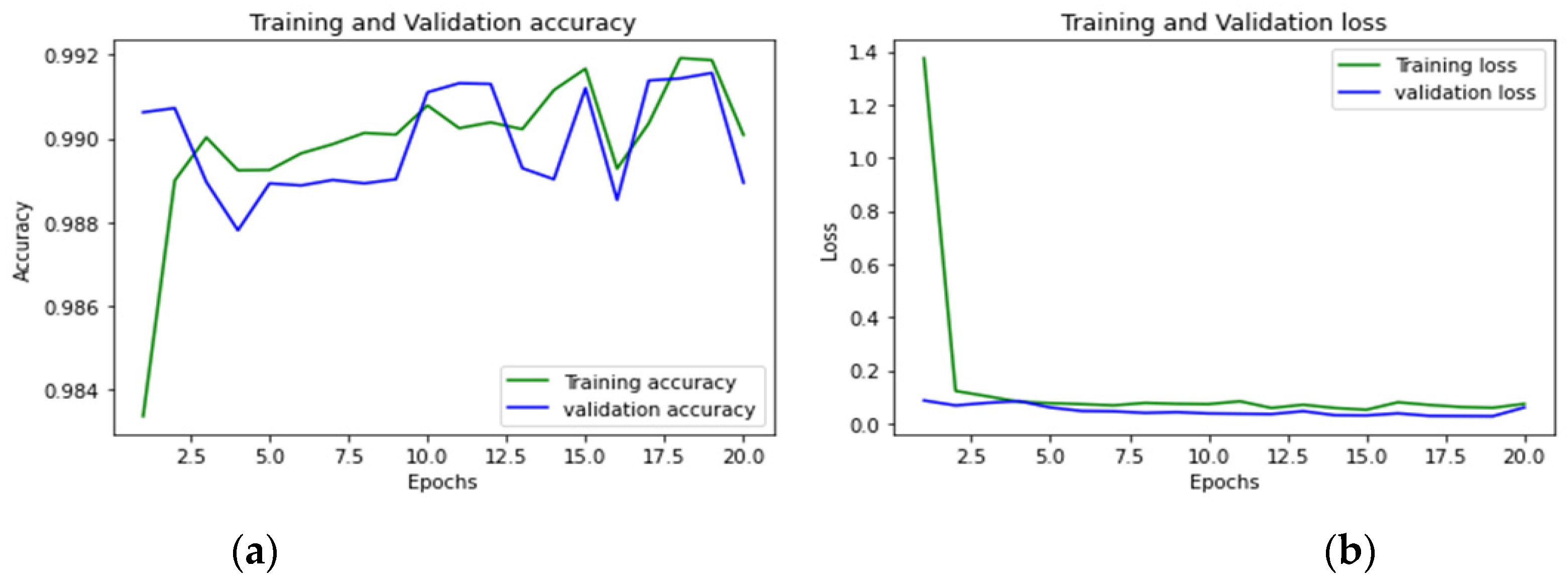
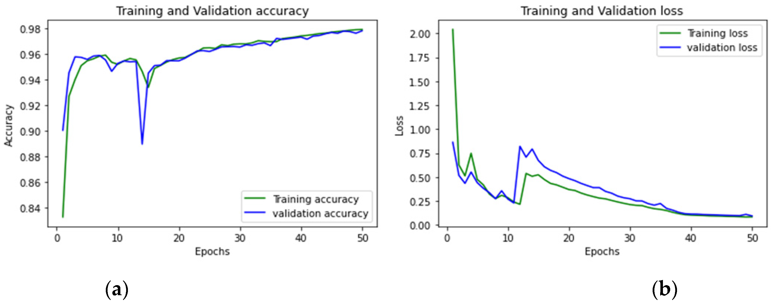
4. Findings and Discussion
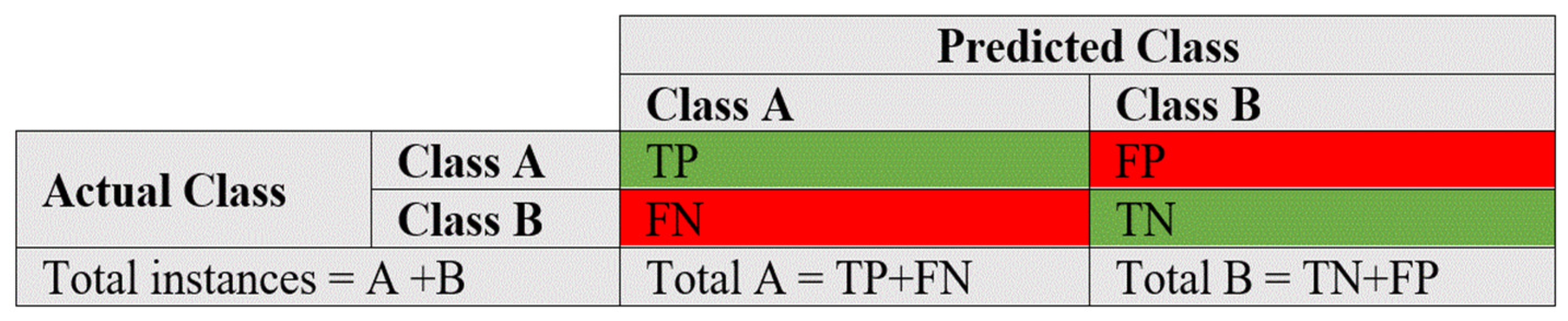
4.1. Evaluation Metrics
4.2. Performance Analysis
5. Conclusions
6. Future Scope
Author Contributions
Funding
Institutional Review Board Statement
Informed Consent Statement
Data Availability Statement
Conflicts of Interest
References
- Prasad, M.; Tripathi, S.; Dahal, K. An efficient feature selection based Bayesian and Rough set approach for intrusion detection. Appl. Soft Comput. J. 2020, 87, 105980. [Google Scholar] [CrossRef]
- Dutt, I.; Borah, S.; Maitra, I.K. Immune System Based Intrusion Detection System (IS-IDS): A Proposed Model. IEEE Access 2020, 8, 34929–34941. [Google Scholar] [CrossRef]
- Khraisat, A.; Gondal, I.; Vamplew, P.; Kamruzzaman, J. Survey of intrusion detection systems: Techniques, datasets and challenges. Cybersecurity 2019, 2, 20. [Google Scholar] [CrossRef]
- Sultana, N.; Chilamkurti, N.; Peng, W.; Alhadad, R. Survey on SDN based network intrusion detection system using machine learning approaches. Peer-to-Peer Netw. Appl. 2018, 12, 493–501. [Google Scholar] [CrossRef]
- Jyothsna, V.; Prasad, V.V.R.; Prasad, K.M. A Review of Anomaly based Intrusion Detection Systems. Int. J. Comput. Appl. 2011, 28, 26–35. [Google Scholar] [CrossRef]
- Vinayakumar, R.; Alazab, M.; Soman, K.P.; Poornachandran, P.; Al-Nemrat, A.; Venkatraman, S. Deep Learning Approach for Intelligent Intrusion Detection System. IEEE Access 2019, 7, 41525–41550. [Google Scholar] [CrossRef]
- Kwon, D.; Kim, H.; Kim, J.; Suh, S.C.; Kim, I.; Kim, K.J. A survey of deep learning-based network anomaly detection. Clust. Comput. 2017, 22, 949–961. [Google Scholar] [CrossRef]
- Fernandez, G.C.; Xu, S. A Case Study on using Deep Learning for Network Intrusion Detection. In Proceedings of the MILCOM 2019—2019 IEEE Military Communications Conference (MILCOM), Norfolk, VA, USA, 12–14 November 2019. [Google Scholar]
- Ring, M.; Wunderlich, S.; Scheuring, D.; Landes, D.; Hotho, A. A survey of network-based intrusion detection data sets. Comput. Secur. 2019, 86, 147–167. [Google Scholar] [CrossRef]
- Magán-Carrión, R.; Urda, D.; Díaz-Cano, I.; Dorronsoro, B. Towards a reliable comparison and evaluation of network intrusion detection systems based on machine learning approaches. Appl. Sci. 2020, 10, 1775. [Google Scholar] [CrossRef]
- Meryem, A.; Ouahidi, B.E.L. Hybrid intrusion detection system using machine learning. Netw. Secur. 2020, 2020, 8–19. [Google Scholar] [CrossRef]
- Abrar, I.; Ayub, Z.; Masoodi, F.; Bamhdi, A.M. A machine learning approach for intrusion detection system on NSL-KDD dataset. In Proceedings of the 2020 International Conference on Smart Electronics and Communication (ICOSEC), Trichy, India, 10–12 September 2020. [Google Scholar]
- Alzahrani, A.O.; Alenazi, M.J. Designing a network intrusion detection system based on machine learning for software defined networks. Future Internet 2021, 13, 111. [Google Scholar] [CrossRef]
- Disha, R.A.; Waheed, S. Performance analysis of machine learning models for intrusion detection system using Gini impurity-based weighted random forest (GIWRF) feature selection technique. Cybersecurity 2022, 5, 1. [Google Scholar] [CrossRef]
- Megantara, A.A.; Ahmad, T. A hybrid machine learning method for increasing the performance of Network Intrusion Detection Systems. J. Big Data 2021, 8, 142. [Google Scholar] [CrossRef]
- De Carvalho Bertoli, G.; Pereira Junior, L.A.; Saotome, O.; Dos Santos, A.L.; Verri, F.A.; Marcondes, C.A.; Barbieri, S.; Rodrigues, M.S.; Parente De Oliveira, J.M. An end-to-end framework for machine learning-based network Intrusion Detection System. IEEE Access 2021, 9, 106790–106805. [Google Scholar] [CrossRef]
- Wang, M.; Zheng, K.; Yang, Y.; Wang, X. An explainable machine learning framework for Intrusion Detection Systems. IEEE Access 2020, 8, 73127–73141. [Google Scholar] [CrossRef]
- Ho, S.; Jufout SAl Dajani, K.; Mozumdar, M. A Novel Intrusion Detection Model for Detecting Known and Innovative Cyberattacks Using Convolutional Neural Network. IEEE Open J Comput Soc. 2021, 2, 14–25. [Google Scholar] [CrossRef]
- Priyanka, V.; Gireesh Kumar, T. Performance Assessment of IDS Based on CICIDS-2017 Dataset. In Information and Communication Technology for Competitive Strategies (ICTCS 2020); Lecture Notes in Networks and Systems; Joshi, A., Mahmud, M., Ragel, R.G., Thakur, N.V., Eds.; Springer: Singapore, 2022; Volume 191. [Google Scholar]
- Sun, P.; Liu, P.; Li, Q.; Liu, C.; Lu, X.; Hao, R.; Chen, J. DL-IDS: Extracting features using CNN-LSTM hybrid network for intrusion detection system. Secur. Commun Netw. 2020, 2020, 8890306. [Google Scholar] [CrossRef]
- Mauro, M.D.; Galatro, G.; Liotta, A. Experimental Review of Neural-based approaches for network intrusion management. IEEE Trans. Netw. Serv. Manag. 2020, 17, 2480–2495. [Google Scholar] [CrossRef]
- Dong, S.; Xia, Y.; Peng, T. Network abnormal traffic detection model based on semi-supervised Deep Reinforcement Learning. IEEE Trans. Netw. Serv. Manag. 2021, 18, 4197–4212. [Google Scholar] [CrossRef]
- Pelletier, C.; Webb, G.I.; Petitjean, F. Deep learning for the classification of sentinel-2 Image time series. In Proceedings of the IGARSS 2019—2019 IEEE International Geoscience and Remote Sensing Symposium, Yokohama, Japan, 28 July–2 August 2019. [Google Scholar]
- Lee, J.; Pak, J.G.; Lee, M. Network intrusion detection system using feature extraction based on deep sparse autoencoder. In Proceedings of the 2020 International Conference on Information and Communication Technology Convergence (ICTC), Jeju, Korea, 21–23 October 2020. [Google Scholar]
- Injadat, M.N.; Moubayed, A.; Nassif, A.B.; Shami, A. Multi-stage optimized machine learning framework for network intrusion detection. IEEE Trans. Netw. Serv. Manag. 2021, 18, 1803–1816. [Google Scholar] [CrossRef]
- Zhu, H.; You, X.; Liu, S. Multiple Ant Colony Optimization Based on Pearson Correlation Coefficient. IEEE Access 2019, 7, 61628–61638. [Google Scholar] [CrossRef]
- Feng, W.; Zhu, Q.; Zhuang, J.; Yu, S. An expert recommendation algorithm based on Pearson correlation coefficient and FP-growth. Clust. Comput. 2018, 22, 7401–7412. [Google Scholar] [CrossRef]
- Shewalkar, A.; Nyavanandi, D.; Ludwig, S.A. Performance Evaluation of Deep Neural Networks Applied to Speech Recognition: RNN, LSTM and GRU. J. Artif. Intell. Soft Comput. Res. 2019, 9, 235–245. [Google Scholar] [CrossRef]
- Xu, C.; Shen, J.; Du, X.; Zhang, F. An Intrusion Detection System Using a Deep Neural Network With Gated Recurrent Units. IEEE Access 2018, 6, 48697–48707. [Google Scholar] [CrossRef]
- Handwritten, I.; Recognition, D. Improved Handwritten Digit Recognition Using Convolutional Neural Networks (CNN). Sensors 2020, 20, 3344. [Google Scholar]
- Acheson, E.; Volpi, M.; Purves, R.S. Machine learning for cross-gazetteer matching of natural features. Int. J. Geogr. Inf. Sci. 2019, 34, 708–734. [Google Scholar] [CrossRef]
- Zhang, Q.; Kong, Q.; Zhang, C.; You, S.; Wei, H.; Sun, R.; Li, L. A new road extraction method using Sentinel-1 SAR images based on the deep fully convolutional neural network. Eur. J. Remote Sens. 2019, 52, 572–582. [Google Scholar] [CrossRef]
- Sheba, K.; Raj, S.G. An approach for automatic lesion detection in mammograms. Cogent Eng. 2018, 5, 1444320. [Google Scholar] [CrossRef]
- Wahlberg, F.; Dahllöf, M.; Mårtensson, L.; Brun, A. Spotting Words in Medieval Manuscripts. Stud. Neophilol. 2014, 86 (Suppl. S1), 171–186. [Google Scholar] [CrossRef]
- Syed, N.F.; Baig, Z.; Ibrahim, A.; Valli, C. Denial of service attack detection through machine learning for the IoT. J. Inf. Telecommun. 2020, 4, 482–503. [Google Scholar] [CrossRef]
- Maseer, Z.K.; Yusof, R.; Bahaman, N.; Mostafa, S.A.; Foozy, C.F.M. Benchmarking of Machine Learning for Anomaly Based Intrusion Detection Systems in the CICIDS2017 Dataset. IEEE Access 2021, 9, 22351–22370. [Google Scholar] [CrossRef]
- Deng, D.; Li, X.; Zhao, M.; Rabie, K.M.; Kharel, R. Deep Learning-Based Secure MIMO Communications with Imperfect CSI for Heterogeneous Networks. Sensors 2020, 20, 1730. [Google Scholar] [CrossRef] [PubMed]
- Gupta, K.; Gupta, D.; Kukreja, V.; Kaushik, V. Fog Computing and Its Security Challenges. In Machine Learning for Edge Computing; CRC Press: Boca Raton, FL, USA, 2022; pp. 1–24. [Google Scholar]
- Ghafir, I.; Hammoudeh, M.; Prenosil, V.; Han, L.; Hegarty, R.; Rabie, K.; Aparicio-Navarro, F.J. Detection of advanced persistent threat using machine-learning correlation analysis. Future Gener. Comput. Syst. 2018, 89, 349–359. [Google Scholar] [CrossRef]
- Garg, H.; Sharma, B.; Shekhar, S.; Agarwal, R. Spoofing detection system for e-health digital twin using EfficientNet Convolution Neural Network. Multimed. Tools Appl. 2022, 81, 26873–26888. [Google Scholar] [CrossRef]
- Datta, P.; Bhardwaj, S.; Panda, S.N.; Tanwar, S.; Badotra, S. Survey of security and privacy issues on biometric system. In Handbook of Computer Networks and Cyber Security; Springer: Cham, Switzerland, 2020; pp. 763–776. [Google Scholar]
- Garg, S.; Singh, R.; Obaidat, M.S.; Bhalla, V.K.; Sharma, B. Statistical vertical reduction-based data abridging technique for big network traffic dataset. Int. J. Commun. Syst. 2020, 33, e4249. [Google Scholar] [CrossRef]


| Reference | Existing Technique | Summary |
|---|---|---|
| Roberto et al., (2020) [10] | NIDS -ML Approaches | Classifier: Logistic regression (LR), SVC-L, SVC-RBF, RF Dataset: UGR’16 Metrics: Precision, Recall, F1, AUC Programming: Python, scikit-optimize |
| Amar et al., (2020) [11] | Hybrid IDS using ML | Classifier: KNN, NB, LR, SVM Dataset: NSL-KDD Metrics: Accuracy, DR, FAR, Precision, Recall, F1 |
| Iram et al., (2020) [12] | An ML Approach for IDS on NSL-KDD Dataset | Classifier: SVM, KNN, LR, NB, MLP, RF, ETC, DT Dataset: NSL-KDD Metrics: Precision, Recall, Accuracy, F1 |
| Abdulsalam et al., (2021) [13] | NIDS Based on Machine Learning for SDNs | Classifier: DT, RF and XGBoost Dataset: NSL-KDD Metrics: Accuracy, DR, ROC, F-score, Precision, Recall |
| Raisa et al., (2022) [14] | IDS using GIWRF feature selection technique | Classifier: DT, GBT, MLP, AdaBoost, LSTM, GRU Dataset: UNSW-NB 15, Network ON_IoT Metrics: Precision, Recall, F1, FPR Programming: Python (Jupyter Notebook) |
| Achmad et al., (2021) [15] | Hybrid ML method for increasing the performance of network IDS | Classifier: Decision Tree Dataset: NSL-KDD, UNSW-NB15 Metrics: Accuracy, sensitivity, specificity, false alarm rate Programming: Python (Jupyter Notebook) |
| Gustavo et al., (2021) [16] | An End-to-End Framework for ML-Based NIDS | Classifier: KNN, RF, XGB, NB, DT, MLP, SVM, and LR Dataset: proposed dataset, MAWILab dataset Metrics: F1, FPR, precision, recall, storage, time, CPU and RAM usage Programming: Python (scikit-learn) |
| Maonan et al., (2020) [17] | An explainable ML Framework for IDS | Classifier: KNN, RF, SVM-RBF, one-vs.-all, and multiclass classifier Dataset: NSL-KDD Metrics: Accuracy, F1, FPR, precision, recall, connections between certain characteristics and attack types Programming: Python (Pytorch) |
| Samson et al., (2021) [18] | Detection of Known, Innovative Cyberattacks Using CNN | Classifier: Convolution Neural Network CNN Dataset: CICIDS 2017 Metrics: TNR, DR, accuracy, FPR |
| Priyanka et al., (2020) [19] | Performance Assessment of IDS-CICIDS-2017 Dataset | Classifier: RF, NB, CNN Dataset: CICIDS2017 (partial) Metrics: Precision, Recall, F1, accuracy Programming: Python (Jupyter Notebook) |
| Sun et al., (2020) [20] | CNN-LSTM hybrid network | Classifier: CNN-LSTM Dataset: CICIDS 2017 Metrics: Accuracy, TPR, FPR, F1 Programming: Python |
| Mario et al., (2020) [21] | Neural-based approaches for Network Intrusion Management | Classifier: ANN Dataset: CICIDS2017/2018 and KDD99 Metrics: Accuracy, f-measure, precision, recall, time complexity Programming: Python |
| Shi et al., (2021) [22] | Semi-Supervised Deep Reinforcement Learning | Classifier: SSDDQN Dataset: NSL-KDD and AWID Metrics: Accuracy, precision, recall, DR, FPR, efficiency Programming: Python |
| Charlotte et al., (2019) [23] | DL for the Classification of Sentinel-2 | Classifier: RF, RNN, CNN Dataset: Sentinel-2 images Metrics: Accuracy, runtime Programming: Python |
| Joohwa et al., (2020) [24] | NIDS using Deep Sparse Autoencoder | Classifier: Single RF, DSAE-RF Dataset: CICIDS 2017 Metrics: Accuracy, precision, F1 Programming: Python |
| Mohammadnoor et al., (2020) [25] | Multi-Stage Optimized ML for NIDS | Classifier: KNN, RF Dataset: CICIDS 2017 and the UNSW-NB 2015 Metrics: Accuracy, precision, recall, FAR Programming: Python |
| Sub-Dataset | Attacks |
|---|---|
| Tuesday Samples | benign ftpPatatorAttack sshPatatorAttack |
| Wed. Samples | benign goldeneyeAttack hulkAttack slowhttptestAttack slowlorisAttack heartbleedAttack |
| Thur. Morning Samples | benign bruteForceAttack SqlInjectionAttack XSSAttack |
| Thurs. Afternoon Samples | benign infiltrationAttack |
| Fri. Morning Samples | benign botAttack |
| Fri. Afternoon Samples-DDoS | benign ddosAttack |
| Friday Afternoon Samples-PortScan | benign portscanAttack |
| Sub-Dataset | Number of Instances | |
|---|---|---|
| With Redundancy | Without Redundancy | |
| Tuesday_BruteForce | 445,909 | 425,240 |
| Wednesday_DoS/DDoS | 692,703 | 613,287 |
| Thurs_Morning_WebAttacks | 170,366 | 164,300 |
| Thurs. Afternoon_Infiltration | 288,602 | 254,625 |
| Fri. Morning_Bot | 191,033 | 184,145 |
| Fri. Afternoon-DDoS | 225,745 | 223,666 |
| Fri. Afternoon-PortScan | 286,467 | 214,114 |
| Sub-Dataset | Total Features | Selected Features |
|---|---|---|
| BruteForce | 77 | 43 |
| DoS/DDoS | 77 | 41 |
| WebAttacks | 77 | 39 |
| Infiltration | 77 | 40 |
| Bot | 77 | 37 |
| DDoS | 77 | 39 |
| PortScan | 77 | 37 |
| Parameter | 1 | 2 | 3 | 4 | 5 | 6 |
|---|---|---|---|---|---|---|
| Type | C | C | C | G | G | H |
| No. of neurons | 32 | 32 | 32 | 64 | 64 | No. of classes |
| Filter Size | (1) | (1) | (1) | (1) | (1) | (1) |
| Activation Fun. | ReLU | ReLU | ReLU | ReLU | ReLU | Smax |
| Parameters | BENIGN | FTPPatator | SSHPatator |
|---|---|---|---|
| Precision | 0.9984 | 0.9788 | 0.9847 |
| Recall | 1.00 | 0.98 | 0.86 |
| TN | 2919 | 138,292 | 139,184 |
| FP | 208 | 42 | 15 |
| TP | 137,150 | 1947 | 968 |
| FN | 53 | 49 | 163 |
| FPR | 0.0665 | 0.0003 | 0.0001 |
| TPR | 0.9996 | 0.9754 | 0.8558 |
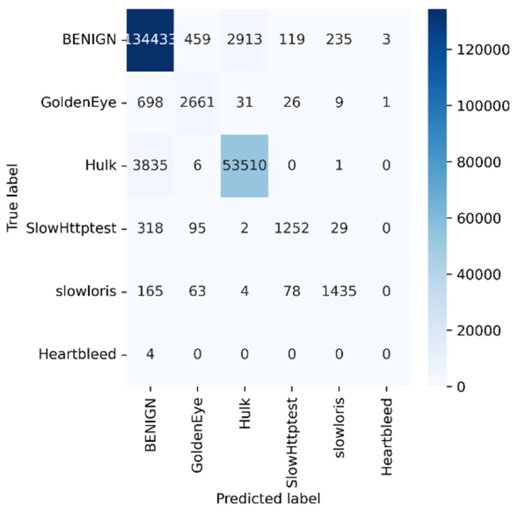
| Parameters | BENIGN | Goldeneye | Hulk | Slowhttptest | Slowloris | Heartbleed |
|---|---|---|---|---|---|---|
| Precision | 0.9640 | 0.8102 | 0.9477 | 0.8488 | 0.8396 | 0 |
| Recall | 0.97 | 0.78 | 0.93 | 0.74 | 0.82 | 0 |
| TN | 59,203 | 198,336 | 142,083 | 200,466 | 200,366 | 202,377 |
| FP | 5020 | 623 | 2950 | 223 | 274 | 4 |
| TP | 134,433 | 2661 | 53,510 | 1252 | 1435 | 0 |
| FN | 3729 | 765 | 3842 | 444 | 310 | 4 |
| FPR | 0.078 | 0.003 | 0.020 | 0.001 | 0.001 | 0 |
| TPR | 0.9730 | 0.7767 | 0.9330 | 0.7382 | 0.8223 | 0 |
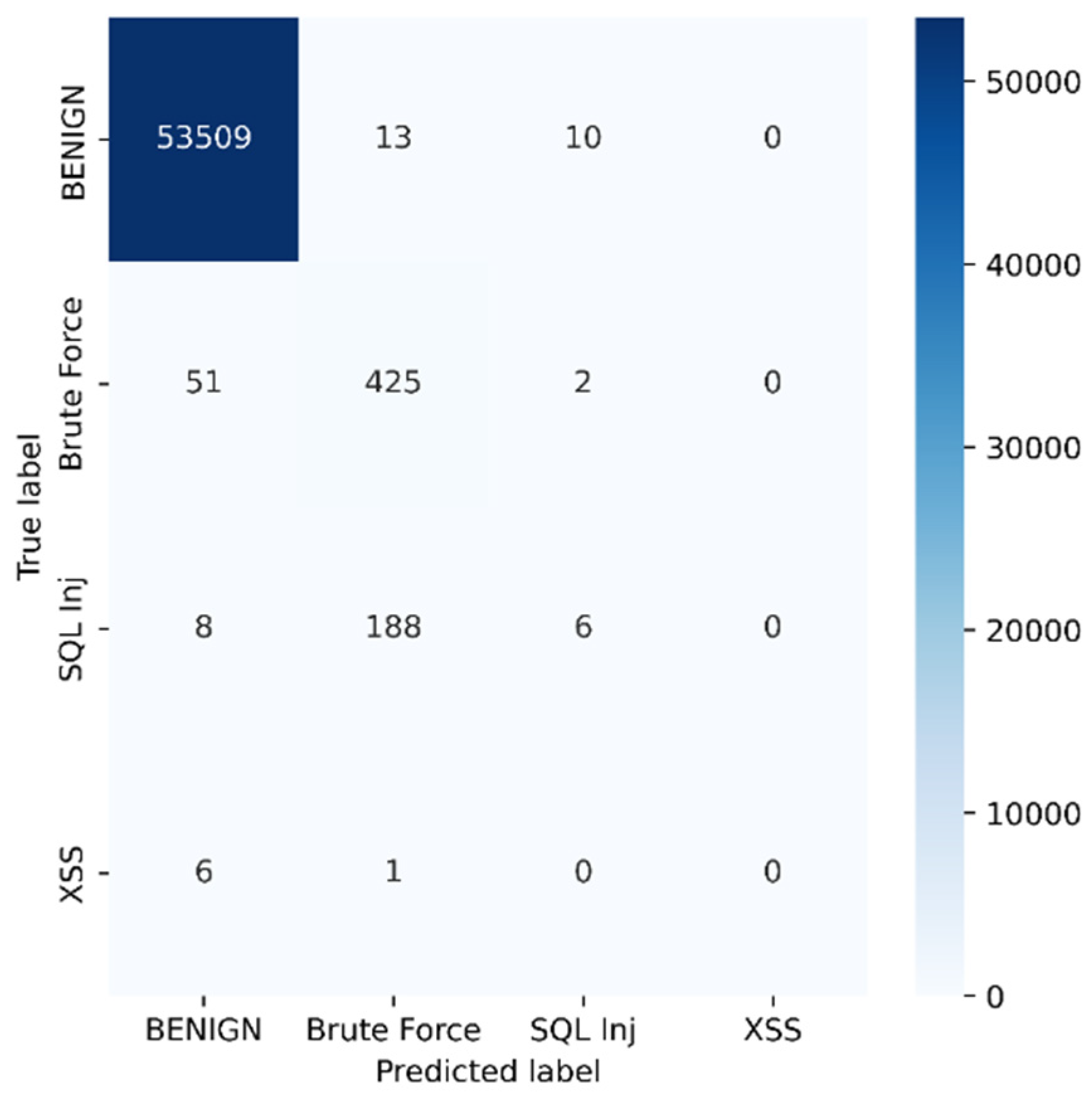
| Parameters | BENIGN | Brute Force | Sql Inj | XSS |
|---|---|---|---|---|
| Precision | 0.9987 | 0.6778 | 0.3333 | 0 |
| Recall | 1.00 | 0.89 | 0.03 | 0.00 |
| TN | 622 | 53,539 | 54,005 | 54,212 |
| FP | 65 | 202 | 12 | 0 |
| TP | 53,509 | 425 | 6 | 0 |
| FN | 23 | 53 | 196 | 7 |
| FPR | 0.0946 | 0.0037 | 0.0002 | 0 |
| TPR | 0.9995 | 0.8891 | 0.0297 | 0 |
| Parameters | BENIGN | Infiltration |
|---|---|---|
| Precision | 0.9999 | 0.0312 |
| Recall | 1.00 | 0.14 |
| TN | 1 | 83,989 |
| FP | 6 | 31 |
| TP | 83,989 | 1 |
| FN | 31 | 6 |
| FPR | 0.8571 | 0.0003 |
| TPR | 0.9996 | 0.1428 |
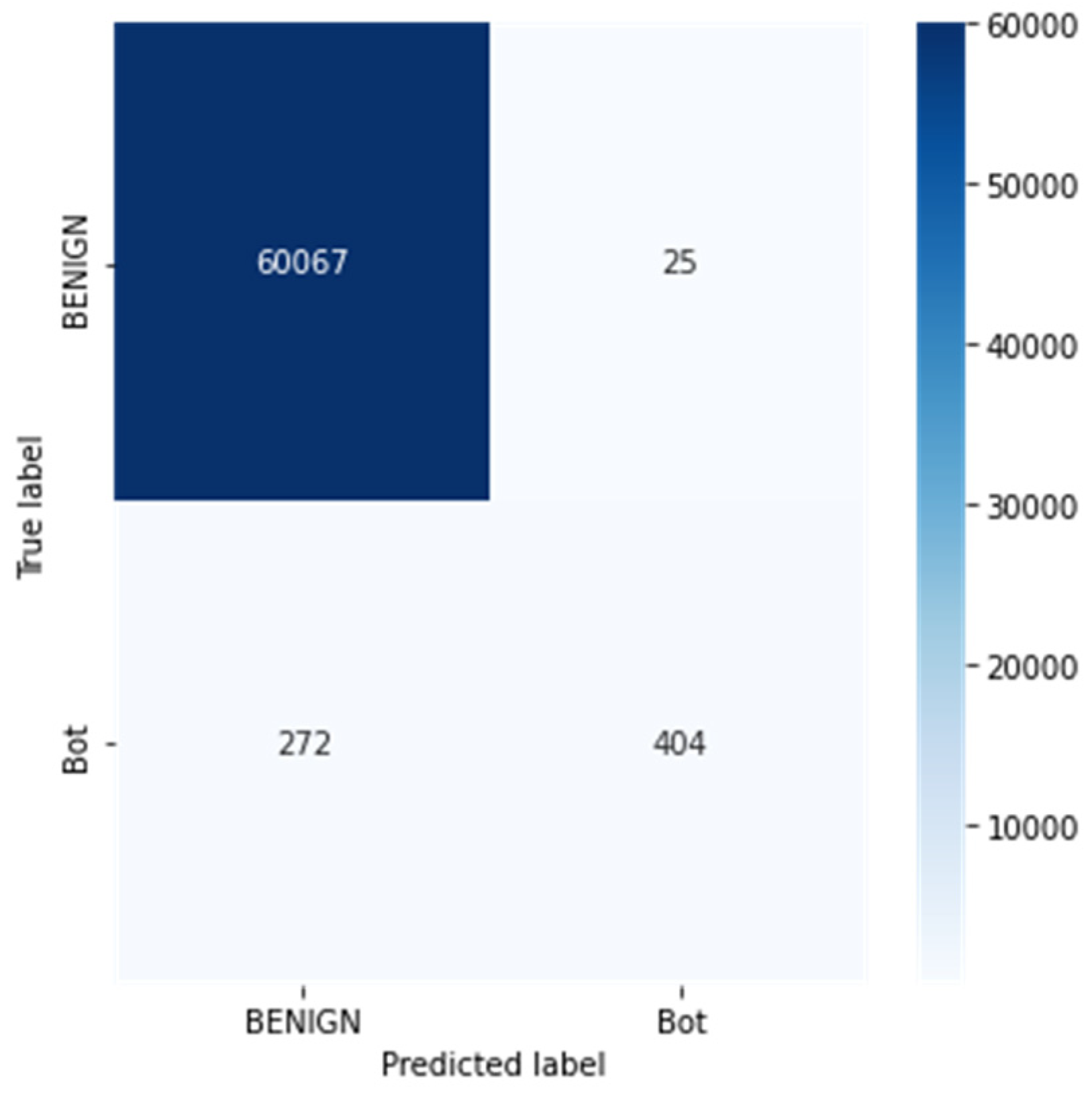
| Parameters | BENIGN | Bot |
|---|---|---|
| Precision | 0.9954 | 0.9417 |
| Recall | 1.00 | 0.60 |
| TN | 404 | 60,067 |
| FP | 272 | 25 |
| TP | 60,067 | 404 |
| FN | 25 | 272 |
| FPR | 0.4023 | 0.0004 |
| TPR | 0.9995 | 0.5976 |
| Parameters | BENIGN | DDoS |
|---|---|---|
| Precision | 0.9902 | 0.9699 |
| Recall | 0.96 | 0.99 |
| TN | 42,041 | 30,170 |
| FP | 297 | 1302 |
| TP | 30,170 | 42,041 |
| FN | 1302 | 297 |
| FPR | 0.0070 | 0.0413 |
| TPR | 0.9586 | 0.9929 |
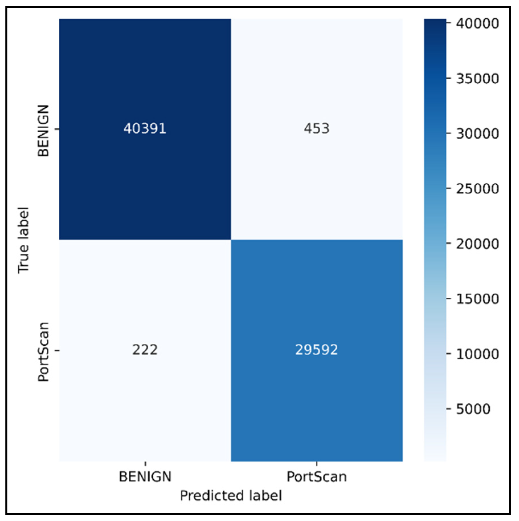
| Parameters | BENIGN | PortScan |
|---|---|---|
| Precision | 0.9945 | 0.9849 |
| Recall | 0.99 | 0.99 |
| TN | 29,592 | 40,391 |
| FP | 222 | 453 |
| TP | 40,391 | 29,592 |
| FN | 453 | 222 |
| FPR | 0.0074 | 0.0110 |
| TPR | 0.9889 | 0.9925 |
| Sub-Dataset | Accuracy |
|---|---|
| BruteForce | 99.81% |
| DoS/DDoS | 95.50% |
| WebAttacks | 99.48% |
| Infiltration | 99.95% |
| Bot | 99.51% |
| DDoS | 97.83% |
| PortScan | 99.04% |
| Model | No. of Attributes | Accuracy |
|---|---|---|
| Proposed CNN–GRU | Less than 44 | 98.73% |
| CNN [18] | 77 | 94.96% |
| CNN [19] | 77 | 99.7% |
| CNN-LSTM [20] | 77 | 98.67% |
| CNN [36] | 77 | 99.47% |
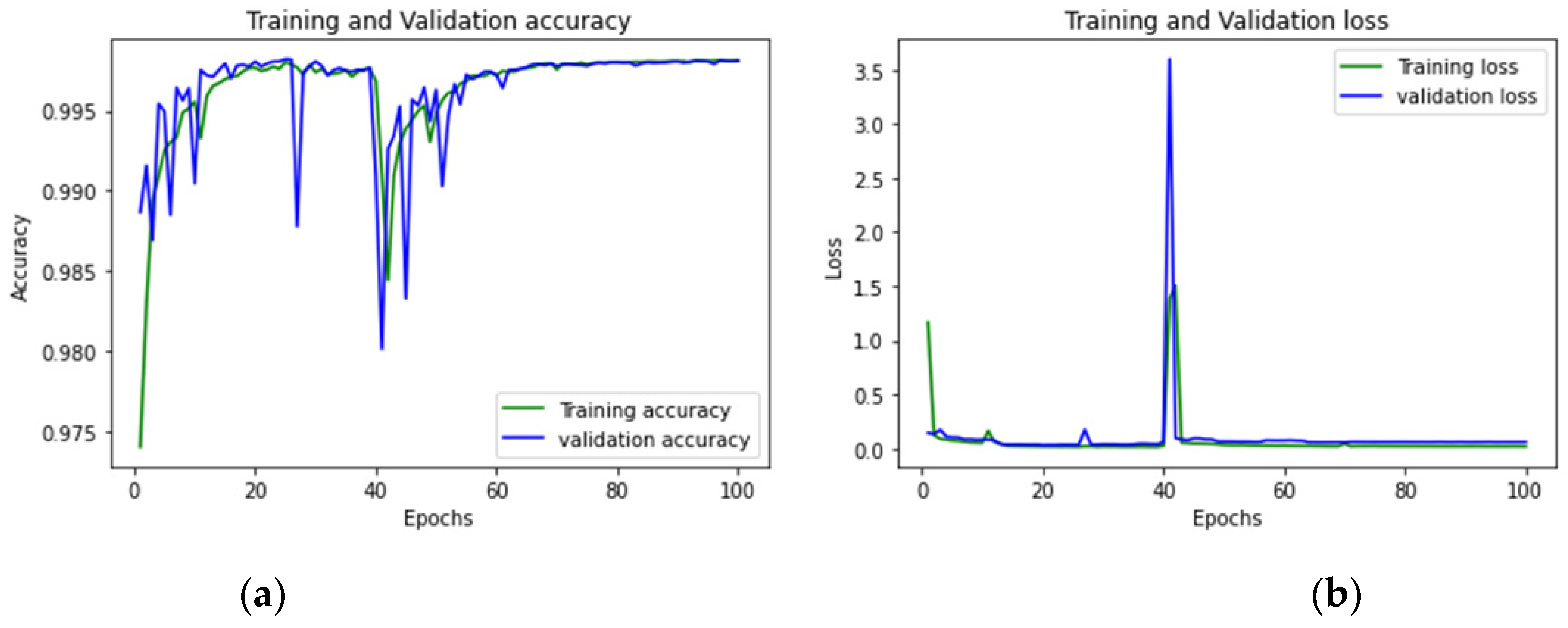
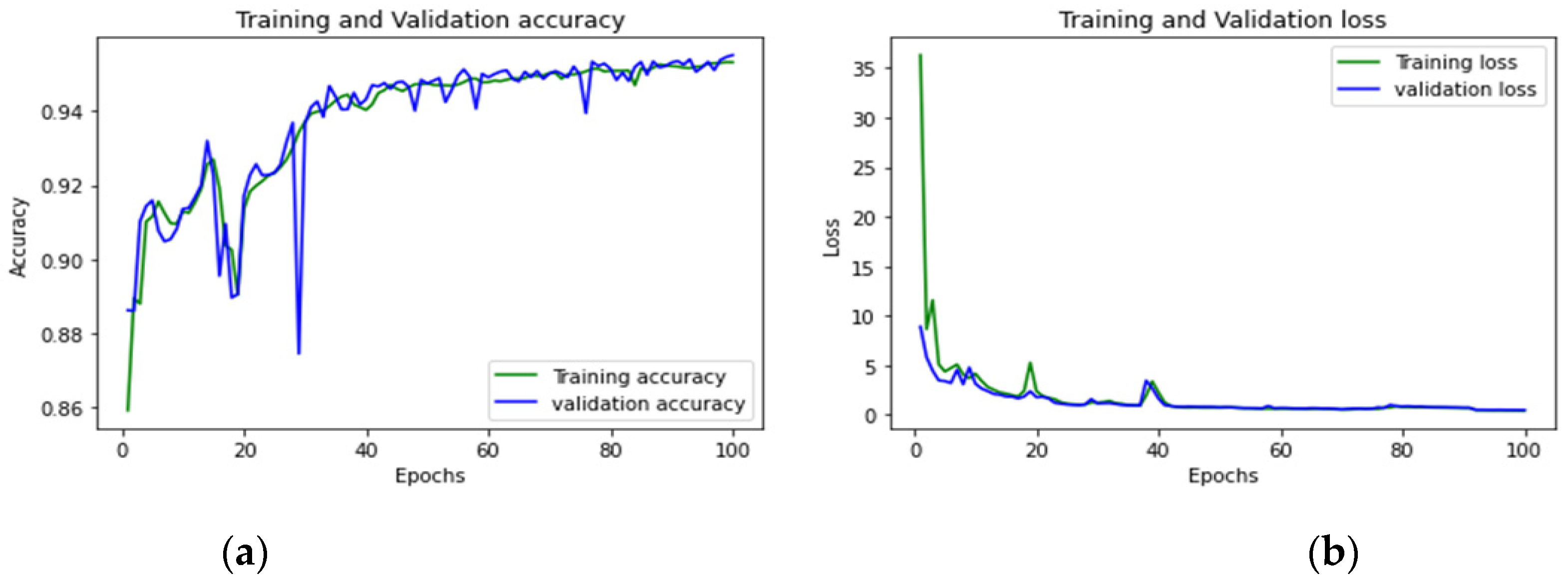
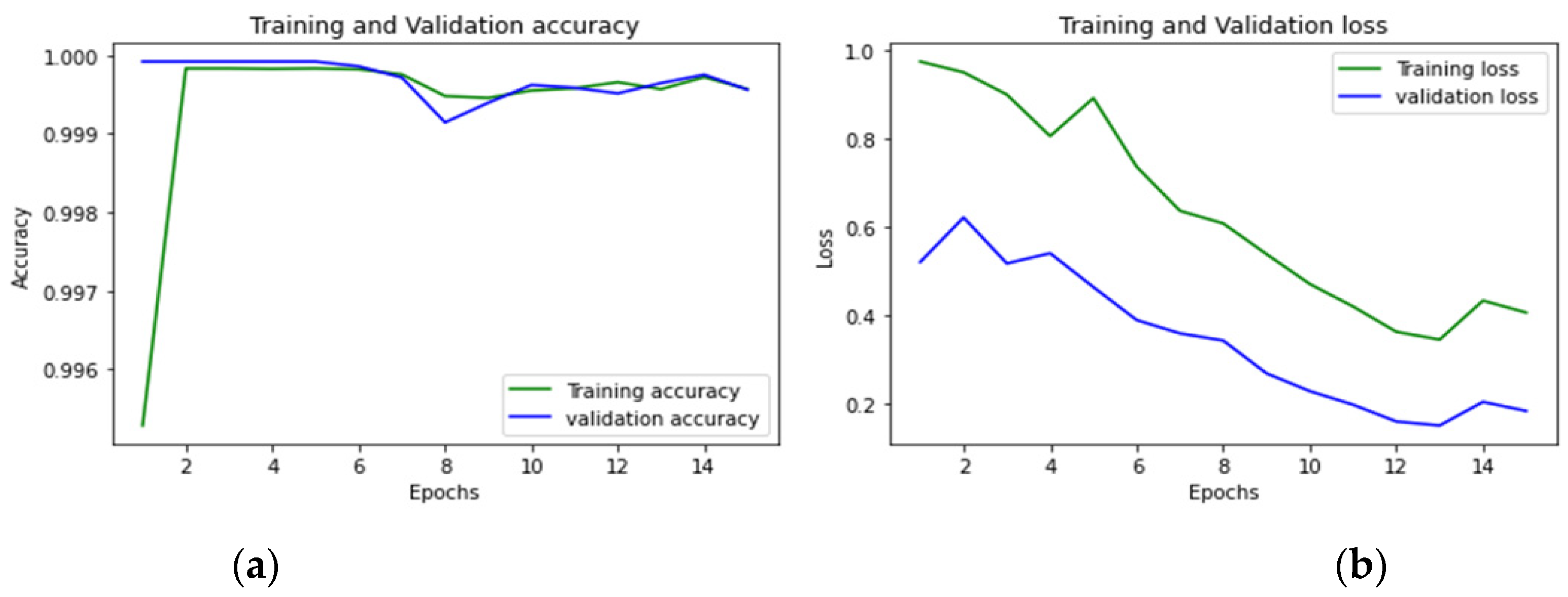
| Sub-Dataset | Epochs |
|---|---|
| BruteForce | 100 |
| DoS/DDoS | 100 |
| WebAttacks | 100 |
| Infiltration | 15 |
| Bot | 20 |
| DDoS | 50 |
| PortScan | 20 |
Disclaimer/Publisher’s Note: The statements, opinions and data contained in all publications are solely those of the individual author(s) and contributor(s) and not of MDPI and/or the editor(s). MDPI and/or the editor(s) disclaim responsibility for any injury to people or property resulting from any ideas, methods, instructions or products referred to in the content. |
© 2023 by the authors. Licensee MDPI, Basel, Switzerland. This article is an open access article distributed under the terms and conditions of the Creative Commons Attribution (CC BY) license (https://creativecommons.org/licenses/by/4.0/).
Share and Cite
Henry, A.; Gautam, S.; Khanna, S.; Rabie, K.; Shongwe, T.; Bhattacharya, P.; Sharma, B.; Chowdhury, S. Composition of Hybrid Deep Learning Model and Feature Optimization for Intrusion Detection System. Sensors 2023, 23, 890. https://doi.org/10.3390/s23020890
Henry A, Gautam S, Khanna S, Rabie K, Shongwe T, Bhattacharya P, Sharma B, Chowdhury S. Composition of Hybrid Deep Learning Model and Feature Optimization for Intrusion Detection System. Sensors. 2023; 23(2):890. https://doi.org/10.3390/s23020890
Chicago/Turabian StyleHenry, Azriel, Sunil Gautam, Samrat Khanna, Khaled Rabie, Thokozani Shongwe, Pronaya Bhattacharya, Bhisham Sharma, and Subrata Chowdhury. 2023. "Composition of Hybrid Deep Learning Model and Feature Optimization for Intrusion Detection System" Sensors 23, no. 2: 890. https://doi.org/10.3390/s23020890
APA StyleHenry, A., Gautam, S., Khanna, S., Rabie, K., Shongwe, T., Bhattacharya, P., Sharma, B., & Chowdhury, S. (2023). Composition of Hybrid Deep Learning Model and Feature Optimization for Intrusion Detection System. Sensors, 23(2), 890. https://doi.org/10.3390/s23020890