Target Localization in Wireless Sensor Networks Based on Received Signal Strength and Convex Relaxation

Abstract

A new positioning algorithm based on RSS measurement is proposed. The algorithm adopts maximum likelihood estimation and semi-definite programming. The received signal strength model is transformed to a non-convex estimator for the positioning of the target using the maximum likelihood estimation. The non-convex estimator is then transformed into a convex estimator by semi-definite programming, and the global minimum of the target location estimation is obtained. This algorithm aims at the $L_0$ known problem and then extends its application to the case of $L_0$ unknown. The simulations and experimental results show that the proposed algorithm has better accuracy than the existing positioning algorithms.

1. Introduction

With the development of wireless sensor networks (WSNs) [1,2,3,4,5,6,7,8,9,10,11,12,13], the Internet of things has become common. Positioning algorithms are widely used in intelligent warehouse, robot cooperation, instrument navigation, position monitoring, etc. The predefined points are known as the anchors, while the target refers to the point whose position needs to be estimated. The common measurements are angle of arrival (AOA) [14,15,16,17], time of arrival (TOA) [18,19,20], time difference of arrival (TDOA) [21,22] and received signal strength (RSS) [23,24,25,26,27,28,29]. However, AOA requires antenna arrays. TOA and TDOA require clock synchronization, which greatly increases the costs. Compared with other measurements, the RSS measurement is easier and a lower cost to obtain. Hence, we focus on it in this paper. There are two models of RSS: one is based on signal strength, and the other is on path loss. This paper adopts the latter.

Among the existing RSS positioning algorithms, a common approach is to construct a non-convex function about the target and then find the extreme value of the function using some mathematical algorithms, such as gradient descent, coordinate descent, genetic algorithm, and golden section algorithm. However, because of the noise in the received signal, the extremum of the non-convex equation may not be the global optimal solution, but the local optimum instead. Therefore, a more accepted approach is using convex optimization schemes to get a convex equation, and then find the global optimal value. The least squares (LS), least relative error (LSRE) and weighted least squares (WLS) are applied in most optimization problems. In the literature, Robin, WO. [30], Tomic, S. [31], Wang, Z. [32], Surya, VP. [33] and Mei, X. [34], all choose to ignore the difference of the standard deviation of noise after the Taylor expansion of the term containing the amount of noise in the model transformation. Therefore, if the received signal strength contains noise, the final estimated position has some deviation, which increases as the noise standard deviation increases, and the deviation also increases, resulting in the poor estimation accuracy. The SOCP1 method proposed by Tomic, S. [35] and the SDP1 method proposed by Chang, S. [36] used the convex optimization to solve this problem. They also considered cooperative scenes. Coluccia, A. proposed a Bayesian formulation of the ranging problem [37]. This method is called “optimal ML range-free”. The DEOR method [38] and DEOR-fast method [39] proposed by Najarro, L.A.C. employed the three techniques of DE, OBL and adaptive redirection. These two methods achieved good accuracy, but the lower and upper bounds for the initial population is hard to be sure about. This paper proposes a new positioning algorithm based on maximum likelihood estimation and semi-definite programming (“MLE-SDP”), which takes into account the variation of noise standard deviation. The basic steps of this algorithm is to transform the path loss model of the received signal into a relatively simple expression without a logarithm and expand the term with noise by Taylor series to obtain a new noise term. The variance of the new term is proportional to the distance between the target and each anchor. Then, the maximum likelihood estimation function is constructed, and a non-convex estimator is obtained. Next, we use semi-definite programming [40] to transform the non-convex variables and obtain a constrained convex estimate. The estimator of the target can be obtained by solving the convex problem.

The main contributions of this paper is as follows:

• The RSS model is transformed into a pseudo-linear system with new noise;
• Based on LS criterion, a new non-convex objective function is derived to solve the target positioning problem;
• The non-convex objective function is transformed into a convex objective function by semi-definite programming.

The experiments were carried to verify the performance of the proposed algorithm. It is compared with three existing common algorithms and the Cramer–Rao lower bound (CRLB). The simulation results show that the proposed algorithm achieves substantial improvements in accuracy, at the same complexity and running time. The results of field test are also given in Section 5.

2. System Model and Problem Formulation

Suppose a two-dimensional (or three-dimensional) sensor network is composed of N anchors and a target with unknown position. The positions of the target and the i-th anchor are represented by $\mathbf{x}$ and ${\mathbf{s}}_i$ ($i=1,\dots ,N$), respectively. As show in Figure 1, $d_i$ represent the distance between the i-th anchor and the target. Assuming that the received signal noise follows the normal distribution $n_i\sim N\left(0,{\sigma }_{n_i}^2\right)$. That means the mean of $n_i$ is zero and the standard deviation is ${\sigma }_{n_i}$, making the system model to be

$$\begin{array}{c}\hfill L_i=L_0+10\gamma {log}_{10}\frac{∥\mathbf{x}-{\mathbf{s}}_i∥}{d_0}+n_i,i=1,\dots ,N\end{array}$$

(1)

where $L_i$ is the RSS measurement received by the i-th anchor, and $L_0$ is the RSS measurement received by the anchor. When the distance between the anchor and the target is $d_0$, $d_0$ is the reference distance, usually set as 1 m. $\gamma$ is the path loss index, and it is generally between 2.2 and 4. This paper takes 2.2 because this paper is based on LOS scenes. $n_i$ is the received signal noise of the i-th measurement. When $L_0$ is known, the maximum likelihood estimation is used as

$$\begin{array}{c}\hfill \underset{\mathbf{x}}{min}\sum _{i=1}^N\frac{{(L_i-L_0-10\gamma {log}_{10}\frac{∥\mathbf{x}-{\mathbf{s}}_i∥}{d_0})}^2}{{{\sigma }_{n_i}}^2},i=1,\dots ,N.\end{array}$$

(2)

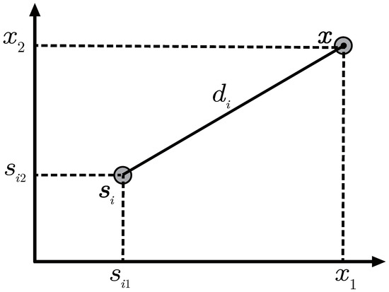
Figure 1. Schematic diagram of anchor and target position.

When $L_0$ is unknown, the maximum likelihood estimation is used as

$$\begin{array}{c}\hfill \underset{\mathbf{x},L_0}{min}\sum _{i=1}^N\frac{{(L_i-L_0-10\gamma {log}_{10}\frac{∥\mathbf{x}-{\mathbf{s}}_i∥}{d_0})}^2}{{{\sigma }_{n_i}}^2},i=1,\dots ,N.\end{array}$$

(3)

Because large-scale examples of these problems cannot be solved by accurate algorithm, Equations (2) and (3) are NP-hard problems which are very complex non-convex estimators, and it is difficult to find the global optimal solution.

3. The Proposed Algorithm

In this section, we introduce the estimator of the target position based on the maximum likelihood estimation in the two-dimensional case and use semi-definite programming to change the non-convex estimator into convex, so that we can find the global optimal solution. For 3D, it is similar to 2D.

In Section 3.1, $L_0$ is known, and in Section 3.2, $L_0$ is unknown. Table 1 lists the symbols that appear frequently in this section.

Table 1. Symbols and notations.

Symbol	Explanation
$L_i$	The RSS measurements
$d_0$	The reference distance
$L_0$	The RSS measurements when $d_0=1$
$\gamma$	The pass-loss exponent
$\mathbf{x}$	The position of the target node
${\mathbf{s}}_i$	The position of the i-th anchor node
N	The number of anchor nodes
$d_i$	The range between the target node and the i-th anchor node
$n_i$	The measurement noise between the target node and the i-th anchor node
$\sigma$	The standard deviation of measurement noises

3.1. $L_0$ Known Positioning Algorithm

To simplify the system model, subtracting $L_0$ from both sides of Equation (1) and dividing by $10\gamma$, and taking the power of 10 at the same time, we obtain

$$\begin{array}{c}\hfill d_0{10}^{\frac{L_i-L_0}{10\gamma }}=∥\mathbf{x}-{\mathbf{s}}_i∥{10}^{\frac{n_i}{10\gamma }},i=1,\dots ,N.\end{array}$$

(4)

Let us expand ${10}^{\frac{n_i}{10\gamma }}$ by McLaughlin, just ${10}^{\frac{n_i}{10\gamma }}\approx 1+\frac{ln10}{10\gamma }{n}_i$, and we obtain

$$\begin{array}{c}\hfill {\alpha }_i\eta =∥\mathbf{x}-{\mathbf{s}}_i∥+\frac{ln10}{10\gamma }∥\mathbf{x}-{\mathbf{s}}_i∥n_i,i=1,\dots ,N\end{array}$$

(5)

where ${\alpha }_i=d_0{10}^{\frac{L_i}{10\gamma }}$, $\eta ={10}^{-\frac{L_0}{10\gamma }}$. According to ${\alpha }_i\eta \approx ∥\mathbf{x}-{\mathbf{s}}_i∥$, we obtain

$$\begin{array}{c}\hfill {\alpha }_i\eta =∥\mathbf{x}-{\mathbf{s}}_i∥+{\xi }_i,i=1,\dots ,N\end{array}$$

(6)

where ${\xi }_i=\frac{ln10}{10\gamma }{\alpha }_i\eta n_i$, a new noise ${\xi }_i$ with mean square error $\frac{ln10}{10\gamma }{\alpha }_i\eta \sigma$ is obtained, a non-convex equation is constructed according to maximum likelihood estimation as

$$\begin{array}{c}\hfill \underset{\mathbf{x}}{min}\underset{i=1}{\sum ^N}\frac{{\left({\alpha }_i\eta -∥\mathbf{x}-{\mathbf{s}}_i∥\right)}^2}{{\left(\frac{ln10}{10\gamma }{\alpha }_i\eta \sigma \right)}^2}\end{array}$$

(7)

because $\frac{ln10}{10\gamma }$, $\eta$, $\sigma$ are constant, they are not affected when estimating $\mathbf{x}$. Thus, they can be removed, an unfolding molecule, and we obtain

$$\begin{array}{c}\hfill \underset{\mathbf{x}}{min}\underset{i=1}{\sum ^N}\frac{{∥\mathbf{x}-{\mathbf{s}}_i∥}^2-2{\alpha }_i\eta ∥\mathbf{x}-{\mathbf{s}}_i∥}{{{\alpha }_i}^2}+1\end{array}$$

(8)

The addition of 1 in the objective function does not affect the estimated value $\mathbf{x}$. Thus, Equation (8) can be written as

$$\begin{array}{c}\hfill \underset{x,d,r}{min}\underset{i=1}{\sum ^N}\frac{r_i-2{\alpha }_i\eta d_i}{{{\alpha }_i}^2}\end{array}$$

(9a)

$$\begin{array}{c}\hfill s.t.d_i=∥\mathbf{x}-{\mathbf{s}}_i∥\end{array}$$

(9b)

$$\begin{array}{c}\hfill r_i={d_i}^2\end{array}$$

(9c)

where $d_i=∥\mathbf{x}-{\mathbf{s}}_i∥$, $r_i={d_i}^2$. Now, the objective function is transformed into convex, and then the constraints are transformed as

$$\begin{array}{c}\hfill \underset{\mathbf{x},y,d,r}{min}\underset{i=1}{\sum ^N}\frac{r_i-2{\alpha }_i\eta d_i}{{{\alpha }_i}^2}\end{array}$$

(10a)

$$\begin{array}{c}\hfill s.t.r_i=y-2{{\mathbf{s}}_i}^T\mathbf{x}+{{\mathbf{s}}_i}^T{\mathbf{s}}_i\end{array}$$

(10b)

$$\begin{array}{c}\hfill y={\mathbf{x}}^T\mathbf{x}\end{array}$$

(10c)

$$\begin{array}{c}\hfill r_i={d_i}^2.\end{array}$$

(10d)

Using semi-definite programming, we transform Equation (10) into convex and obtain the final estimator as

$$\begin{array}{c}\hfill \underset{\mathbf{x},y,d,r}{min}\underset{i=1}{\sum ^N}\frac{r_i-2{\alpha }_i\eta d_i}{{{\alpha }_i}^2}\end{array}$$

(11a)

$$\begin{array}{c}\hfill s.t.r_i=y-2{{\mathbf{s}}_i}^T\mathbf{x}+{{\mathbf{s}}_i}^T{\mathbf{s}}_i\end{array}$$

(11b)

$$\begin{array}{c}\hfill \left[\begin{array}{cc}{\mathbf{x}}^T& y\\ {\mathbf{I}}_2& \mathbf{x}\end{array}\right]\ge 0\end{array}$$

(11c)

$$\begin{array}{c}\hfill \left[\begin{array}{cc}{d}_i& r_i\\ 1& d_i.\end{array}\right]\ge 0\end{array}$$

(11d)

The estimator Equation (11) is a new positioning algorithm when $L_0$ is known, and it is called “MLE-SDP”.

For Equation (10), the form of second-order cone programming can also be used, and the transformed estimator Equation (12) is called “MLE-SOCP” as

$$\begin{array}{cc}\hfill & \underset{\mathbf{x},y,d,r}{min}\underset{i=1}{\sum ^N}\frac{r_i-2{\alpha }_i\eta d_i}{{{\alpha }_i}^2}\hfill \end{array}$$

(12a)

$$\begin{array}{cc}\hfill s.t.r_i& =y-2{{\mathbf{s}}_i}^T\mathbf{x}+{{\mathbf{s}}_i}^T{\mathbf{s}}_i\hfill \end{array}$$

(12b)

$$\begin{array}{cc}\hfill & ∥\left[\begin{array}{c}2\mathbf{x}\\ 1-y\end{array}\right]∥\le 1+y\hfill \end{array}$$

(12c)

$$\begin{array}{cc}\hfill & ∥\left[\begin{array}{c}2d_i\\ 1-r_i.\end{array}\right]∥\le 1+r_i\hfill \end{array}$$

(12d)

Because the simulation results of the “MLE-SDP” algorithm are better than the “MLE-SOCP” algorithm’s, this paper only uses the “MLE-SDP” algorithm to compare with other algorithms.

3.2. $L_0$ Unknown Positioning Algorithm

Because the transformation of $L_0$ unknown case is very similar to $L_0$ known case, the final estimator is given directly as

$$\begin{array}{c}\hfill \underset{\mathbf{x},y,d,r,\eta ,u}{min}\underset{i=1}{\sum ^N}\frac{r_i-2{\alpha }_i{u}_i}{{{\alpha }_i}^2}\end{array}$$

(13a)

$$\begin{array}{c}\hfill s.t.r_i=y-2{{\mathbf{s}}_i}^T\mathbf{x}+{{\mathbf{s}}_i}^T{\mathbf{s}}_i\end{array}$$

(13b)

$$\begin{array}{c}\hfill \left[\begin{array}{cc}{\mathbf{x}}^T& y\\ {\mathbf{I}}_2& \mathbf{x}\end{array}\right]\ge 0\end{array}$$

(13c)

$$\begin{array}{c}\hfill \left[\begin{array}{cc}{d}_i& r_i\\ 1& d_i\end{array}\right]\ge 0\end{array}$$

(13d)

$$\begin{array}{c}\hfill \left[\begin{array}{cc}\eta & u_i\\ 1& d_i\end{array}\right]\ge 0\end{array}$$

(13e)

the estimator Equation (13) is the positioning algorithm, when $L_0$ is unknown, called “MLE-SDP2” in this paper.

4. Simulation Results

In this section, the performance of the proposed algorithms “MLE-SDP” and “MLE-SDP2” are verified by MATLAB simulations. In Section 4.1, the “MLE-SDP” algorithm is compared with the “LS-SDP” algorithm, the “LS-SOCP” algorithm, the “LSRE-SOCP” algorithm, the “optimal ML range-free” algorithm, the “SOCP1” algorithm, the “DEOR1” algorithm and the “DEOR-fast1” algorithm. In Section 4.2, the “MLE-SDP2” algorithm is compared with the “LS-SDP2” algorithm, the “LS-SOCP2” algorithm, the “SOCP2” method, the “DEOR2” method and the “DEOR-fast2” method. In addition, the Cramer–Rao lower bound (CRLB) is also provided in both conditions. CRLB is the best effect that can estimate parameters by using the existing information. The closer to CRLB, the better the performance of the algorithm.

All RSS measurements are generated by Equation (1). The measurement noise is based on normal distribution. Anchors are randomly generated in a square area with a side length of 100 m. In order to avoid the influence of the special distribution of anchors, the position of anchors is reset in each simulation. The settings of reference distance, path loss, reference measured value, simulation times and other variables are given in Table 2. The root mean square error (RMSE) is used to evaluate the performance of the algorithm. The definition of RMSE is $\sqrt{\frac{1}{M_c}{\displaystyle \sum _{i=1}^{Mc}}{∥{\mathbf{x}}_i-{\widehat{\mathbf{x}}}_i∥}^2}$, where ${\mathbf{x}}_i$ is the position of the target, ${\widehat{\mathbf{x}}}_i$ is the estimated position of the target and $Mc$ is the simulation times.

Table 2. Simulation parameter settings.

Symbol	Describe	Value
$d_0$	reference distance	1 m
$\gamma$	path loss	4
$L_0$	reference measured value	−10 dBm
$Mc$	simulation times	5000

The variables of ${\sigma }_{n_i}$ and N are given in Table 3.

Table 3. Variables in Figure 2, Figure 3, Figure 4, Figure 5, Figure 6 and Figure 7.

	${\mathit{\sigma }}_{{\mathit{n}}_{\mathit{i}}}$	N
Figure 2	1–6 dBm	9
Figure 3	4 dBm	6–16
Figure 4	4 dBm	9
Figure 5	1–6 dBm	9
Figure 6	4 dBm	6–16
Figure 7	4 dBm	9

4.1. $L_0$ Is Known

Average running times of the eight algorithms are listed in Table 4. From Table 4, we can know that the average running time of the proposed algorithm in this paper is 0.58 s, which means that while improving the accuracy, the running times do not increase. The bias of the “ML-SDP1” method is 0.0567 m, according to the simulation results.

Table 4. Average running times of $L_0$ known situation.

Method	Describe	Running Times (s)
MLE-SDP	The “ML-SDP” algorithm in this paper	0.58
LS-SDP	The “LS-SDP” algorithm in [30]	0.85
LS-SOCP	The “LS-SOCP” algorithm in [31]	1.16
LSRE-SOCP	The “LSRE-SOCP” algorithm in [32]	2.53
optimal-ML	The “optimal ML range-free” algorithm in [37]	3.58
SOCP1	The “SOCP1” algorithm in [35]	2.87
DEOR1	The “DEOR” algorithm in [38]	0.45
DEOR-fast1	The “DEOR-fast” algorithm in [38]	0.23

First, we test the relationship between the RMSE of the estimator of the target and ${\sigma }_{n_i}$ (the variance of the measurement noise). Nine anchors are randomly distributed, and the target is randomly generated. $\sigma$ changes from 1 to 6 dBm.

Figure 2 shows the comparison between the proposed algorithm and other algorithms. The RMSE of all algorithms increases with the increase in the measurement noise ${\sigma }_{n_i}$, which indicates that the larger the noise, the larger the deviation of the final estimator. The proposed algorithm “MLE-SDP” in this paper has lower RMSE than the other seven algorithms and is the closest to the CRLB. This also shows that the proposed algorithm has a significant advantage in accuracy.

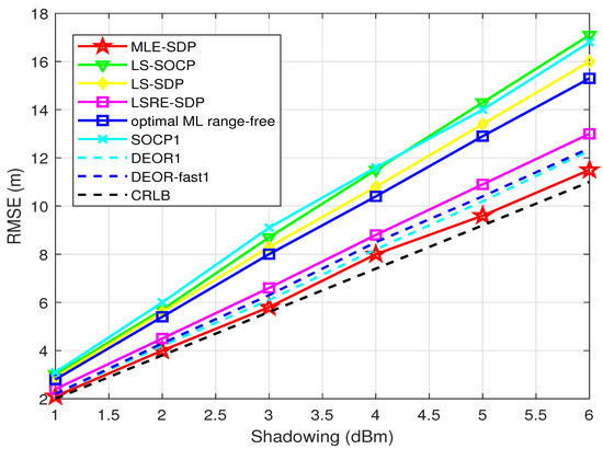
Figure 2. When $L_0$ is known, this is the relationship between RMSE and ${\sigma }_{n_i}$.

Figure 3 shows the RMSE of the estimator of the target versus the number of anchors. It is obvious that the RMSE of all algorithms reduces while the number of anchors increases. ${\sigma }_{n_i}$ is set to be 4 dBm.

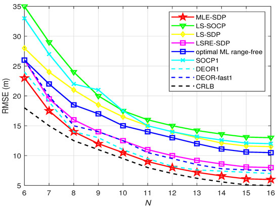
Figure 3. When $L_0$ is known, this is the relationship between RMSE and N.

As shown in Figure 3, compared with the other seven algorithms, the RMSE of the proposed algorithm is lower whether the number of anchor nodes is large or small. It is very close to the CRLB when the number of anchors is larger than 8. That means it has better performance when the number of anchor nodes is larger than 8.

Figure 4 shows the cumulative distribution function (CDF) versus the mean error (EM). The faster the CDF curve rises, the better the performance is. Nine anchors are randomly distributed, and the target is randomly generated. The standard deviation of RSS measurement noise is set as $\sigma$ = 4 dBm.

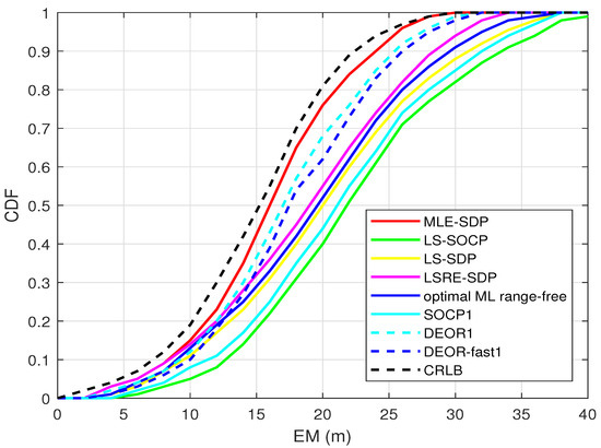
Figure 4. When $L_0$ is known, this is the CDF.

As shown in Figure 4, the CDF of the proposed algorithm is higher than the other seven algorithms. Moreover, it is the closest to the CRLB, which means it has higher accuracy.

4.2. $L_0$ Is Unknown

The average running times of the six algorithms which $L_0$ are unknown are listed in Table 5. From Table 5, we can know that the running times of the proposed algorithm “MLS-SDP2” in this paper are almost twice the running times of “MLS-SDP1”. This is due to the increase in constraints and unknown variables. The bias of the “ML-SDP2” method is 0.0768 m, according to the simulation results.

Table 5. Average running times of $L_0$ unknown situation.

Method	Describe	Running Times (s)
MLE-SDP2	The “ML-SDP2” algorithm in this paper	1.13
LS-SDP2	The “LS-SDP2” algorithm in [30]	1.65
LS-SOCP2	The “LS-SOCP2” algorithm in [31]	2.28
SOCP2	The “SOCP2” algorithm in [35]	5.43
DEOR2	The “DEOR” algorithm in [38]	0.63
DEOR-fast2	The “DEOR-fast” algorithm in [38]	0.32

First, we test the relationship between the RMSE of the estimator of the target and ${\sigma }_{n_i}$. Nine anchor nodes are randomly distributed, and the target is randomly generated. $\sigma$ change from 1 to 6.

Figure 5 shows the comparison between the proposed algorithm and other algorithms. The RMSE of all algorithms increases with the increase in the measurement noise ${\sigma }_{n_i}$, which indicates that the larger the noise, the larger the deviation of the final estimator. The proposed algorithm “MLE-SDP2” in this paper has a lower RMSE than the other five algorithms and is the closest to the CRLB. This also shows that the proposed algorithm has a significant advantage in accuracy.

Figure 5. When $L_0$ is unknown, this is the relationship between RMSE and ${\sigma }_{n_i}$.

Figure 6 shows the RMSE versus the number of anchors when $L_0$ is unknown. It is obvious that the RMSE of all algorithms reduces while the number of anchors increase. The standard deviation of RSS measurement noise is set as ${\sigma }_{n_i}$ = 4 dBm.

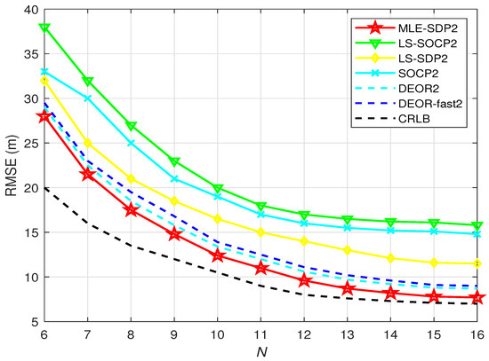
Figure 6. When $L_0$ is unknown, the relationship between RMSE versus N.

As shown in Figure 6, compared with the other five algorithms, the RMSE of the proposed algorithm is lower whether the number of anchors is large or small. It is very close to the CRLB when the number of anchor nodes is larger than 10. That means the proposed algorithm has a better performance when the anchor nodes are more than 10.

Figure 7 shows the relationship between the cumulative distribution function (CDF) and the mean error (EM). The faster the CDF curve rises, the better the performance is. Nine anchors are randomly distributed, and the target is randomly generated. The standard deviation of RSS measurement noise is set as $\sigma$ = 4 dBm.

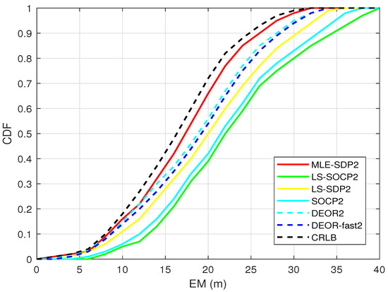
Figure 7. When $L_0$ is unknown, this is the CDF.

As shown in Figure 7, the CDF of the proposed algorithm is higher than the other two algorithms. In addition, it is the closest to the CRLB, which means it has higher accuracy.

5. Experiment

This section shows the effect of the proposed algorithm “MLE-SDP2” in the actual test. The actual test was carried out in the rectangular laboratory of 40 m long and 16 m wide. We put 8 anchor nodes and 5 target to test. The location of the anchors is fixed each time, while the location of the target is randomly placed, as shown in Figure 8. In Figure 8, the abscissa and ordinate represent the width and length of the test site, respectively. The units are both m.

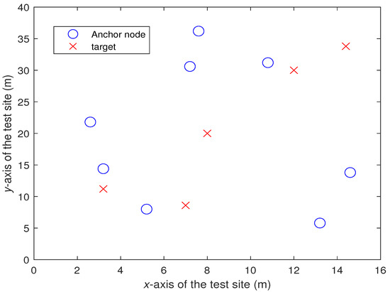
Figure 8. Distribution of the anchor nodes and the targets.

For each target, we test 100 sets of data; therefore, we collect a total of 5100 sets of data. Figure 9 shows the relationship between the cumulative distribution function (CDF) and the mean error (EM) in this experiment.

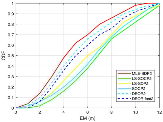
Figure 9. The CDF of the experiments.

As shown in Figure 9, the CDF of the proposed algorithm is higher than the other five algorithms. This proves the good performance of the proposed algorithm.

6. Conclusions

In this paper, a new algorithm based on maximum likelihood criterion for unknown point location using semi-definite programming estimation is studied. The estimators are proposed for the cases where $L_0$ is known and unknown. Through MATLAB simulation, the advantage of the proposed methods “MLE-SDP” and “MLE-SDP2” in calculation accuracy is confirmed. The experiments show the practicability of this algorithm. A non-line of sight (NLOS) error is the main component of measurement error. In the future work, we will model the NLOS error so that the algorithm can be better applied to practice.

References

- Shirazi, M.; Vosoughi, A. On Distributed Estimation in Hierarchical Power Constrained Wireless Sensor Networks. IEEE Trans. Signal Inf. Process. Netw. 2020, 6, 442–459. [Google Scholar] [CrossRef]
- Yin, L.; Liu, C.; Guo, S. Sparse random compressive sensing based data aggregation in wireless sensor networks. Concurr. Comp. Pract. 2020, 32, e4455. [Google Scholar] [CrossRef]
- Al-Karaki, J.; Kamal, A. Routing techniques in wireless sensor networks: A survey. IEEE Wirel. Commun. Lett. 2008, 11, 6–28. [Google Scholar] [CrossRef] [Green Version]
- Yang, T.; Niu, Y.; Yu, J. Clock Synchronization in Wireless Sensor Networks Based on Bayesian Estimation. IEEE Access 2020, 8, 69683–69694. [Google Scholar] [CrossRef]
- Pottie, G.; Kaiser, W. Wireless integrated network sensors. Commun. ACM 2000, 43, 51–58. [Google Scholar] [CrossRef]
- Anastasi, G.; Conti, M.; Di, M. Energy conservation in wireless sensor networks: A survey. AD HOC Netw. 2009, 7, 537–568. [Google Scholar] [CrossRef]
- Lu, X.; Wang, P.; Niyato, D. Wireless Networks With RF Energy Harvesting: A Contemporary Survey. IEEE Commun. Surv. Tutor. 2015, 17, 757–789. [Google Scholar] [CrossRef] [Green Version]
- Gupta, V.; De, S. Collaborative Multi-Sensing in Energy Harvesting Wireless Sensor Networks. IEEE Trans. Signal Inf. Process. Netw. 2020, 6, 426–441. [Google Scholar] [CrossRef]
- Ismail, M.; Islam, M.; Ahmad, I.; Khan, F.; Qazi, A.; Khan, Z.; Wadud, Z.; Al-Rakhami, M. Reliable Path Selection and Opportunistic Routing Protocol for Underwater Wireless Sensor Networks. IEEE Access 2020, 8, 100346–100364. [Google Scholar] [CrossRef]
- Younis, M.; Akkaya, K. Strategies and techniques for node placement in wireless sensor networks: A survey. AD HOC Netw. 2008, 6, 621–655. [Google Scholar] [CrossRef]
- Khan, A.N.; Tariq, M.A.; Asim, M.; Maamar, Z.; Baker, T. Congestion avoidance in wireless sensor network using software defined network. Computing 2021, 103, 2573–2596. [Google Scholar] [CrossRef]
- Alanezi, M.A.; Bouchekara, H.R.E.H.; Javaid, M.S.; Maamar, Z. Range-Based Localization of a Wireless Sensor Network for Internet of Things Using Received Signal Strength Indicator and the Most Valuable Player Algorithm. Sensors 2021, 9, 42. [Google Scholar] [CrossRef]
- Wang, W.; Liu, X.; Li, M.; Wang, Z.; Wang, C. Optimizing Node Localization in Wireless Sensor Networks Based on Received Signal Strength Indicator. IEEE Access 2019, 7, 73880–73889. [Google Scholar] [CrossRef]
- Dogancay, K.; Hmam, H. Optimal angular sensor separation for AOA localization. Signal Process. 2008, 88, 1248–1260. [Google Scholar] [CrossRef]
- Chuang, S.; Wu, W.; Liu, Y. High-Resolution AoA Estimation for Hybrid Antenna Arrays. IEEE Trans. Antennas Propag. 2015, 63, 2955–2968. [Google Scholar] [CrossRef]
- Sheng, H.; Wu, W. AoA Estimation With Hybrid Antenna Arrays. IEEE Trans. Wirel. Commun. 2021, 20, 5058–5070. [Google Scholar] [CrossRef]
- Monfared, S.; Copa, E.; De, D.; Horlin, F. AoA-Based Iterative Positioning of IoT Sensors With Anchor Selection in NLOS Environments. IEEE Trans. Veh. Technol. 2021, 70, 6211–6216. [Google Scholar]
- Chen, H.; Wang, G.; Wu, X. Cooperative Multiple Target Nodes Localization Using TOA in Mixed LOS/NLOS Environments. IEEE Sens. J. 2020, 20, 1473–1484. [Google Scholar] [CrossRef]
- Shi, J.; Wang, G.; Jin, L. Moving source localization using TOA and FOA measurements with imperfect synchronization. Signal Proces. 2021, 186, 108113. [Google Scholar] [CrossRef]
- Wu, S.; Zhang, S.; Huang, D. A TOA-Based Localization Algorithm With Simultaneous NLOS Mitigation and Synchronization Error Elimination. IEEE Sens. Lett. 2019, 3, 18509046. [Google Scholar] [CrossRef]
- Wang, G.; Chen, H.; Zhu, W.; Ansari, N. Robust TDOA-Based Localization for IoT via Joint Source Position and NLOS Error Estimation. IEEE Internet Things J. 2019, 6, 8529–8541. [Google Scholar] [CrossRef]
- Zhou, Z.; Rui, Y.; Cai, X. Constrained total least squares method using TDOA measurements for jointly estimating acoustic emission source and wave velocity. Measurement 2021, 182, 109758. [Google Scholar] [CrossRef]
- Kumar, S. Performance Analysis of RSS-Based Localization in Wireless Sensor Networks. Wirel. Pers. Commun. 2019, 108, 769–783. [Google Scholar] [CrossRef]
- Ababneh, A. Low-Complexity Bit Allocation for RSS Target Localization. IEEE Sens. J. 2019, 19, 7733–7743. [Google Scholar] [CrossRef]
- He, Z.; Li, Y.; Pei, L.; Chen, R.; El-Sheimy, N. Calibrating Multi-Channel RSS Observations for Localization Using Gaussian Process. IEEE Wirel. Commun. Lett. 2019, 8, 1116–1119. [Google Scholar] [CrossRef]
- Abed, A.; Abdel, I. RSS-Fingerprint Dimensionality Reduction for Multiple Service Set Identifier-Based Indoor Positioning Systems. Appl. Sci. 2019, 9, 3137. [Google Scholar] [CrossRef] [Green Version]
- Nguyen, T.; Shin, Y. An Efficient RSS Localization for Underwater Wireless Sensor Networks. Sensors 2019, 19, 3105. [Google Scholar] [CrossRef] [Green Version]
- Wielandner, L.; Leitinger, E.; Witrisal, K. RSS-Based Cooperative Localization and Orientation Estimation Exploiting Antenna Directivity. IEEE Access 2021, 9, 53046–53060. [Google Scholar] [CrossRef]
- Janssen, T.; Berkvens, R.; Weyn, M. RSS-Based Localization and Mobility Evaluation Using a Single NB-IoT Cell dagger. Sensors 2020, 20, 6172. [Google Scholar] [CrossRef]
- Robin, W.; Albert, K.; Chin-Tau, L. Received Signal Strength-Based Wireless Localization via Semidefinite Programming: Noncooperative and Cooperative Schemes. IEEE Trans. Veh. Technol. 2010, 59, 1307–1318. [Google Scholar]
- Tomic, S.; Marko, B.; Rui, D.; Vlatko, L. RSS-based Localization in Wireless Sensor Networks using SOCP Relaxation. In Proceedings of the IEEE 14th Workshop on Signal Processing Advances in Wireless Communications, Darmstadt, Germany, 16–19 June 2013. [Google Scholar]
- Wang, Z.; Zhang, H.; Lu, T.; Aaron, T. Cooperative RSS-Based Localization in Wireless Sensor Networks Using Relative Error Estimation and Semidefinite Programming. IEEE Trans. Veh. Technol. 2018, 68, 483–497. [Google Scholar] [CrossRef]
- Prasad, K.; Bhargava, V. RSS Localization Under Gaussian Distributed Path Loss Exponent Model. IEEE Wirel. Commun. Lett. 2021, 10, 111–115. [Google Scholar] [CrossRef]
- Mei, X.; Wu, H.; Xian, J.; Chen, B. RSS-based Byzantine Fault-tolerant Localization Algorithm under NLOS Environment. IEEE Wirel. Commun. Lett. 2021, 25, 474–478. [Google Scholar] [CrossRef]
- Tomic, S.; Beko, M.; Dinis, R. RSS-Based Localization in Wireless Sensor Networks Using Convex Relaxation: Noncooperative and Cooperative Schemes. IEEE Trans. Veh. Technol. 2015, 64, 2037–2050. [Google Scholar] [CrossRef] [Green Version]
- Chang, S.; Li, Y.; Wang, H.; Hu, W.; Wu, Y. RSS-Based Cooperative Localization in Wireless Sensor Networks via Second-Order Cone Relaxation. IEEE Access 2018, 6, 54097–54105. [Google Scholar] [CrossRef]
- Coluccia, A.; Ricciato, F. RSS-based Localization via Bayesian Ranging and Iterative Least Squares Positioning. IEEE Wirel. Commun. Lett. 2014, 18, 873–876. [Google Scholar] [CrossRef]
- Najarro, L.A.C.; Song, L.; Kim, K. Differential Evolution With Opposition and Redirection for Source Localization Using RSS Measurements in Wireless Sensor Networks. IEEE Trans. Autom. Sci. Eng. 2020, 17, 1736–1747. [Google Scholar] [CrossRef]
- Najarro, L.A.C.; Song, L.; Tomic, S.; Kim, K. Fast Localization With Unknown Transmit Power and Path-Loss Exponent in WSNs Based on RSS Measurements. IEEE Wirel. Commun. Lett. 2020, 24, 2756–2760. [Google Scholar] [CrossRef]
- Boyd, S.; Vandenberghe, L. Convex Optimization; Cambridge University Press: Cambridge, MA, USA, 2004. [Google Scholar]
Publisher’s Note: MDPI stays neutral with regard to jurisdictional claims in published maps and institutional affiliations. |
© 2022 by the authors. Licensee MDPI, Basel, Switzerland. This article is an open access article distributed under the terms and conditions of the Creative Commons Attribution (CC BY) license (https://creativecommons.org/licenses/by/4.0/).