
LidSonic V2.0: A LiDAR and Deep-Learning-Based Green Assistive Edge Device to Enhance Mobility for the Visually Impaired

 ,
,  ,
,  ,
,  and
and 
Abstract
1. Introduction
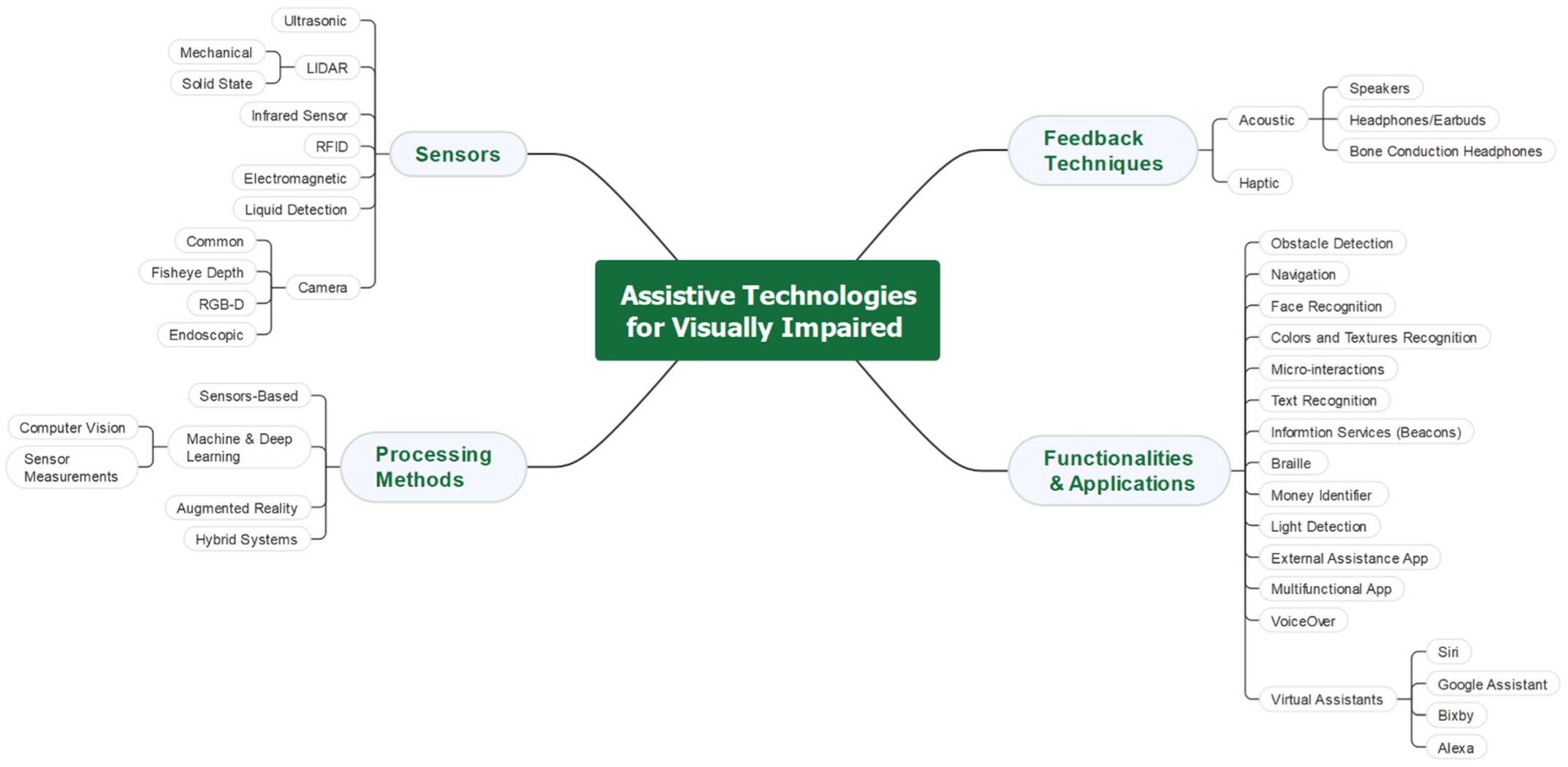
2. Related Work
2.1. Sensor Technologies and Types Used in Assistive Tools
2.1.1. Ultrasonic Sensors
2.1.2. LiDAR Sensors
2.1.3. Infrared (IR) Sensors
2.1.4. RFID Sensors
2.1.5. Electromagnetic Sensors (Microwave Radar)
2.1.6. Liquid Detection Sensors
2.1.7. Cameras

| Sensor Name | Works | Purpose of Sensor | No. of Sensors | Weight | Wearable/Assistive | Feedback Method |
|---|---|---|---|---|---|---|
| IR Sensors | [58] | Touch down, touch up sensor | 2 | Light | Mounted on top of a finger | Acoustic |
| [49] | Detect obstacles, stairs | 2 | Light | Cane | Acoustic | |
| IMU | [58] | Recognize gestures and sense movements | 1 | Light | Mounted on top of a finger | Acoustic |
| Ultrasonic Sensors | [23] | Detect obstacles up to the chest level | 5 | Light | Cane | Acoustic, vibration |
| [59] | Detect obstacles | 2 | High | Guide dog robot and portable robot | Acoustic | |
| [45] | Detect obstacles | 5 | Fair | Mounted on the head, legs, and arms | Buzzer, vibration | |
| [44] | Detect obstacles | 2 | Fair | Belt | Vibration | |
| ToF Distance Sensors | [12] | Detect obstacles | 7 | High | Belt | Vibration belt |
| Microwave Radar | [37] | Detect obstacles | 1 | Light | Mounted on a cane | Acoustic, vibration |
| Wet Floor Detection Sensors | [53] | Detect wet floors | 1 | Light | Cane | Buzzer |
| Bluetooth | [60] | Informing about indoor environments | 3 | Light | Beacon transmitter, smartphone | Acoustic |
| Laser Pointer | [61] | Detect obstacles | 1 | Light | Belt | Vibration belt |
| Cameras | [58] | Localize the hand touch | 1 | Light | Mounted on top of a finger | Acoustic |
| [62] | Emotion recognition | 1 | Light | Clipped on to spectacles | Vibration belt | |
| [59] | Obstacle recognition (traffic light, cones, bus, etc.) | 2 | High | Guide dog robot and portable robot | Acoustic | |
| [63] | Localization system | 1 | Low | Head level (helmet), chest level (hanged) | Location in a Map | |
| RGB-D Cameras | [61] | Detect obstacles | 1 | Light | Smartphone simulating a cane | Vibratory belt |
| [64] | Avoid obstacles, localization system for indoor navigation | 1 | Light | Glass, tactile vest, smartphone | Haptic vest (4 vibration motors) | |
| Endoscopic Cameras | [65] | Identify clothing colors, visual texture recognition | 1 | Light | Mounted on top of a finger | Acoustic |
| Compass | [66] | Indoor navigation | 1 | Light | Optical head-mounted (Glass) | Acoustic |
2.2. Processing Methods
2.3. Feedback Techniques
2.3.1. Haptics
2.3.2. Acoustic
2.4. Functions and Applications
2.4.1. Obstacle Detection
2.4.2. Navigation
2.4.3. Facial and Emotion Recognition
2.4.4. Color and Texture Recognition
2.4.5. Micro-Interactions
2.4.6. Text Recognition
2.4.7. Information Services
2.4.8. Braille Display and Printer
2.4.9. Money Identifier App
2.4.10. Light Detection
2.4.11. External Assistance App
2.4.12. Multifunctional App
2.4.13. VoiceOver
2.4.14. Virtual Assistant Apps (Voice Commands)
Siri
Google Assistant
Bixby
Alexa
2.5. Research Gap
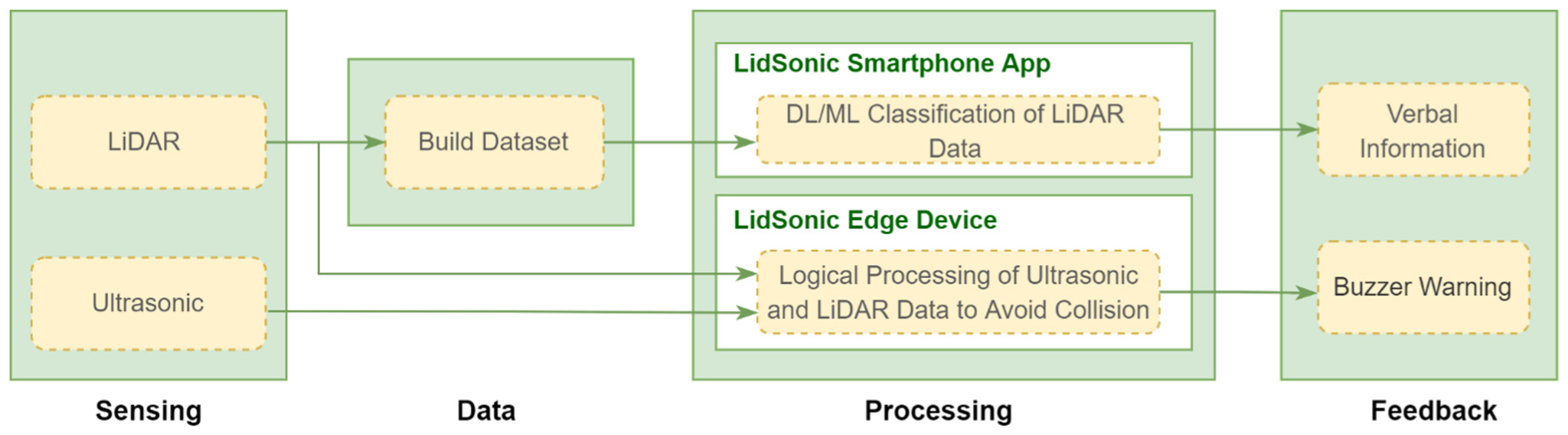
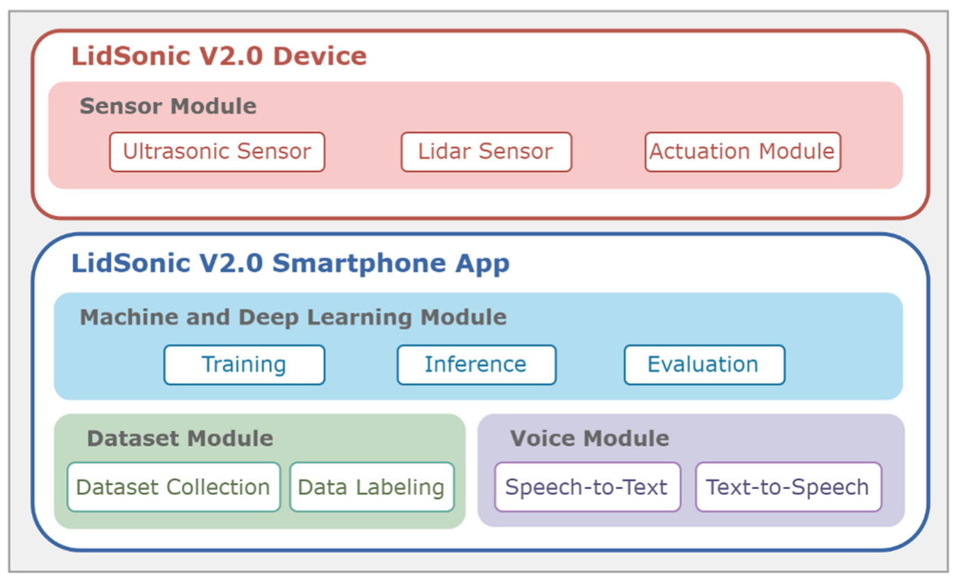
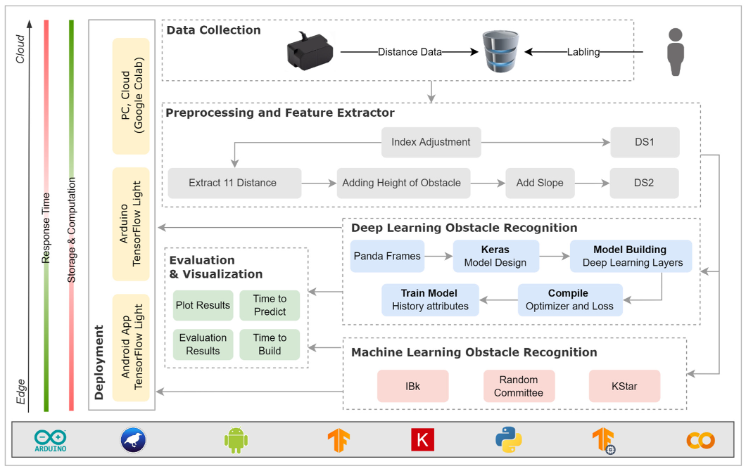
3. A High-Level View
3.1. User View
3.2. Developer View
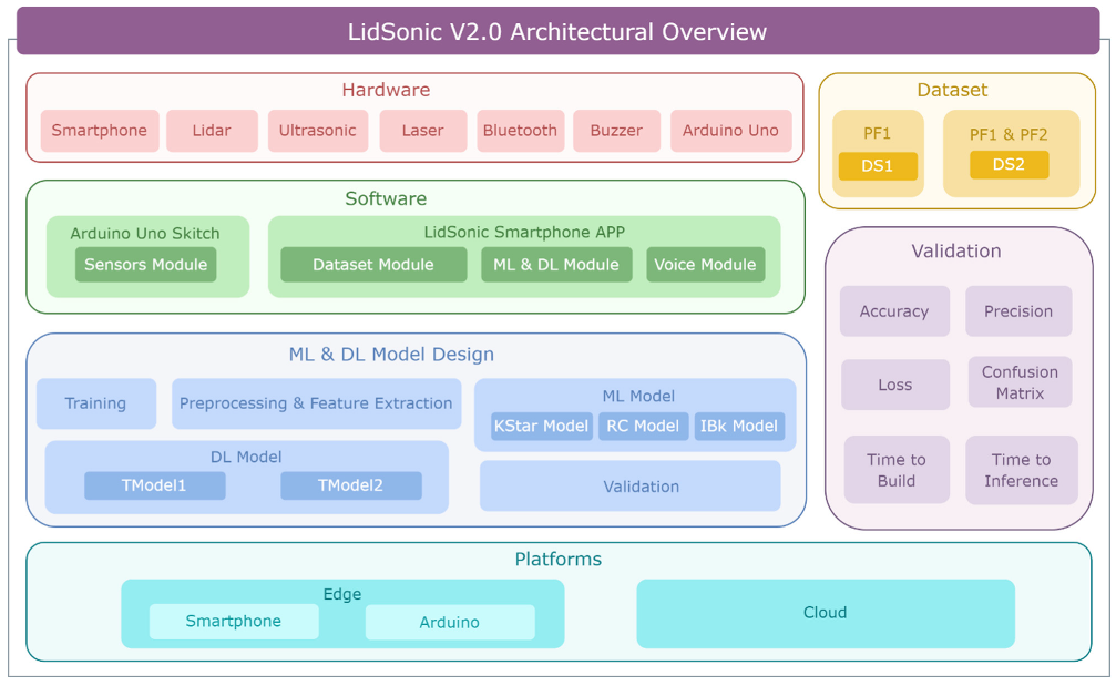
3.3. System View
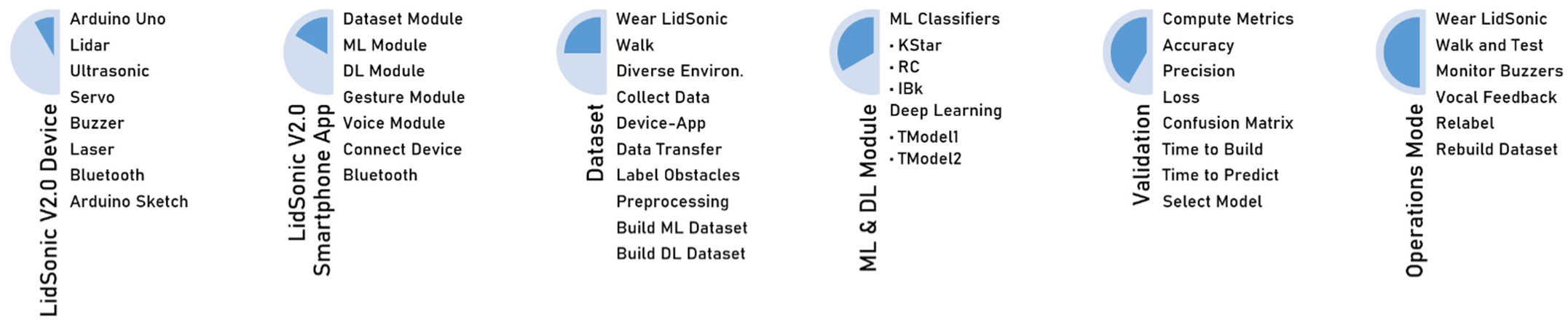
4. Design and Implementation
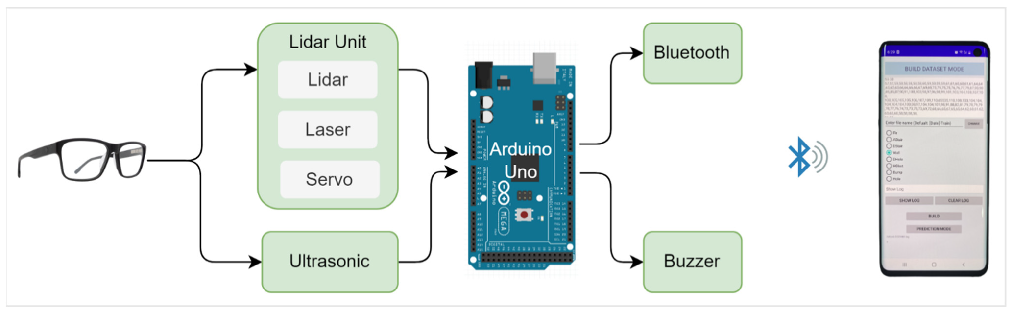
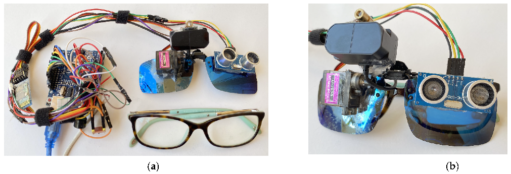
4.1. System Hardware
4.1.1. TFmini-S LiDAR
4.1.2. Ultrasonic Sensor
4.2. System Software
| Algorithm1: The Master algorithm: LidSonic V2.0 |
| Input: VoiceCommands (Label, Relabel, VoiceOff, VoiceOn, Classify), AIType (ML, DL) Output: LFalert, HFalert, VoiceFeedback
|
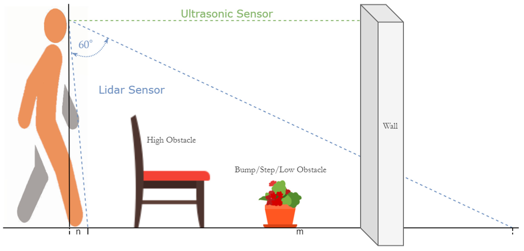
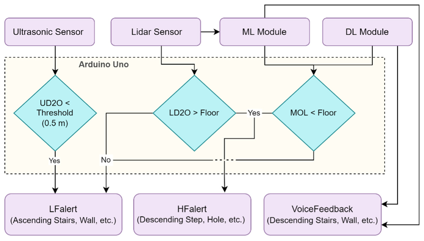
4.3. Sensor Module
| Algorithm2: Obstacle Detection, Warning, and Feedback |
| Input: UD2O, LD2O, MOL, DOL Output: FeedbackType (HFalert, LFalert, VoiceFeedback)
|
4.4. Dataset Module

| Algorithm3: DatasetModule: Building Dataset Algorithm |
| Input: Header, LDO Output: Dataset
|
4.5. Machine and Deep Learning Module
| Algorithm4: PreProFXModuleDL: Preprocessing and Feature Extraction |
| Input: Dataset, LIndex1, LIndex2 Output: Dataset
|
| Algorithm 5: Machine learning Module |
| Input: Dataset, PrFx Output: MOL, VoiceCommands
|
| Algorithm 6: Deep Learning Module |
| Input: Dataset, PrFx Output: DOL, VoiceCommands
|
4.5.1. Machine Learning Models (WEKA)
KStar Algorithm
Instance-Based Learner (IBk) Algorithm
Random Committee Algorithm
4.5.2. Deep Learning Models: TensorFlow
ReLU
Softmax Regression
Cost Function
Adam Optimizer
4.6. Voice Module
5. Performance Evaluation
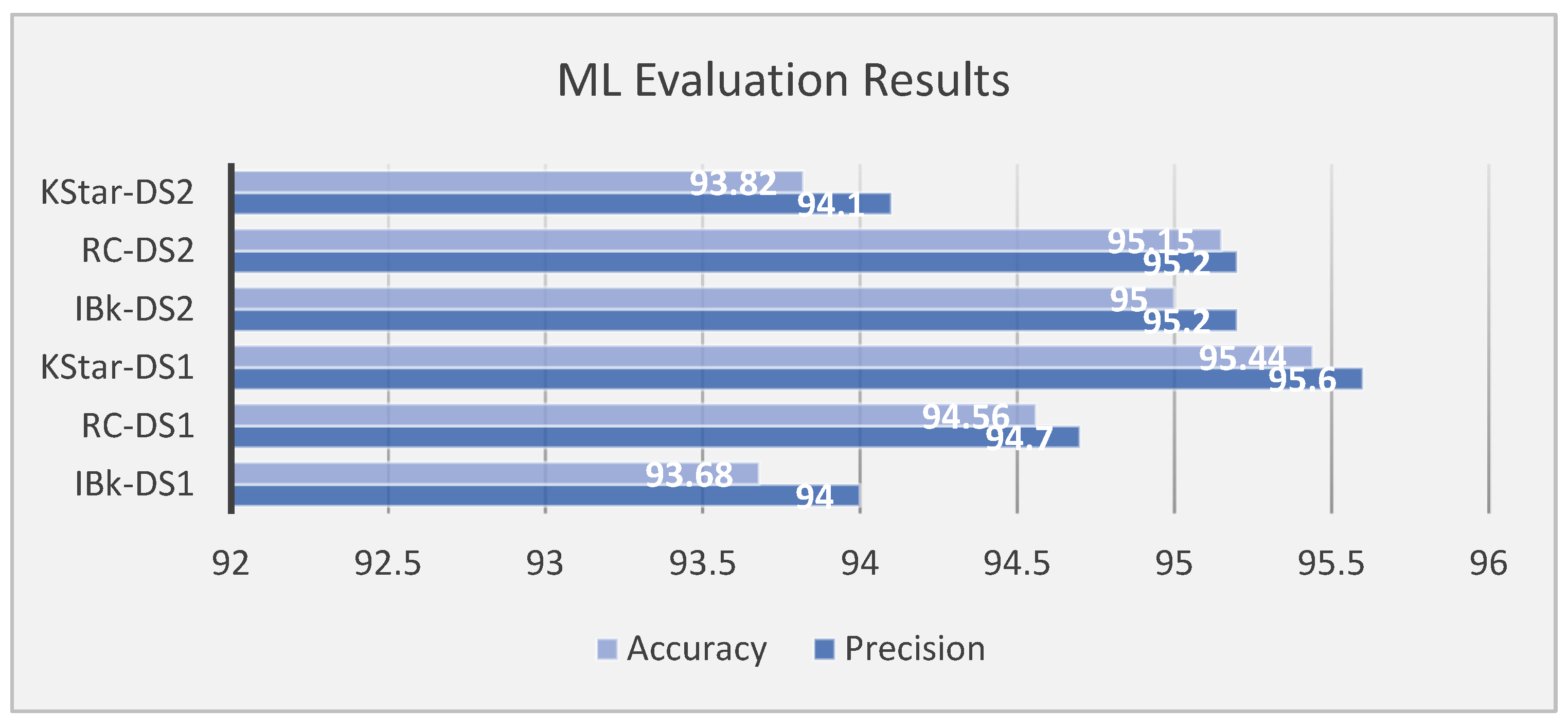
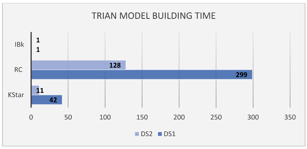
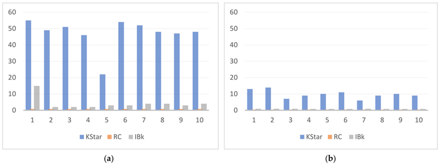
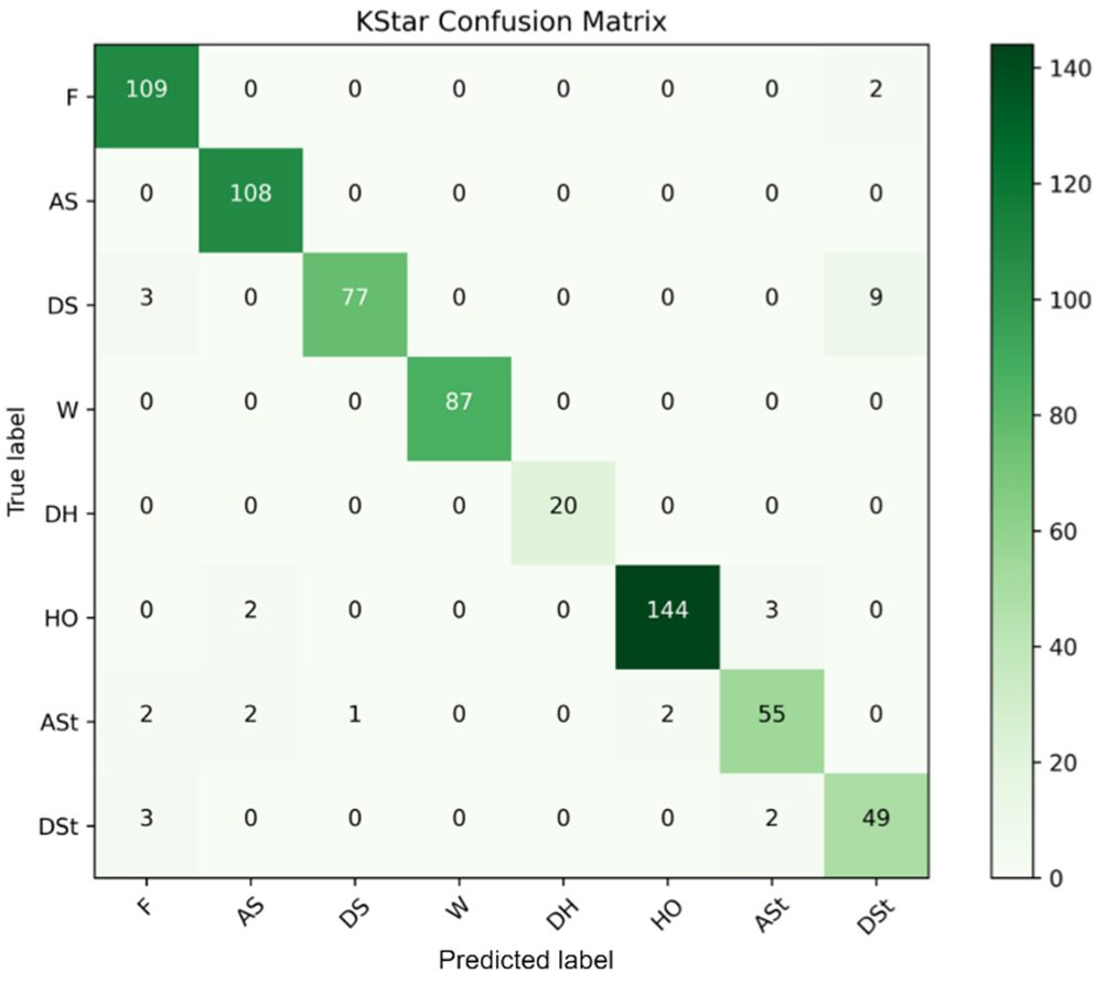
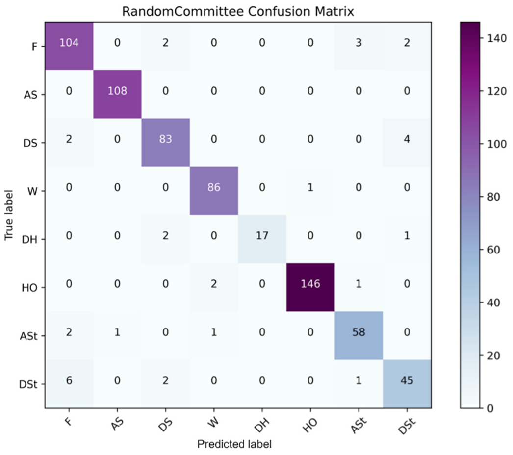
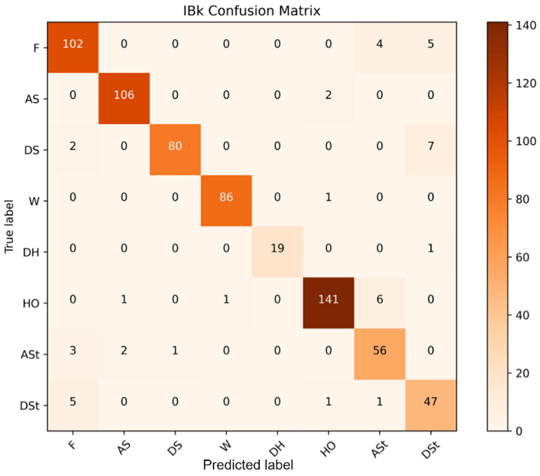
5.1. Machine-Learning-Based Performance
5.2. Deep-Learning-Based Performance
6. Conclusions
Author Contributions
Funding
Institutional Review Board Statement
Informed Consent Statement
Data Availability Statement
Acknowledgments
Conflicts of Interest
Abbreviations
| ETA | Electronic Travel Aids |
| ToF | Time-of-flight |
| RNA | Robotic Navigation Aid |
| ALVU | Array of LiDARs and Vibrotactile Units |
| BLE | Bluetooth Low Energy |
| SDK | Software Development Kit |
| RGB-D | RGB-Depth |
| CNN | Convolutional Neural Networks |
| RFID | Radio Frequency Identification Reader |
| HRTFs | Head-Related Transfer Functions |
| GPS | Global Positioning System |
| MSER | Maximally Stable External Region |
| SWT | Stroke Width Transform |
References
- World Health Organisation (WHO). Disability and Health (24 November 2021). Available online: https://www.who.int/news-room/fact-sheets/detail/disability-and-health (accessed on 19 July 2022).
- World Health Organisation (WHO). Disability. Available online: https://www.who.int/health-topics/disability#tab=tab_1 (accessed on 19 July 2022).
- DISABLED | Meaning in the Cambridge English Dictionary. Available online: https://dictionary.cambridge.org/dictionary/english/disabled (accessed on 7 February 2020).
- Physical Disability—Wikipedia. Available online: https://en.wikipedia.org/wiki/Physical_disability (accessed on 30 July 2022).
- Disability and Health Overview|CDC. Available online: https://www.cdc.gov/ncbddd/disabilityandhealth/disability.html (accessed on 30 July 2022).
- Disability Facts and Figures|Disability Charity Scope UK. Available online: https://www.scope.org.uk/media/disability-facts-figures/ (accessed on 30 July 2022).
- Disability among People in the U.S. 2008–2019|Statista. Available online: https://www.statista.com/statistics/792697/disability-in-the-us-population-share/ (accessed on 30 July 2022).
- Disabled People in the World: Facts and Figures. Available online: https://www.inclusivecitymaker.com/disabled-people-in-the-world-in-2021-facts-and-figures/ (accessed on 30 July 2022).
- Questions and Answers about Blindness and Vision Impairments in the Workplace and the Americans with Disabilities Act|U.S. Equal Employment Opportunity Commission. Available online: https://www.eeoc.gov/fact-sheet/questions-and-answers-about-blindness-and-vision-impairments-workplace-and-americans (accessed on 8 June 2020).
- Blind vs. Visually Impaired: What’s the Difference?|IBVI|Blog. Available online: https://ibvi.org/blog/blind-vs-visually-impaired-whats-the-difference/ (accessed on 8 June 2020).
- What Is Visual Impairment? Available online: https://www.news-medical.net/health/What-is-visual-impairment.aspx (accessed on 8 June 2020).
- Katzschmann, R.K.; Araki, B.; Rus, D. Safe local navigation for visually impaired users with a time-of-flight and haptic feedback device. IEEE Trans. Neural Syst. Rehabil. Eng. 2018, 26, 583–593. [Google Scholar] [CrossRef] [PubMed]
- Alotaibi, S.; Mehmood, R.; Katib, I.; Rana, O.; Albeshri, A. Sehaa: A Big Data Analytics Tool for Healthcare Symptoms and Diseases Detection Using Twitter, Apache Spark, and Machine Learning. Appl. Sci. 2020, 10, 1398. [Google Scholar] [CrossRef]
- Praveen Kumar, M.; Poornima; Mamidala, E.; Al-Ghanim, K.; Al-Misned, F.; Ahmed, Z.; Mahboob, S. Effects of D-Limonene on aldose reductase and protein glycation in diabetic rats. J. King Saud Univ.—Sci. 2020, 32, 1953–1958. [Google Scholar] [CrossRef]
- Ekstrom, A.D. Why vision is important to how we navigate. Hippocampus 2015, 25, 731–735. [Google Scholar] [CrossRef]
- Deverell, L.; Bentley, S.A.; Ayton, L.N.; Delany, C.; Keeffe, J.E. Effective mobility framework: A tool for designing comprehensive O&M outcomes research. IJOM 2015, 7, 74–86. [Google Scholar]
- Andò, B. Electronic sensory systems for the visually impaired. IEEE Instrum. Meas. Mag. 2003, 6, 62–67. [Google Scholar] [CrossRef]
- Ranaweera, P.S.; Madhuranga, S.H.R.; Fonseka, H.F.A.S.; Karunathilaka, D.M.L.D. Electronic travel aid system for visually impaired people. In Proceedings of the 2017 5th International Conference on Information and Communication Technology (ICoIC7), Melaka, Malaysia, 17–19 May 2017; IEEE: Piscataway, NJ, USA, 2017. [Google Scholar] [CrossRef]
- Bindawas, S.M.; Vennu, V. The National and Regional Prevalence Rates of Disability, Type, of Disability and Severity in Saudi Arabia-Analysis of 2016 Demographic Survey Data. Int. J. Environ. Res. Public Health 2018, 15, 419. [Google Scholar] [CrossRef]
- General Authority for Statistics. GaStat: (2.9%) of Saudi Population Have Disability with (Extreme) Difficulty. Available online: https://www.stats.gov.sa/en/news/230 (accessed on 30 July 2022).
- Patel, S.; Kumar, A.; Yadav, P.; Desai, J.; Patil, D. Smartphone-based obstacle detection for visually impaired people. In Proceedings of the 2017 International Conference on Innovations in Information, Embedded and Communication Systems (ICIIECS), Coimbatore, India, 17–18 March 2017; IEEE: Piscataway, NJ, USA, 2018. [Google Scholar] [CrossRef]
- Rizzo, J.R.; Pan, Y.; Hudson, T.; Wong, E.K.; Fang, Y. Sensor fusion for ecologically valid obstacle identification: Building a comprehensive assistive technology platform for the visually impaired. In Proceedings of the 2017 7th International Conference on Modeling, Simulation, and Applied Optimization (ICMSAO), Sharjah, United Arab Emirates, 4–6 April 2017; Institute of Electrical and Electronics Engineers Inc.: Piscataway, NJ, USA, 2017. [Google Scholar]
- Meshram, V.V.; Patil, K.; Meshram, V.A.; Shu, F.C. An Astute Assistive Device for Mobility and Object Recognition for Visually Impaired People. IEEE Trans. Hum.-Mach. Syst. 2019, 49, 449–460. [Google Scholar] [CrossRef]
- Omoregbee, H.O.; Olanipekun, M.U.; Kalesanwo, A.; Muraina, O.A. Design and Construction of A Smart Ultrasonic Walking Stick for the Visually Impaired. In Proceedings of the 2021 Southern African Universities Power Engineering Conference/Robotics and Mechatronics/Pattern Recognition Association of South Africa (SAUPEC/RobMech/PRASA), Potchefstroom, South Africa, 27–29 January 2021. [Google Scholar] [CrossRef]
- Mehmood, R.; See, S.; Katib, I.; Chlamtac, I. Smart Infrastructure and Applications: Foundations for Smarter Cities and Societies; Springer International Publishing, Springer Nature: Cham, Switzerland, 2020; ISBN 9783030137045. [Google Scholar]
- Yigitcanlar, T.; Butler, L.; Windle, E.; Desouza, K.C.; Mehmood, R.; Corchado, J.M. Can Building “Artificially Intelligent Cities” Safeguard Humanity from Natural Disasters, Pandemics, and Other Catastrophes? An Urban Scholar’s Perspective. Sensors 2020, 20, 2988. [Google Scholar] [CrossRef]
- Mehmood, R.; Bhaduri, B.; Katib, I.; Chlamtac, I. Smart Societies, Infrastructure, Technologies and Applications. In Proceedings of the Smart Societies, Infrastructure, Technologies and Applications, Lecture Notes of the Institute for Computer Sciences, Social Informatics and Telecommunications Engineering (LNICST), Jeddah, Saudi Arabia, 27–29 November 2017; Springer International Publishing: Cham, Switzerland, 2018; Volume 224. [Google Scholar]
- Mehmood, R.; Sheikh, A.; Catlett, C.; Chlamtac, I. Editorial: Smart Societies, Infrastructure, Systems, Technologies, and Applications. Mob. Netw. Appl. 2022, 1, 1–5. [Google Scholar] [CrossRef]
- Electronic Travel Aids for the Blind. Available online: https://www.tsbvi.edu/orientation-and-mobility-items/1974-electronic-travel-aids-for-the-blind (accessed on 5 February 2020).
- INTRODUCTION—Electronic Travel AIDS: New Directions for Research—NCBI Bookshelf. Available online: https://www.ncbi.nlm.nih.gov/books/NBK218018/ (accessed on 5 February 2020).
- Bai, J.; Lian, S.; Liu, Z.; Wang, K.; Liu, D. Smart guiding glasses for visually impaired people in indoor environment. IEEE Trans. Consum. Electron. 2017, 63, 258–266. [Google Scholar] [CrossRef]
- Islam, M.M.; Sadi, M.S.; Zamli, K.Z.; Ahmed, M.M. Developing Walking Assistants for Visually Impaired People: A Review. IEEE Sens. J. 2019, 19, 2814–2828. [Google Scholar] [CrossRef]
- Siddesh, G.M.; Srinivasa, K.G. IoT Solution for Enhancing the Quality of Life of Visually Impaired People. Int. J. Grid High Perform. Comput. 2021, 13, 1–23. [Google Scholar] [CrossRef]
- Mallikarjuna, G.C.P.; Hajare, R.; Pavan, P.S.S. Cognitive IoT System for visually impaired: Machine Learning Approach. Mater. Today Proc. 2021, 49, 529–535. [Google Scholar] [CrossRef]
- Stearns, L.; DeSouza, V.; Yin, J.; Findlater, L.; Froehlich, J.E. Augmented reality magnification for low vision users with the microsoft hololens and a finger-worn camera. In Proceedings of the 19th International ACM SIGACCESS Conference on Computers and Accessibility, Baltimore, MD, USA, 29 October–1 November 2017; pp. 361–362. [Google Scholar] [CrossRef]
- Busaeed, S.; Mehmood, R.; Katib, I. Requirements, Challenges, and Use of Digital Devices and Apps for Blind and Visually Impaired. Preprints 2022, 2022070068. [Google Scholar] [CrossRef]
- Cardillo, E.; Di Mattia, V.; Manfredi, G.; Russo, P.; De Leo, A.; Caddemi, A.; Cerri, G. An Electromagnetic Sensor Prototype to Assist Visually Impaired and Blind People in Autonomous Walking. IEEE Sens. J. 2018, 18, 2568–2576. [Google Scholar] [CrossRef]
- O’Keeffe, R.; Gnecchi, S.; Buckley, S.; O’Murchu, C.; Mathewson, A.; Lesecq, S.; Foucault, J. Long Range LiDAR Characterisation for Obstacle Detection for use by the Visually Impaired and Blind. In Proceedings of the 2018 IEEE 68th Electronic Components and Technology Conference (ECTC), San Diego, CA, USA, 29 May–1 June 2018; Institute of Electrical and Electronics Engineers Inc.: Piscataway, NJ, USA, 2018; pp. 533–538. [Google Scholar]
- Busaeed, S.; Mehmood, R.; Katib, I.; Corchado, J.M. LidSonic for Visually Impaired: Green Machine Learning-Based Assistive Smart Glasses with Smart App and Arduino. Electronics 2022, 11, 1076. [Google Scholar] [CrossRef]
- Magori, V. Ultrasonic sensors in air. In Proceedings of the IEEE Ultrasonics Symposium, Cannes, France, 31 October–3 November 1994; IEEE: Piscataway, NJ, USA, 1994; Volume 1, pp. 471–481. [Google Scholar]
- Different Types of Sensors, Applications. Available online: https://www.electronicshub.org/different-types-sensors/ (accessed on 8 March 2020).
- Fauzul, M.A.H.; Salleh, N.D.H.M. Navigation for the Vision Impaired with Spatial Audio and Ultrasonic Obstacle Sensors. In Proceedings of the International Conference on Computational Intelligence in Information System, Bandar Seri Begawan, Brunei Darussalam, 25–27 January 2021; Springer: Cham, Switzerland, 2021; pp. 43–53. [Google Scholar] [CrossRef]
- Gearhart, C.; Herold, A.; Self, B.; Birdsong, C.; Slivovsky, L. Use of Ultrasonic sensors in the development of an Electronic Travel Aid. In Proceedings of the SAS 2009—IEEE Sensors Applications Symposium Proceedings, New Orleans, LA, USA, 17–19 February 2009; pp. 275–280. [Google Scholar]
- Tudor, D.; Dobrescu, L.; Dobrescu, D. Ultrasonic electronic system for blind people navigation. In Proceedings of the 2015 E-Health and Bioengineering Conference, EHB, Lasi, Romania, 19–21 November 2015; Institute of Electrical and Electronics Engineers Inc.: Piscataway, NJ, USA, 2016. [Google Scholar]
- Khan, A.A.; Khan, A.A.; Waleed, M. Wearable navigation assistance system for the blind and visually impaired. In Proceedings of the 2018 International Conference on Innovation and Intelligence for Informatics, Computing, and Technologies, 3ICT, Sakhier, Bahrain, 18–20 November 2018; Institute of Electrical and Electronics Engineers Inc.: Piscataway, NJ, USA, 2018. [Google Scholar]
- Noman, A.T.; Chowdhury, M.A.M.; Rashid, H.; Faisal, S.M.S.R.; Ahmed, I.U.; Reza, S.M.T. Design and implementation of microcontroller based assistive robot for person with blind autism and visual impairment. In Proceedings of the 20th International Conference of Computer and Information Technology, ICCIT, Dhaka, Bangladesh, 22–24 December 2017; Institute of Electrical and Electronics Engineers Inc.: Piscataway, NJ, USA, 2018; pp. 1–5. [Google Scholar]
- Chitra, P.; Balamurugan, V.; Sumathi, M.; Mathan, N.; Srilatha, K.; Narmadha, R. Voice Navigation Based Guiding Device for Visually Impaired People. In Proceedings of the 2021 International Conference on Artificial Intelligence and Smart Systems (ICAIS), Coimbatore, India, 25–27 March 2021; pp. 911–915. [Google Scholar] [CrossRef]
- What Is an IR Sensor?|FierceElectronics. Available online: https://www.fierceelectronics.com/sensors/what-ir-sensor (accessed on 16 March 2020).
- Nada, A.A.; Fakhr, M.A.; Seddik, A.F. Assistive infrared sensor based smart stick for blind people. In Proceedings of the Proceedings of the 2015 Science and Information Conference, SAI, London, UK, 28–30 July 2015; Institute of Electrical and Electronics Engineers Inc.: Piscataway, NJ, USA, 2015; pp. 1149–1154. [Google Scholar]
- Elmannai, W.; Elleithy, K. Sensor-Based Assistive Devices for Visually-Impaired People: Current Status, Challenges, and Future Directions. Sensors 2017, 17, 565. [Google Scholar] [CrossRef]
- Chaitrali, K.S.; Yogita, D.A.; Snehal, K.K.; Swati, D.D.; Aarti, D.V. An Intelligent Walking Stick for the Blind. Int. J. Eng. Res. Gen. Sci. 2015, 3, 1057–1062. [Google Scholar]
- Cardillo, E.; Li, C.; Caddemi, A. Millimeter-Wave Radar Cane: A Blind People Aid with Moving Human Recognition Capabilities. IEEE J. Electromagn. RF Microw. Med. Biol. 2021, 6, 204–211. [Google Scholar] [CrossRef]
- Ikbal, M.A.; Rahman, F.; Hasnat Kabir, M. Microcontroller based smart walking stick for visually impaired people. In Proceedings of the 4th International Conference on Electrical Engineering and Information and Communication Technology, iCEEiCT, Dhaka, Bangladesh, 13–15 September 2018; Institute of Electrical and Electronics Engineers Inc.: Piscataway, NJ, USA, 2019; pp. 255–259. [Google Scholar]
- Gbenga, D.E.; Shani, A.I.; Adekunle, A.L. Smart Walking Stick for Visually Impaired People Using Ultrasonic Sensors and Arduino. Int. J. Eng. Technol. 2017, 9, 3435–3447. [Google Scholar] [CrossRef]
- Yang, K.; Wang, K.; Cheng, R.; Hu, W.; Huang, X.; Bai, J. Detecting Traversable Area and Water Hazards for the Visually Impaired with a pRGB-D Sensor. Sensors 2017, 17, 1890. [Google Scholar] [CrossRef]
- Ye, C.; Qian, X. 3-D Object Recognition of a Robotic Navigation Aid for the Visually Impaired. IEEE Trans. Neural Syst. Rehabil. Eng. 2018, 26, 441–450. [Google Scholar] [CrossRef]
- Cornacchia, M.; Kakillioglu, B.; Zheng, Y.; Velipasalar, S. Deep Learning-Based Obstacle Detection and Classification with Portable Uncalibrated Patterned Light. IEEE Sens. J. 2018, 18, 8416–8425. [Google Scholar] [CrossRef]
- Oh, U.; Stearns, L.; Pradhan, A.; Froehlich, J.E.; Indlater, L.F. Investigating microinteractions for people with visual impairments and the potential role of on-body interaction. In Proceedings of the 19th International ACM SIGACCESS Conference on Computers and Accessibility, Baltimore, MD, USA, 29 October–1 November 2017; pp. 22–31. [Google Scholar] [CrossRef]
- Zhu, J.; Hu, J.; Zhang, M.; Chen, Y.; Bi, S. A fog computing model for implementing motion guide to visually impaired. Simul. Model. Pract. Theory 2020, 101, 102015. [Google Scholar] [CrossRef]
- Peraković, D.; Periša, M.; Cvitić, I.; Brletić, L. Innovative services for informing visually impaired persons in indoor environments. EAI Endorsed Trans. Internet Things 2018, 4, 156720. [Google Scholar] [CrossRef]
- Terven, J.R.; Salas, J.; Raducanu, B. New Opportunities for computer vision-based assistive technology systems for the visually impaired. Computer (Long. Beach. Calif). Computer 2014, 47, 52–58. [Google Scholar] [CrossRef]
- Buimer, H.; Van Der Geest, T.; Nemri, A.; Schellens, R.; Van Wezel, R.; Zhao, Y. Making facial expressions of emotions accessible for visually impaired persons. In Proceedings of the 19th International ACM SIGACCESS Conference on Computers and Accessibility, Baltimore, MD, USA, 29 October–1 November 2017; Volume 46, pp. 331–332. [Google Scholar] [CrossRef]
- Gutierrez-Gomez, D.; Guerrero, J.J. True scaled 6 DoF egocentric localisation with monocular wearable systems. Image Vis. Comput. 2016, 52, 178–194. [Google Scholar] [CrossRef]
- Lee, Y.H.; Medioni, G. RGB-D camera based wearable navigation system for the visually impaired. Comput. Vis. Image Underst. 2016, 149, 3–20. [Google Scholar] [CrossRef]
- Medeiros, A.J.; Stearns, L.; Findlater, L.; Chen, C.; Froehlich, J.E. Recognizing clothing colors and visual T extures using a finger-mounted camera: An initial investigation. In Proceedings of the 19th International ACM SIGACCESS Conference on Computers and Accessibility, Baltimore, MD, USA, 29 October–1 November 2017; pp. 393–394. [Google Scholar] [CrossRef]
- Al-Khalifa, S.; Al-Razgan, M. Ebsar: Indoor guidance for the visually impaired. Comput. Electr. Eng. 2016, 54, 26–39. [Google Scholar] [CrossRef]
- Alomari, E.; Katib, I.; Albeshri, A.; Mehmood, R. COVID-19: Detecting government pandemic measures and public concerns from twitter arabic data using distributed machine learning. Int. J. Environ. Res. Public Health 2021, 18, 282. [Google Scholar] [CrossRef] [PubMed]
- Alahmari, N.; Alswedani, S.; Alzahrani, A.; Katib, I.; Albeshri, A.; Mehmood, R.; Sa, A.A. Musawah: A Data-Driven AI Approach and Tool to Co-Create Healthcare Services with a Case Study on Cancer Disease in Saudi Arabia. Sustainability 2022, 14, 3313. [Google Scholar] [CrossRef]
- Alotaibi, H.; Alsolami, F.; Abozinadah, E.; Mehmood, R. TAWSEEM: A Deep-Learning-Based Tool for Estimating the Number of Unknown Contributors in DNA Profiling. Electronics 2022, 11, 548. [Google Scholar] [CrossRef]
- Alomari, E.; Katib, I.; Albeshri, A.; Yigitcanlar, T.; Mehmood, R. Iktishaf+: A Big Data Tool with Automatic Labeling for Road Traffic Social Sensing and Event Detection Using Distributed Machine Learning. Sensors 2021, 21, 2993. [Google Scholar] [CrossRef]
- Alomari, E.; Katib, I.; Mehmood, R. Iktishaf: A Big Data Road-Traffic Event Detection Tool Using Twitter and Spark Machine Learning. Mob. Netw. Appl. 2020, 1–6. [Google Scholar] [CrossRef]
- Ahmad, I.; Alqurashi, F.; Abozinadah, E.; Mehmood, R. Deep Journalism and DeepJournal V1.0: A Data-Driven Deep Learning Approach to Discover Parameters for Transportation. Sustainability 2022, 14, 5711. [Google Scholar] [CrossRef]
- Yigitcanlar, T.; Regona, M.; Kankanamge, N.; Mehmood, R.; D’Costa, J.; Lindsay, S.; Nelson, S.; Brhane, A. Detecting Natural Hazard-Related Disaster Impacts with Social Media Analytics: The Case of Australian States and Territories. Sustainability 2022, 14, 810. [Google Scholar] [CrossRef]
- Aqib, M.; Mehmood, R.; Albeshri, A.; Alzahrani, A. Disaster management in smart cities by forecasting traffic plan using deep learning and GPUs. In Smart Societies, Infrastructure, Technologies and Applications; SCITA 2017. Lecture Notes of the Institute for Computer Sciences, Social Informatics and Telecommunications Engineering; Springer: Cham, Switzerland, 2018; Volume 224, pp. 139–154. [Google Scholar]
- Alswedani, S.; Katib, I.; Abozinadah, E.; Mehmood, R. Discovering Urban Governance Parameters for Online Learning in Saudi Arabia During COVID-19 Using Topic Modeling of Twitter Data. Front. Sustain. Cities 2022, 4, 1–24. [Google Scholar] [CrossRef]
- Mehmood, R.; Alam, F.; Albogami, N.N.; Katib, I.; Albeshri, A.; Altowaijri, S.M. UTiLearn: A Personalised Ubiquitous Teaching and Learning System for Smart Societies. IEEE Access 2017, 5, 2615–2635. [Google Scholar] [CrossRef]
- Alswedani, S.; Mehmood, R.; Katib, I. Sustainable Participatory Governance: Data-Driven Discovery of Parameters for Planning Online and In-Class Education in Saudi Arabia during COVID-19. Front. Sustain. Cities 2022, 4, 871171. [Google Scholar] [CrossRef]
- Mohammed, T.; Albeshri, A.; Katib, I.; Mehmood, R. DIESEL: A Novel Deep Learning based Tool for SpMV Computations and Solving Sparse Linear Equation Systems. J. Supercomput. 2020, 77, 6313–6355. [Google Scholar] [CrossRef]
- Hong, J.; Pradhan, A.; Froehlich, J.E.; Findlater, L. Evaluating wrist-based haptic feedback for non-visual target finding and path tracing on a 2D surface. In Proceedings of the 19th International ACM SIGACCESS Conference on Computers and Accessibility, Baltimore, MD, USA, 29 October–1 November 2017; pp. 210–219. [Google Scholar] [CrossRef]
- Chun, A.C.B.; Theng, L.B.; WeiYen, A.C.; Deverell, L.; Mahmud, A.A.L.; McCarthy, C. An autonomous LiDAR based ground plane hazards detector for the visually impaired. In Proceedings of the 2018 IEEE EMBS Conference on Biomedical Engineering and Sciences, IECBES 2018—Proceedings, Sarawak, Malaysia, 3–6 December 2018; Institute of Electrical and Electronics Engineers Inc.: Piscataway, NJ, USA, 2019; pp. 346–351. [Google Scholar]
- Gurumoorthy, S.; Padmavathy, T.; Jayasree, L.; Radhika, G. Design and implementation assertive structure aimed at visually impaired people using artificial intelligence techniques. Mater. Today Proc. 2021; in press. [Google Scholar] [CrossRef]
- Rao, S.; Singh, V.M. Computer Vision and Iot Based Smart System for Visually Impaired People; Computer Vision and Iot Based Smart System for Visually Impaired People. In Proceedings of the 2021 11th International Conference on Cloud Computing, Data Science & Engineering (Confluence), Noida, India, 28–29 January 2021. [Google Scholar] [CrossRef]
- D’angiulli, A.M.; Waraich, P. Enhanced tactile encoding and memory recognition in congenital blindness. Int. J. Rehabil. Res. 2002, 25, 143–145. [Google Scholar] [CrossRef] [PubMed]
- González-Cañete, F.J.; López Rodríguez, J.L.; Galdón, P.M.; Díaz-Estrella, A. Improvements in the learnability of smartphone haptic interfaces for visually impaired users. PLoS ONE 2019, 14, e0225053. [Google Scholar] [CrossRef] [PubMed]
- Neugebauer, A.; Rifai, K.; Getzlaff, M.; Wahl, S. Navigation aid for blind persons by visual-to-auditory sensory substitution: A pilot study. PLoS ONE 2020, 15, e0237344. [Google Scholar] [CrossRef]
- Du, D.; Xu, J.; Wang, Y. Obstacle recognition of indoor blind guide robot based on improved D-S evidence theory. J. Phys. Conf. Ser. 2021, 1820, 012053. [Google Scholar] [CrossRef]
- Bleau, M.; Paré, S.; Djerourou, I.; Chebat, D.R.; Kupers, R.; Ptito, M. Blindness and the Reliability of Downwards Sensors to Avoid Obstacles: A Study with the EyeCane. Sensors 2021, 21, 2700. [Google Scholar] [CrossRef]
- Al-Madani, B.; Orujov, F.; Maskeliūnas, R.; Damaševičius, R.; Venčkauskas, A. Fuzzy Logic Type-2 Based Wireless Indoor Localization System for Navigation of Visually Impaired People in Buildings. Sensors 2019, 19, 2114. [Google Scholar] [CrossRef]
- Jafri, R.; Campos, R.L.; Ali, S.A.; Arabnia, H.R. Visual and Infrared Sensor Data-Based Obstacle Detection for the Visually Impaired Using the Google Project Tango Tablet Development Kit and the Unity Engine. IEEE Access 2017, 6, 443–454. [Google Scholar] [CrossRef]
- Pare, S.; Bleau, M.; Djerourou, I.; Malotaux, V.; Kupers, R.; Ptito, M. Spatial navigation with horizontally spatialized sounds in early and late blind individuals. PLoS ONE 2021, 16, e0247448. [Google Scholar] [CrossRef]
- Asakura, T. Bone Conduction Auditory Navigation Device for Blind People. Appl. Sci. 2021, 11, 3356. [Google Scholar] [CrossRef]
- iMove around on the App Store. Available online: https://apps.apple.com/us/app/imove-around/id593874954 (accessed on 13 July 2020).
- Seeing Assistant—Move—Tutorial. Available online: http://seeingassistant.tt.com.pl/en/move/tutorial/#basics (accessed on 13 July 2020).
- BlindExplorer on the App Store. Available online: https://apps.apple.com/us/app/blindexplorer/id1345905790 (accessed on 13 July 2020).
- RightHear—Blind Assistant on the App Store. Available online: https://apps.apple.com/us/app/righthear-blind-assistant/id1061791840 (accessed on 13 July 2020).
- Ariadne GPS on the App Store. Available online: https://apps.apple.com/us/app/ariadne-gps/id441063072 (accessed on 19 September 2020).
- BlindSquare on the App Store. Available online: https://apps.apple.com/us/app/blindsquare/id500557255 (accessed on 19 September 2020).
- Morrison, C.; Cutrell, E.; Dhareshwar, A.; Doherty, K.; Thieme, A.; Taylor, A. Imagining artificial intelligence applications with people with visual disabilities using tactile ideation. In Proceedings of the 19th International ACM SIGACCESS Conference on Computers and Accessibility, Baltimore, MD, USA, 29 October–1 November 2017; pp. 81–90. [Google Scholar] [CrossRef]
- Color Inspector on the App Store. Available online: https://apps.apple.com/us/app/color-inspector/id645516384 (accessed on 13 July 2020).
- Color Reader on the App Store. Available online: https://iphony.net/details-nWhpnA.html (accessed on 13 July 2020).
- ColoredEye on the App Store. Available online: https://apps.apple.com/us/app/coloredeye/id388886679 (accessed on 14 July 2020).
- Wolf, K.; Naumann, A.; Rohs, M.; Müller, J. LNCS 6946—A Taxonomy of Microinteractions: Defining Microgestures Based on Ergonomic and Scenario-Dependent Requirements. In Proceedings of the IFIP Conference on Human-Computer Interaction, Lisbon, Portugal, 5–9 September 2011; Springer: Berlin/Heidelberg, Germany, 2011; Volume 6946. [Google Scholar]
- Micro-Interactions: Why, When and How to Use Them to Improve the User Experience|by Vamsi Batchu|UX Collective. Available online: https://uxdesign.cc/micro-interactions-why-when-and-how-to-use-them-to-boost-the-ux-17094b3baaa0 (accessed on 3 April 2022).
- Kim, J. Application on character recognition system on road sign for visually impaired: Case study approach and future. Int. J. Electr. Comput. Eng. 2020, 10, 778–785. [Google Scholar] [CrossRef]
- Shilkrot, R.; Maes, P.; Huber, J.; Nanayakkara, S.C.; Liu, C.K. FingerReader: A wearable device to support text reading on the go. In Proceedings of the CHI’14 Extended Abstract on Human Factors in Computing Systems, Toronto, ON, Canada, 26 April–1 May 2014; pp. 2359–2364. [Google Scholar] [CrossRef]
- Black, A. Flite: A small fast run-time synthesis engine. In Proceedings of the 4th ISCA Worskop on Speech Synthesis, Pitlochry, Scotland, 29 August–1 September 2001. [Google Scholar]
- SeeNSpeak on the App Store. Available online: https://apps.apple.com/us/app/seenspeak/id1217183447 (accessed on 13 July 2020).
- What Is Beacon (Proximity Beacon)?—Definition from WhatIs.com. Available online: https://whatis.techtarget.com/definition/beacon-proximity-beacon (accessed on 3 April 2022).
- Braille Technology—Wikipedia. Available online: https://en.wikipedia.org/wiki/Braille_technology (accessed on 28 September 2020).
- Refreshable Braille Displays|American Foundation for the Blind. Available online: https://www.afb.org/node/16207/refreshable-braille-displays (accessed on 27 September 2020).
- 5 Best Braille Printers and Embossers—Everyday Sight. Available online: https://www.everydaysight.com/braille-printers-embossers/ (accessed on 27 September 2020).
- Home|American Foundation for the Blind. Available online: https://www.afb.org/ (accessed on 28 September 2020).
- Cash Reader: Bill Identifier on the App Store. Available online: https://apps.apple.com/us/app/cash-reader-bill-identifier/id1344802905 (accessed on 7 July 2020).
- MCT Money Reader—Google Play. Available online: https://play.google.com/store/apps/details?id=com.mctdata.ParaTanima (accessed on 7 July 2020).
- Light Detector on the App Store. Available online: https://apps.apple.com/us/app/light-detector/id420929143 (accessed on 13 July 2020).
- Be My Eyes—on the App Sotre—Google Play. Available online: https://play.google.com/store/apps/details?id=com.bemyeyes.bemyeyes (accessed on 7 July 2020).
- Sullivan+ (Blind, Visually Impaired, Low Vision)—on the App Store Google Play. Available online: https://play.google.com/store/apps/details?id=tuat.kr.sullivan&showAllReviews=true (accessed on 7 July 2020).
- Visualize—Vision AI on the App Store. Available online: https://apps.apple.com/us/app/visualize-vision-ai/id1329324101 (accessed on 13 July 2020).
- iCanSee world on the App Store. Available online: https://apps.apple.com/us/app/icansee-world/id1302090656 (accessed on 13 July 2020).
- Seeing Assistant Home on the App Store. Available online: https://apps.apple.com/us/app/seeing-assistant-home/id625146680 (accessed on 13 July 2020).
- VocalEyes AI on the App Store. Available online: https://apps.apple.com/us/app/vocaleyes-ai/id1260344127 (accessed on 13 July 2020).
- LetSeeApp on the App Store. Available online: https://apps.apple.com/us/app/letseeapp/id1170643143 (accessed on 13 July 2020).
- TapTapSee on the App Store. Available online: https://apps.apple.com/us/app/taptapsee/id567635020 (accessed on 13 July 2020).
- Aipoly Vision: Sight for Blind & Visually Impaired on the App Store. Available online: https://apps.apple.com/us/app/aipoly-vision-sight-for-blind-visually-impaired/id1069166437 (accessed on 13 July 2020).
- Turn on and Practice VoiceOver on iPhone—Apple Support (SA). Available online: https://support.apple.com/en-sa/guide/iphone/iph3e2e415f/ios (accessed on 3 January 2022).
- VoiceOver—Wikipedia. Available online: https://en.wikipedia.org/wiki/VoiceOver (accessed on 3 January 2022).
- Siri—Wikipedia. Available online: https://en.wikipedia.org/wiki/Siri (accessed on 10 August 2020).
- Siri—Apple. Available online: https://www.apple.com/siri/ (accessed on 10 August 2020).
- Samsung Bixby: Your Personal Voice Assistant|Samsung US. Available online: https://www.samsung.com/us/explore/bixby/ (accessed on 17 August 2020).
- Samsung Bixby—Privacy Evaluation. Available online: https://privacy.commonsense.org/evaluation/Samsung-Bixby (accessed on 17 August 2020).
- Alexa vs Siri|Top 14 Differences You Should Know. Available online: https://www.educba.com/alexa-vs-siri/ (accessed on 17 July 2022).
- Amazon Alexa Voice AI|Alexa Developer Official Site. Available online: https://developer.amazon.com/en-US/alexa (accessed on 18 July 2022).
- Liu, H.; Liu, R.; Yang, K.; Zhang, J.; Peng, K.; Stiefelhagen, R. HIDA: Towards Holistic Indoor Understanding for the Visually Impaired via Semantic Instance Segmentation with a Wearable Solid-State LiDAR Sensor. In Proceedings of the IEEE/CVF International Conference on Computer Vision (ICCV) Workshops, Virtual, 11–17 October 2021; pp. 1780–1790. [Google Scholar] [CrossRef]
- Rahman, M.M.; Islam, M.M.; Ahmmed, S.; Khan, S.A. Obstacle and Fall Detection to Guide the Visually Impaired People with Real Time Monitoring. SN Comput. Sci. 2020, 1, 1–10. [Google Scholar] [CrossRef]
- 12m IP65 Distance Sensor. Available online: http://en.benewake.com/product/detail/5c345cd0e5b3a844c472329b.html (accessed on 31 March 2022).
- HC-SR04 Ultrasonic Sensor Working, Pinout, Features & Datasheet. Available online: https://components101.com/sensors/ultrasonic-sensor-working-pinout-datasheet (accessed on 31 March 2022).
- Benewake TF Mini Series LiDAR Module (Short-Range Distance Sensor): Benewake—BW-3P-TFMINI-S—Third Party Tool Folder. Available online: https://www.ti.com/tool/BW-3P-TFMINI-S (accessed on 12 October 2020).
- Co Ltd, B. SJ-PM-TFmini-S A00 Specified Product Manufacturer Product Certification. Available online: https://www.gotronic.fr/pj2-sj-pm-tfmini-s-a00-product-mannual-en-2155.pdf (accessed on 8 March 2022).
- Krishnan, N. A LiDAR based proximity sensing system for the visually impaired spectrum. In Proceedings of the Midwest Symposium on Circuits and Systems, Dallas, TX, USA, 4–7 August 2019; Institute of Electrical and Electronics Engineers Inc.: Piscataway, NJ, USA, 2019; pp. 1211–1214. [Google Scholar]
- Agarwal, R.; Ladha, N.; Agarwal, M.; Majee, K.K.; Das, A.; Kumar, S.; Rai, S.K.; Singh, A.K.; Nayak, S.; Dey, S.; et al. Low cost ultrasonic smart glasses for blind. In Proceedings of the 2017 8th IEEE Annual Information Technology, Electronics and Mobile Communication Conference, IEMCON 2017, Vancouver, BC, Canada, 3–5 October 2017; Institute of Electrical and Electronics Engineers Inc.: Piscataway, NJ, USA, 2017; pp. 210–213. [Google Scholar]
- Marioli, D.; Narduzzi, C.; Offelli, C.; Petri, D.; Sardini, E.; Taroni, A. Digital Time-of-Flight Measurement for Ultrasonic Sensors. IEEE Trans. Instrum. Meas. 1992, 41, 93–97. [Google Scholar] [CrossRef]
- Borenstein, J.; Koren, Y. Obstacle Avoidance with Ultrasonic Sensors. IEEE J. Robot. Autom. 1988, 4, 213–218. [Google Scholar] [CrossRef]
- Bosaeed, S.; Katib, I.; Mehmood, R. A Fog-Augmented Machine Learning based SMS Spam Detection and Classification System. In Proceedings of the 2020 Fifth International Conference on Fog and Mobile Edge Computing (FMEC), Paris, France, 20–23 April 2020; Volume 2020, pp. 325–330. [Google Scholar] [CrossRef]
- Cleary, J.G.; Trigg, L.E. K*: An Instance-based Learner Using an Entropic Distance Measure. Mach. Learn. Proc. 1995, 1995, 108–114. [Google Scholar] [CrossRef]
- Aha, D.W.; Kibler, D.; Albert, M.K.; Quinian, J.R. Instance-based learning algorithms. Mach. Learn. 1991, 6, 37–66. [Google Scholar] [CrossRef]
- RandomCommittee. Available online: https://weka.sourceforge.io/doc.dev/weka/classifiers/meta/RandomCommittee.html (accessed on 7 February 2022).
- Speech-to-Text Basics|Cloud Speech-to-Text Documentation|Google Cloud. Available online: https://cloud.google.com/speech-to-text/docs/basics (accessed on 20 February 2022).
- Janbi, N.; Mehmood, R.; Katib, I.; Albeshri, A.; Corchado, J.M.; Yigitcanlar, T.; Sa, A.A. Imtidad: A Reference Architecture and a Case Study on Developing Distributed AI Services for Skin Disease Diagnosis over Cloud, Fog and Edge. Sensors 2022, 22, 1854. [Google Scholar] [CrossRef]
- Janbi, N.; Katib, I.; Albeshri, A.; Mehmood, R. Distributed Artificial Intelligence-as-a-Service (DAIaaS) for Smarter IoE and 6G Environments. Sensors 2020, 20, 5796. [Google Scholar] [CrossRef]
- Mohammed, T.; Albeshri, A.; Katib, I.; Mehmood, R. UbiPriSEQ—Deep reinforcement learning to manage privacy, security, energy, and QoS in 5G IoT hetnets. Appl. Sci. 2020, 10, 7120. [Google Scholar] [CrossRef]
- Usman, S.; Mehmood, R.; Katib, I. Big data and hpc convergence for smart infrastructures: A review and proposed architecture. In Smart Infrastructure and Applications Foundations for Smarter Cities and Societies; Springer: Cham, Switzerland, 2020; pp. 561–586. [Google Scholar]
- Yigitcanlar, T.; Corchado, J.M.; Mehmood, R.; Li, R.Y.M.; Mossberger, K.; Desouza, K. Responsible Urban Innovation with Local Government Artificial Intelligence (AI): A Conceptual Framework and Research Agenda. J. Open Innov. Technol. Mark. Complex. 2021, 7, 71. [Google Scholar] [CrossRef]
- Yigitcanlar, T.; Mehmood, R.; Corchado, J.M. Green Artificial Intelligence: Towards an Efficient, Sustainable and Equitable Technology for Smart Cities and Futures. Sustainability 2021, 13, 8952. [Google Scholar] [CrossRef]


| Research | Technology | Environment | Transparent Object Detection | Handsfree | Functioning in Dark | ML/DL | Vocal Feedback | High-Speed Processing | Low Energy Consumption | Low Cost | Low Memory Usage | Lightweight | |
|---|---|---|---|---|---|---|---|---|---|---|---|---|---|
| Indoor | Outdoor | ||||||||||||
| [133] | Solid-state LiDAR Sensor, RealSense L515 (LiDAR Depth Camera), Laptop | ✓ | ✗ | ✗ | ✓ | - | ✓ | ✓ | ✗ | ✗ | ✗ | ✗ | ✓ |
| [47] | LiDARs, Vibrotactile Units | ✓ | ✓ | ✗ | ✓ | ✗ | ✓ | ✓ | ✗ | ✗ | ✓ | ✗ | ✓ |
| [134] | Ultrasonic, PIR Motion Sensor, Accelerometer, Smartphone | ✓ | ✓ | ✓ | ✓ | ✓ | ✗ | ✓ | ✓ | ✓ | ✓ | ✓ | ✓ |
| This Work | TF-mini LiDAR, Ultrasonic | ✓ | ✓ | ✓ | ✓ | ✓ | ✓ | ✓ | ✓ | ✓ | ✓ | ✓ | ✓ |
| Image Class | No. of Instances | Example | Image Class | No. of Instances | Example |
|---|---|---|---|---|---|
| Floor | 111 |  | Deep Hole | 20 |  |
| Ascending Stairs | 108 |  | High Obstacle | 149 |  |
| Descending Stairs | 89 |  | Ascending-Step/Bump | 62 |  |
| Wall | 87 |  | Descending-Step/Hole | 34 |  |
| Name | Preprocessing and Feature Extraction |
|---|---|
| PF1 | Adjust the upwards lines of the readings to be the same (angle index) with the downwards readings |
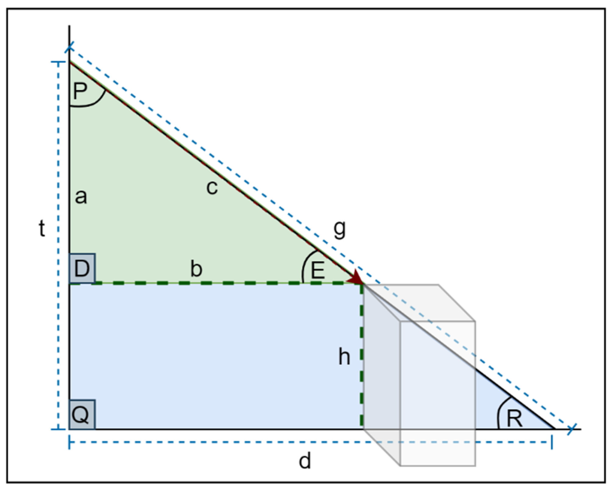
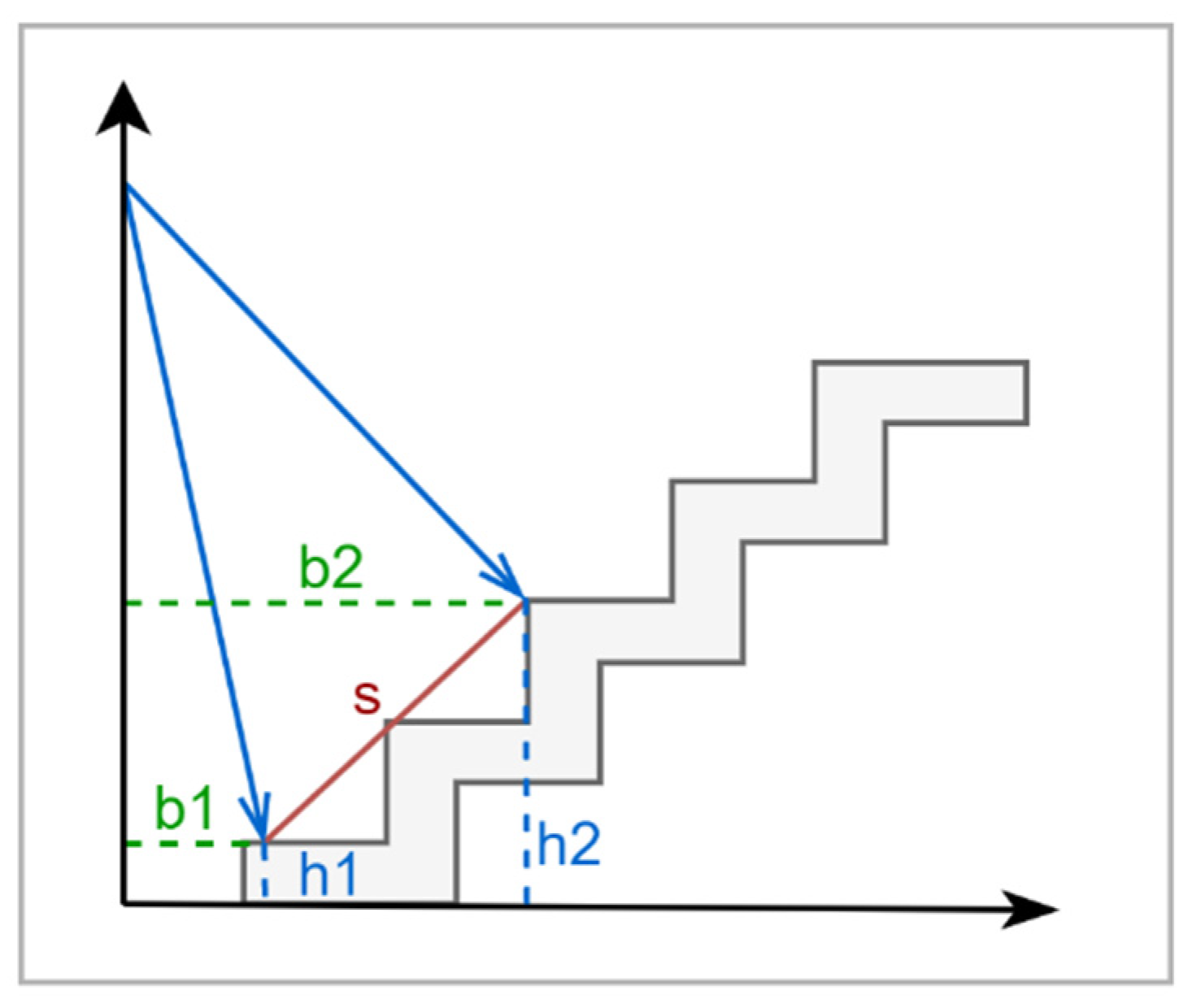
| PF2 | PF1 Extract 11 angle reading by dividing the 60 readings by 10 + angle no. 60 Add three features: Calculate the height of the obstacle of the starting angle of the LidSonic V2.0 device (angle closest to the user h1) Calculate the height of the obstacle of the middle angle of the LidSonic V2.0 device scan (h2) Calculate the slope between h1 and h2 |
| Obstacle Type | Data |
|---|---|
| DS1 Labels | a01, a02, a03, a04, a05, a06, a07, a08, a09, a10, a11, a12, a13, a14, a15, a16, a17, a18, a19, a20, a21, a22, a23, a24, a25, a26, a27, a28, a29, a30, a31, a32, a33, a34, a35, a36, a37, a38, a39, a40, a41, a42, a43, a44, a45, a46, a47, a48, a49, a50, a51, a52, a53, a54, a55, a56, a57, a58, a59, a60, Obstacle_class |
| Floor | 309, 305, 301, 295, 288, 285, 274, 266, 264, 260, 259, 253, 249, 243, 240, 229, 227, 211, 215, 214, 211, 208, 208, 205, 205, 197, 193, 191, 187, 186, 180, 176, 172, 169, 167, 172, 173, 172, 171, 169, 168, 167, 166, 165, 164, 163, 161, 161, 159, 158, 33, 25, 24, 23, 23, 26, 29, 120, 154, 157, 0 |
| Ascending Stairs | 141, 143, 143, 142, 143, 127, 145, 145, 142, 143, 144, 146, 147, 145, 141, 129, 133, 134, 127, 130, 134, 135, 135, 134, 134, 134, 134, 133, 131, 130, 128, 127, 124, 123, 122, 121, 119, 118, 119, 121, 130, 130, 129, 129, 128, 128, 124, 123, 124, 123, 123, 123, 122, 122, 132, 133, 132, 131, 133, 133, 1 |
| Descending Stairs | 696, 740, 841, 834, 575, 372, 380, 396, 608, 659, 654, 614, 546, 353, 343, 386, 389, 385, 382, 374, 359, 356, 355, 354, 350, 342, 336, 321, 308, 305, 303, 299, 296, 268, 264, 264, 262, 264, 263, 261, 254, 190, 189, 201, 215, 217, 211, 211, 209, 207, 208, 208, 206, 200, 154, 186, 186, 186, 185, 183, 2 |
| Wall | 49, 52, 46, 46, 46, 50, 51, 50, 52, 49, 53, 52, 50, 50, 55, 54, 57, 55, 55, 57, 58, 56, 57, 58, 62, 62, 62, 63, 65, 64, 66, 66, 69, 70, 78, 80, 83, 83, 84, 86, 88, 93, 95, 96, 102, 111, 123, 126, 118, 120, 120, 120, 122, 125, 129, 141, 152, 152, 152, 152, 3 |
| Deep Hole | 638, 643, 646, 650, 654, 659, 654, 661, 669, 663, 666, 668, 669, 672, 638, 631, 628, 630, 592, 588, 589, 592, 577, 554, 555, 532, 531, 531, 530, 528, 523, 520, 495, 494, 490, 487, 485, 482, 480, 476, 472, 450, 441, 443, 446, 438, 434, 434, 434, 436, 436, 430, 429, 427, 426, 423, 422, 422, 422, 421, 4 |
| High Obstacle | 87, 85, 85, 85, 85, 84, 84, 85, 89, 88, 91, 93, 93, 94, 99, 99, 100, 100, 98, 98, 98, 100, 100, 102, 103, 103, 103, 103, 102, 101, 99, 98, 96, 96, 95, 94, 93, 92, 91, 91, 91, 90, 88, 85, 86, 86, 84, 80, 78, 77, 77, 81, 81, 81, 81, 81, 81, 79, 78, 75, 5 |
| Bump | 237, 225, 217, 231, 239, 242, 227, 219, 219, 220, 228, 205, 205, 207, 210, 212, 212, 200, 196, 196, 196, 195, 194, 183, 184, 176, 174, 173, 170, 168, 167, 166, 164, 163, 160, 159, 158, 157, 153, 151, 151, 147, 144, 144, 144, 148, 148, 148, 147, 144, 143, 143, 143, 143, 143, 143, 142, 141, 140, 139, 6 |
| Hole | 275, 275, 298, 298, 273, 276, 284, 294, 296, 263, 254, 260, 262, 262, 254, 252, 252, 251, 249, 248, 245, 243, 231, 227, 228, 215, 214, 212, 212, 210, 209, 206, 203, 201, 201, 201, 200, 196, 189, 191, 191, 186, 184, 184, 185, 180, 181, 177, 178, 177, 178, 175, 173, 174, 174, 175, 174, 172, 171, 171, 7 |
| Obstacle Type | Data |
|---|---|
| DS2 Labels | a01, a06, a12, a18, a24, a30, a36, a42, a48, a54, a60, h1, h2, s, Obstacle_class |
| Floor | 309, 285, 253, 211, 205, 186, 172, 167, 161, 23, 157, 0.96, 2.42, 0.02, 0 |
| Ascending Stairs | 141, 127, 146, 134, 134, 130, 121, 130, 123, 122, 133, 24.21, 47.76, 0.54, 1 |
| Descending Stairs | 696, 372, 614, 385, 354, 305, 264, 190, 211, 200, 183, −24.20, −93.90, −0.55, 2 |
| Wall | 49, 50, 52, 55, 58, 64, 80, 93, 126, 125, 152, 5.81, 101.19, 19.06, 3 |
| Deep Hole | 638, 659, 668, 630, 554, 528, 487, 450, 434, 427, 421, −254.67, −274.42, −0.09, 4 |
| High Obstacle | 87, 84, 93, 100, 102, 101, 94, 90, 80, 81, 75, 80.37, 71.23, −0.23, 5 |
| Bump | 236, 264, 221, 209, 182, 173, 162, 152, 148, 141, 139, 18.39, 12.95, −0.08, 6 |
| Hole | 275, 276, 260, 251, 227, 210, 201, 186, 177, 174, 171, −12.58, −17.0, −0.05, 7 |
| Dataset | TModel1 | TModel2 |
|---|---|---|
| Training feature shape | (435, 60) | (435, 14) |
| Validation feature shape | (109, 60) | (109, 14) |
| Test feature shape | (136, 60) | (136, 14) |
| Model: “Sequential_16” | ||
|---|---|---|
| Layer (Type) | Output Shape | Parameters |
| flatten_16 (Flatten) | (None, 60) | 0 |
| dense_74 (Dense) | (None, 60) | 3660 |
| dense_75 (Dense) | (None, 120) | 7320 |
| dense_76 (Dense) | (None, 60) | 7260 |
| dense_77 (Dense) | (None, 60) | 3660 |
| dense_78 (Dense) | (None, 30) | 1830 |
| dense_79 (Dense) | (None, 8) | 248 |
| Total params: 23,978 | ||
| Trainable params: 23,978 | ||
| Non-trainable params: 0 | ||
| Model: “Sequential_2” | ||
|---|---|---|
| Layer (Type) | Output Shape | Parameters |
| flatten_2 (Flatten) | (None, 14) | 0 |
| dense_8 (Dense) | (None, 140) | 2100 |
| dense_9 (Dense) | (None, 64) | 9024 |
| dense_10 (Dense) | (None, 30) | 1950 |
| dense_11 (Dense) | (None, 8) | 248 |
| Total params: 13,322 | ||
| Trainable params: 13,322 | ||
| Non-trainable params: 0 | ||
| Specifications | Value |
|---|---|
| Number of hidden layers—Tmodel1 | 5 |
| Number of hidden layers—Tmodel2 | 3 |
| Activation function—hidden layers | Relu |
| Activation function—output layer | Softmax |
| Loss function categorical | Sparse_categorical_crossentropy |
| Optimizer | Adam |
| Epochs | 200 |
| Trained Model | Dataset | No. of Features | Classifier | Precision | Accuracy |
|---|---|---|---|---|---|
| IBk-DS1 | DS1 | 60 | IBk | 94.0 | 93.68 |
| RC-DS1 | DS1 | 60 | Random Committee | 94.7 | 94.56 |
| KStar-DS1 | DS1 | 60 | KStar | 95.6 | 95.44 |
| IBk-DS2 | DS2 | 14 | IBk | 95.2 | 95 |
| RC-DS2 | DS2 | 14 | Random Committee | 95.2 | 95.15 |
| KStar-DS2 | DS2 | 14 | KStar | 94.1 | 93.82 |
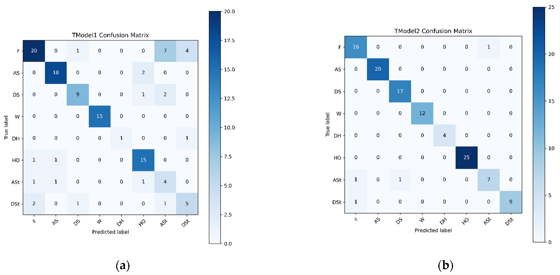
| Class | Abbreviation | Class | Abbreviation |
|---|---|---|---|
| Floor | F | Deep Hole | DH |
| Ascending Stairs | AS | High Obstacle | HO |
| Descending Stairs | DS | Ascending Step | Ast |
| Wall | W | Descending Step | DSt |
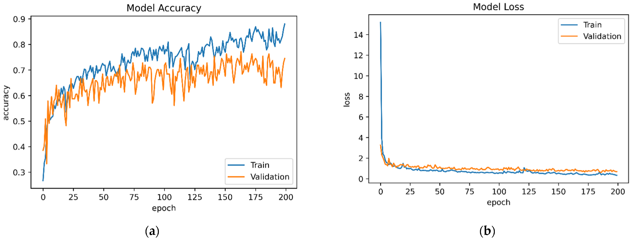
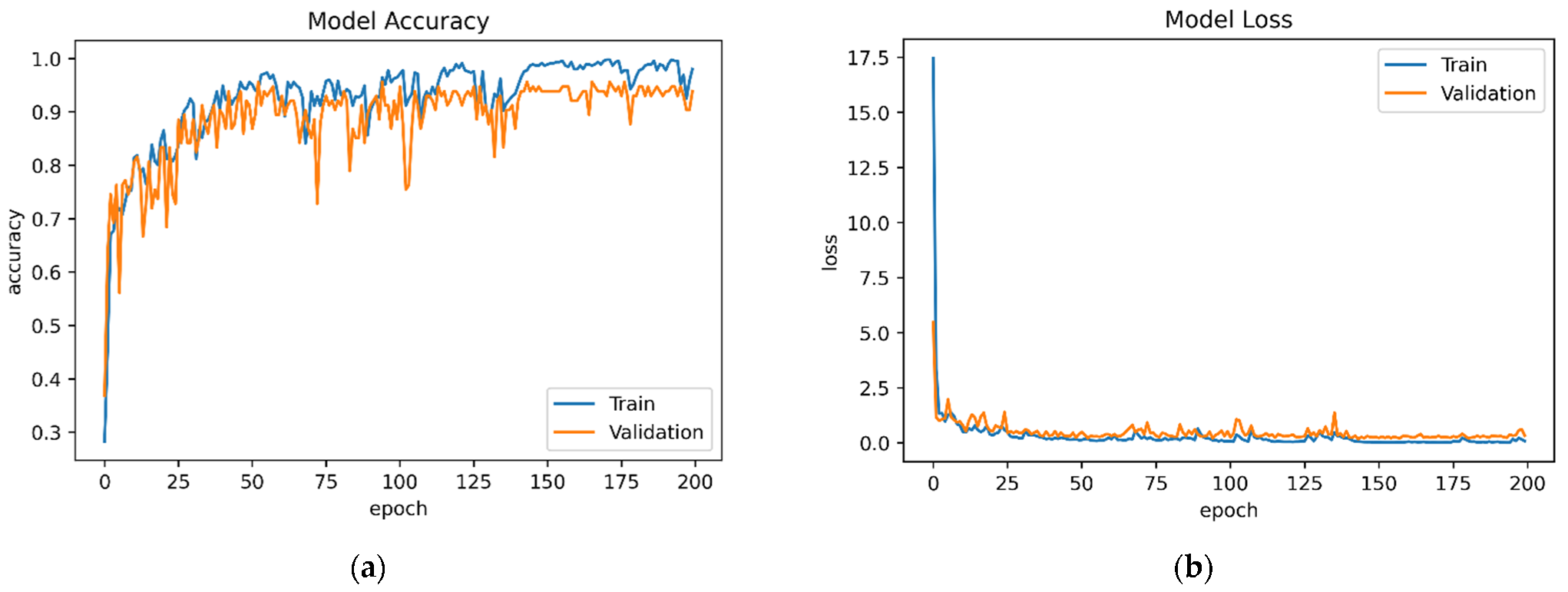
| Trained Model | Dataset | Features | Model Accuracy | Test Accuracy | Model Loss | Test Loss |
|---|---|---|---|---|---|---|
| TModel1 | D1 | 60 | 88.05 | 76.32 | 0.3374 | 0.7190 |
| TModel2 | D2 | 14 | 98.01 | 96.49 | 0.0883 | 0.3672 |
Publisher’s Note: MDPI stays neutral with regard to jurisdictional claims in published maps and institutional affiliations. |
© 2022 by the authors. Licensee MDPI, Basel, Switzerland. This article is an open access article distributed under the terms and conditions of the Creative Commons Attribution (CC BY) license (https://creativecommons.org/licenses/by/4.0/).
Share and Cite
Busaeed, S.; Katib, I.; Albeshri, A.; Corchado, J.M.; Yigitcanlar, T.; Mehmood, R. LidSonic V2.0: A LiDAR and Deep-Learning-Based Green Assistive Edge Device to Enhance Mobility for the Visually Impaired. Sensors 2022, 22, 7435. https://doi.org/10.3390/s22197435
Busaeed S, Katib I, Albeshri A, Corchado JM, Yigitcanlar T, Mehmood R. LidSonic V2.0: A LiDAR and Deep-Learning-Based Green Assistive Edge Device to Enhance Mobility for the Visually Impaired. Sensors. 2022; 22(19):7435. https://doi.org/10.3390/s22197435
Chicago/Turabian StyleBusaeed, Sahar, Iyad Katib, Aiiad Albeshri, Juan M. Corchado, Tan Yigitcanlar, and Rashid Mehmood. 2022. "LidSonic V2.0: A LiDAR and Deep-Learning-Based Green Assistive Edge Device to Enhance Mobility for the Visually Impaired" Sensors 22, no. 19: 7435. https://doi.org/10.3390/s22197435
APA StyleBusaeed, S., Katib, I., Albeshri, A., Corchado, J. M., Yigitcanlar, T., & Mehmood, R. (2022). LidSonic V2.0: A LiDAR and Deep-Learning-Based Green Assistive Edge Device to Enhance Mobility for the Visually Impaired. Sensors, 22(19), 7435. https://doi.org/10.3390/s22197435