
UAV and IoT-Based Systems for the Monitoring of Industrial Facilities Using Digital Twins: Methodology, Reliability Models, and Application


 , ,
, ,  ,
, 
Abstract
:1. Introduction and Related Works
1.1. Motivation
- There are a large number of emergency facilities, enterprises, and transport and energy systems that are part of regional, national, and even transnational infrastructures. Thus, their influence grows not only on the continuous and high-quality provision of relevant products, resources, and services, but also on the potential danger of certain territories and regions (more and more dangerous objects) [1,2].
- These systems are becoming more robotic and lacking in human participation, considering the trends in the development and implementation of the principles of Industry 4.0 [3,4]. As a result, monitoring systems need to develop appropriately, based on digital, mobile, and smart technologies; this is necessary to effectively perform control and monitoring functions on equipment and the surrounding areas; or environmental monitoring tasks, including possible pollution, forest resources, and fires (more and more robotic unmanned industries); and develop facilities for environmental monitoring (forest fires, etc.) [5,6].
- New technologies (Internet of Things (IoT) and Internet of Everything, big data analytics, digital twins (DTs) and X-reality, and unmanned aerial vehicles (UAVs), commonly known as drones, robotics, etc.) create new opportunities for the creation of monitoring systems; however, they are the cause of challenges related to dependability, functional safety, and cybersecurity components and monitoring systems, which operate in very harsh physical and informational conditions [7,8,9].
1.2. State of the Art
- Monitoring system dependability studies, considering the possible degradation of systems due to channel failures and the corresponding reduction in the “monitoring coverage” of industrial facilities and their surrounding areas. In this case, it is advisable to use models of multi-state systems (MSSs) [75].
1.3. Objectives
- To develop a methodology for building and creating general models (structures) of UAV-, IoT-, and DT-based monitoring systems in complex industrial facilities as multi-level and multi-state systems;
- To develop and explore reliability models of the monitoring systems considering applied mobile and digital technologies, operation modes (normal and emergency), etc.;
- To propose and discuss industrial cases of monitoring systems for manufacturing and nuclear power plants.
1.4. Approach and Structure
- Parts of critical infrastructures such as nuclear power plant utilities, dangerous manufacturers, oil and gas transport communications, etc.
- Described using a multilevel hierarchy scheme, and based on the application of the technologies:
- (a)
- Digital twins as models of controlled sub-objects;
- (b)
- UAV fleet as an additional channel for collecting information;
- (c)
- A private cloud system as a redundant emergency center for decision-making support.
- Various monitoring system structures, options for sub-object monitoring, and the configuration of different stationary and mobile centers for collecting information and decision making;
- Modes of monitoring system operation (normal and emergency modes) that vary in terms of the environment and failure rates of the components;
- The placement and reliability of digital twins generated by different centers and their influence on decision making;
- The placement and reliability of decision-making units;
- The processes of monitoring system degradation caused by components and channels failures. In this case, the monitoring system is addressed as an MSS.
2. Methodology for Building SMs
2.1. Concept of SM Building
2.2. Principles of SM Building
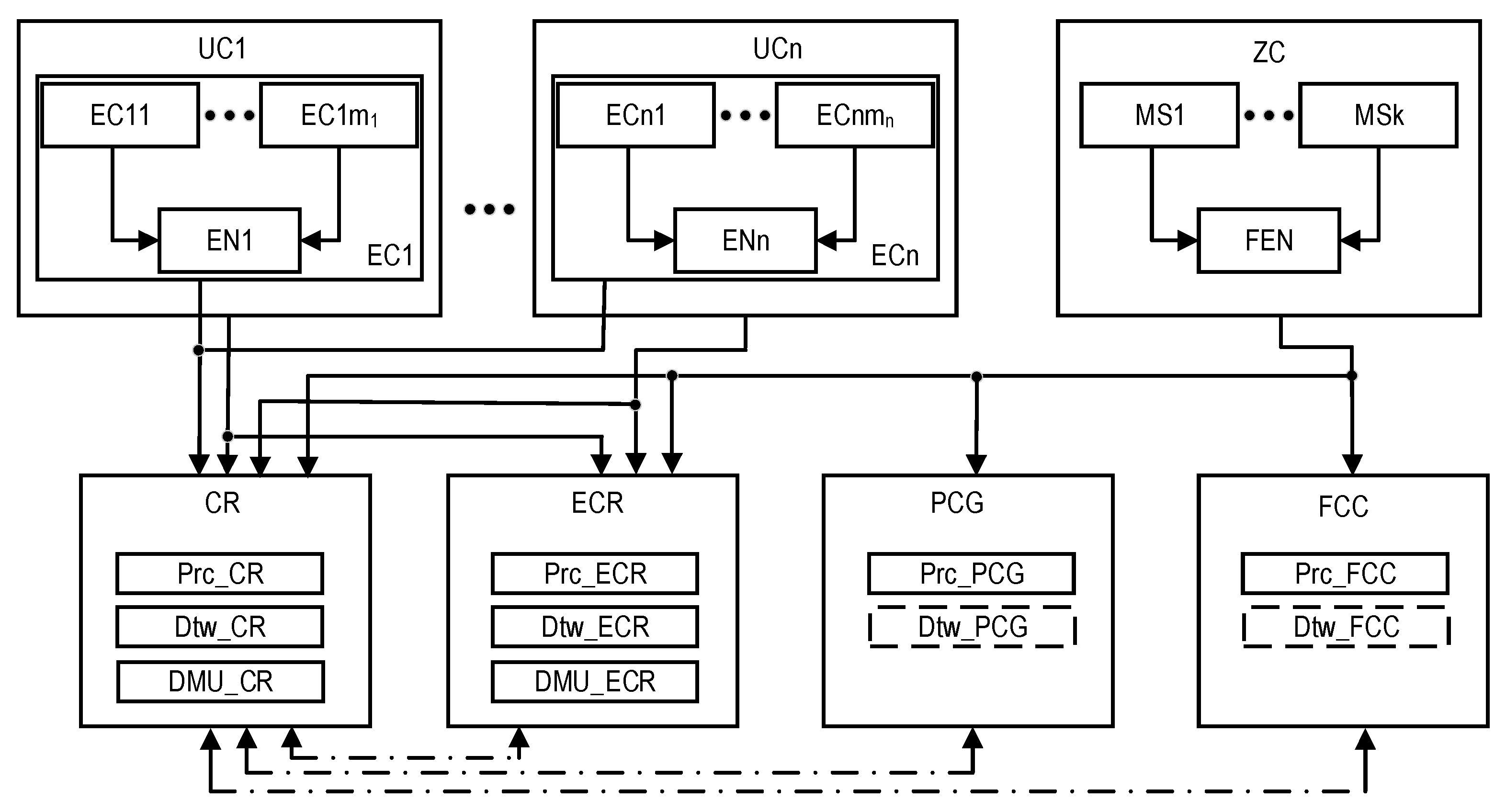
2.2.1. Three-Level Model of Object Monitoring
- Equipment with sensors and critical-process management devices (equipment that is monitored and controlled, EC). Various systems of such monitoring are used in industrial facilities. They are based on wireless and IoT technologies and do not interfere with technological processes, without creating additional risks from the point of view of ensuring the safety of objects.
- Several systems and building complexes, within which equipment with sensors and devices for the management of critical processes (the utility that is monitored and controlled, UC) were placed. For example, for a nuclear power plant, this level covers systems and equipment whose condition is monitored by the Post-Accident Monitoring System [76].
- The territory of the industrial facility, which is limited by the outer perimeter, where monitoring stations (MSs) are located (zones that are monitored, ZC). For a nuclear power plant, this corresponds to the area whose condition is monitored by the Automated Radiation Monitoring System [77].
2.2.2. Applied Technologies
- DTs, which ensure the creation of digital clones in an industrial facility. This makes it possible to model and determine its state from various data on the state of its component systems and objects. The creation and use of DTs of different complexity for different crisis centers are envisaged. The model uses a digital twin instance which describes a specific object with which the twin remains associated through the life of the object. Duplicates of this type usually contain an annotated 3D model, which takes into account the measurement results received from the sensors, as well as the current and predicted values of the monitoring parameters.
- IoT and Internet of Flying Things to reserve wired data transmission channels from sensors and critical-process control devices, commonly equipped with previous-generation Post-Accident Monitoring Systems and Automated Radiation Monitoring Systems. Post-Accident Monitoring Systems were created in the first decade after the Fukushima accident [76,77].
- Edge computing technologies for data pre-processing at every level of the industrial facility monitoring model using edge nodes (EN), which make it possible to reduce data volumes, their transmission speed, and the requirements for the performance of transmission equipment. Data pre-processing also increases the efficiency of decision-making processing in crisis centers. The model of the monitoring system aims to perform boundary calculations and the placement of relevant edge nodes on both UCs and onboard UAVs (flying edge nodes, FENs).
2.2.3. Redundant Centers of Control and Monitoring
- The private cloud crisis group (PCG), which processes monitoring data using cloud services and the Internet of Things;
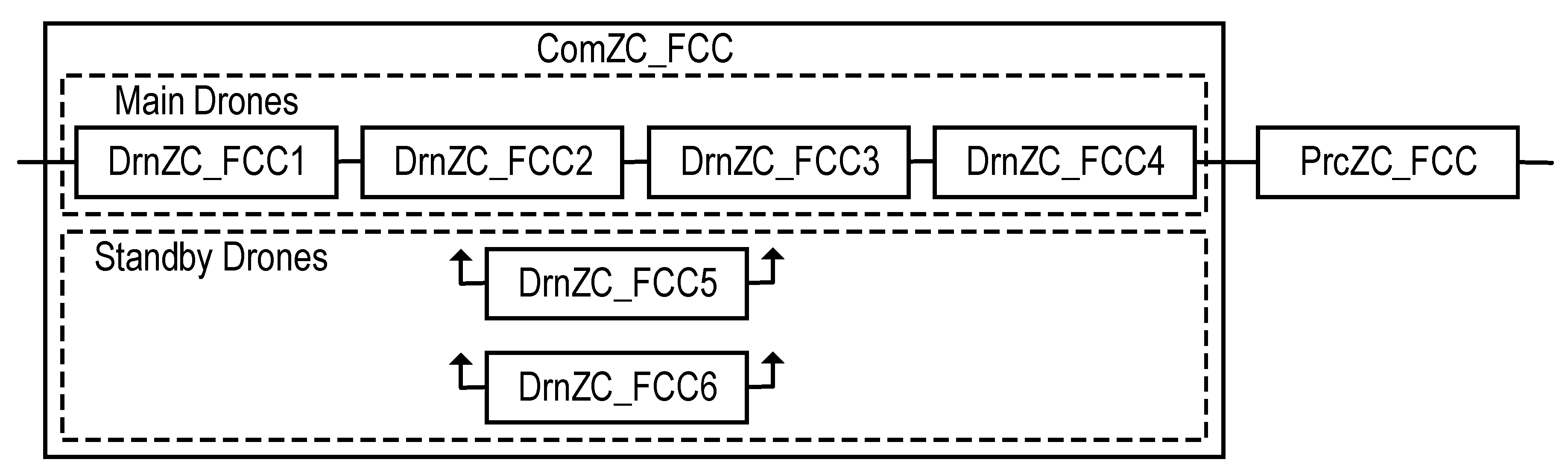
- The UAV Fleet and flying control center (FCC), which receive and processes data on the condition of an industrial facility using equipment that can be placed either on one powerful UAV or under a group of UAVs (UAV fleet or IoD), can be distributed. The IoD is a kind of Internet of Flying Things based on a set of interacting drones. For the considered SMs, the IoD is a part of the flying control center (FCC) infrastructure with access to both the Private Cloud and Internet resources. Drone on-board systems collaborate with each other, ground sensors (located at the MSs), and the FCC.
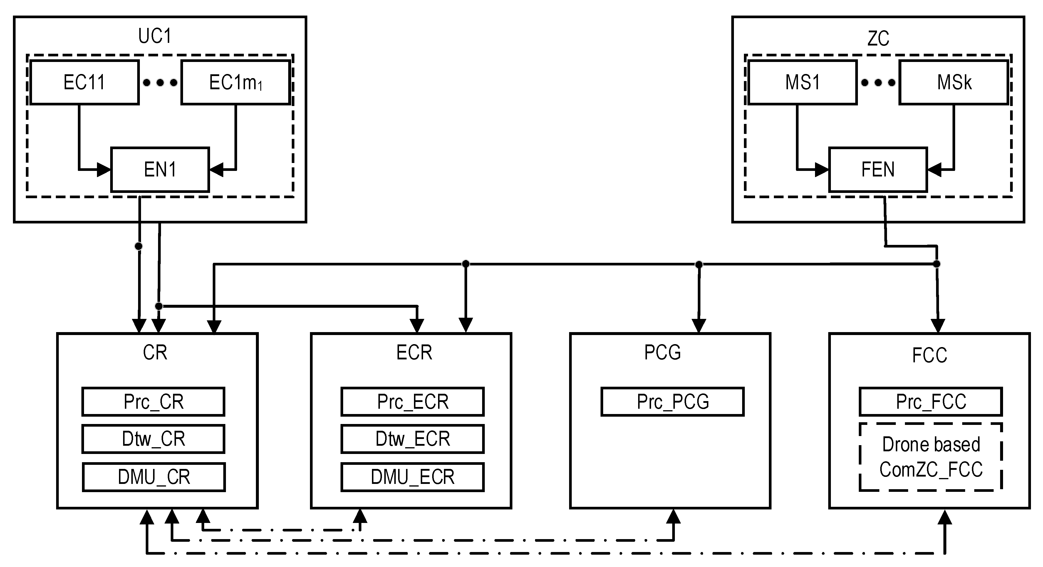
2.2.4. General Model of the Industrial Facility Monitoring System
2.3. Structures of SMs

3. Reliability Models for System of Monitoring
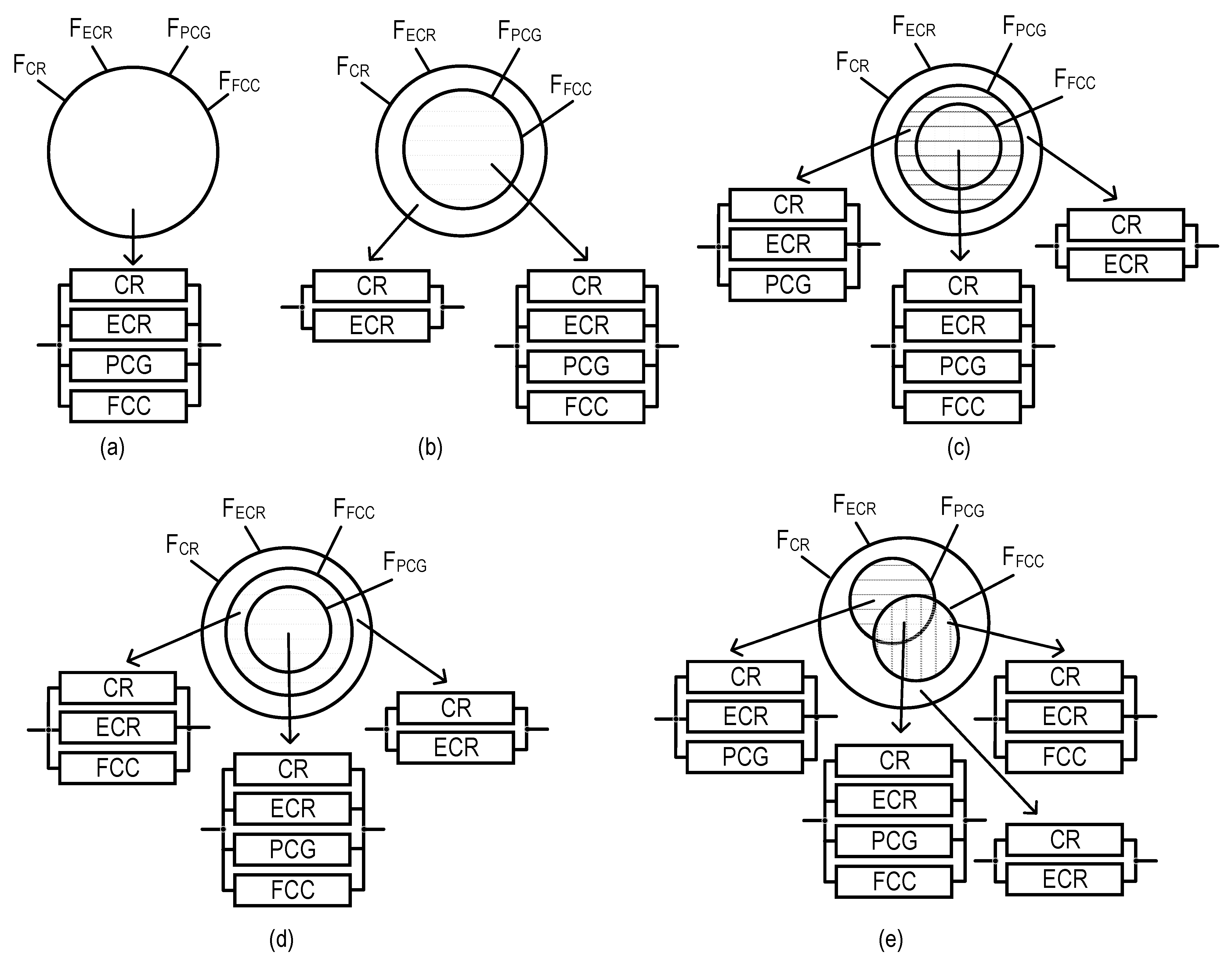
3.1. Models of SM Option Field-Monitoring Coverage
- For the EC, the DTs are formed only in CR, so there is no compatibility problem here.
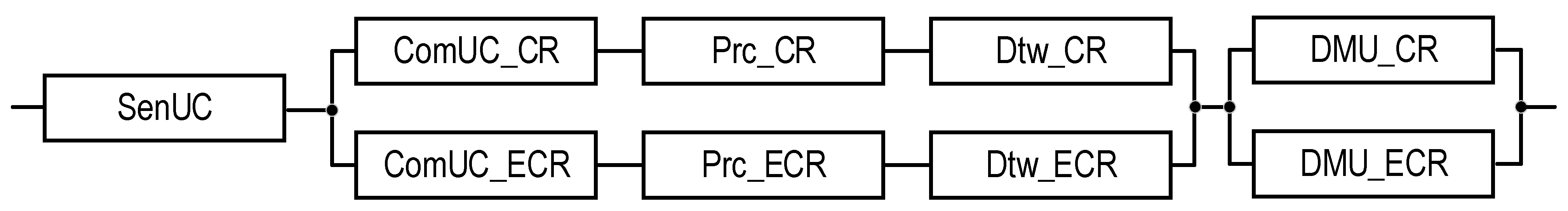
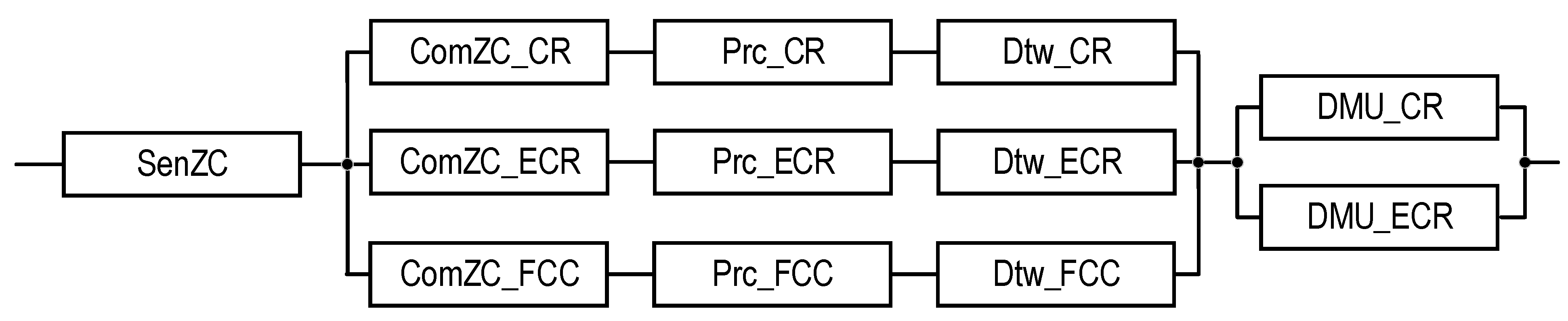
- For UC, DTs are formed in CR and ECR from common sensors, so the data for generating DTs are identical, and, therefore, their compatibility is ensured. In addition, these data are corrected by the DMU in cases of failure.
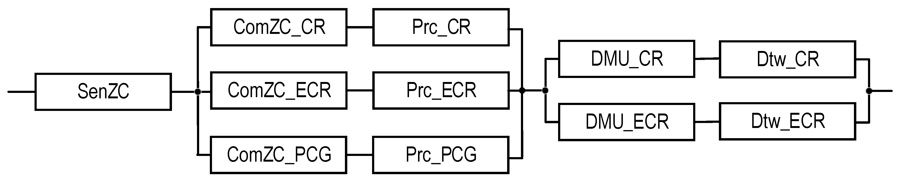
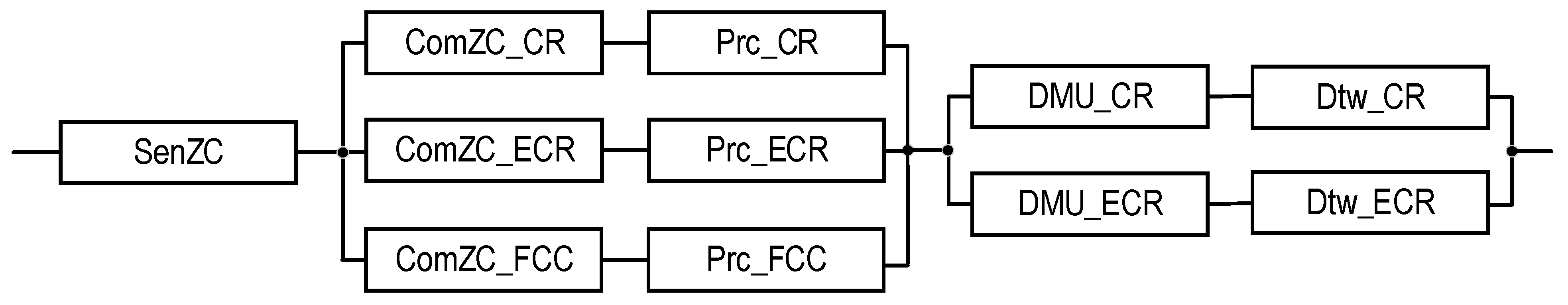
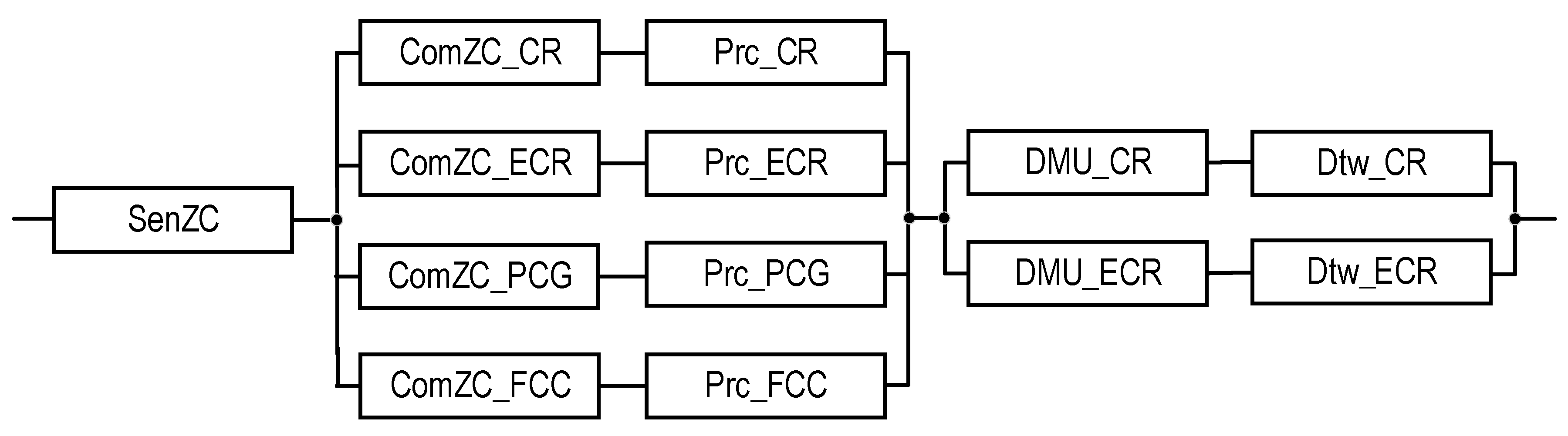
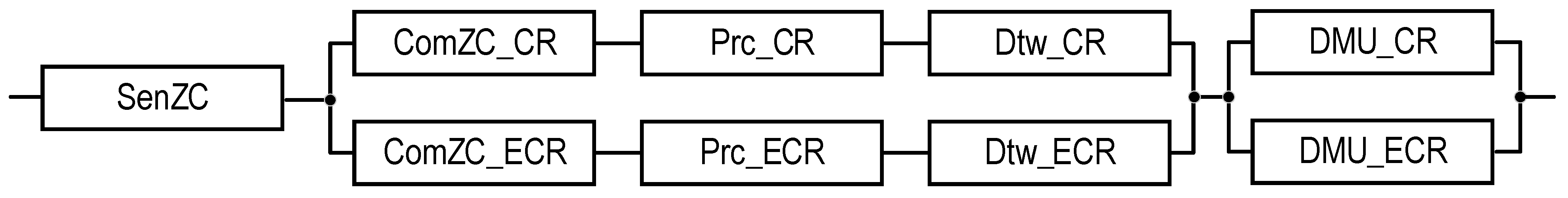
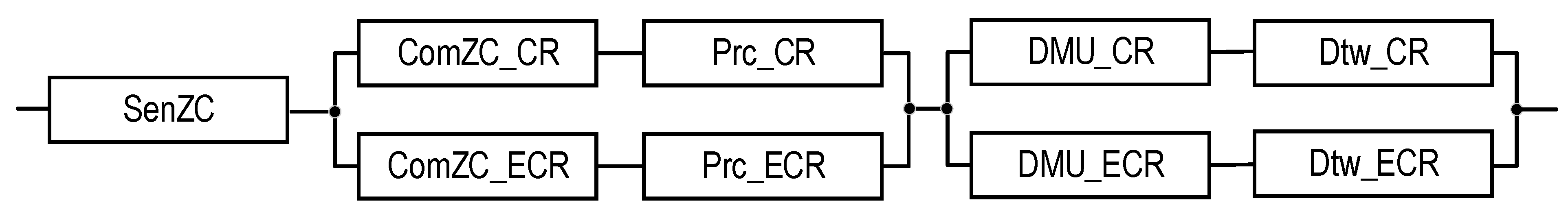
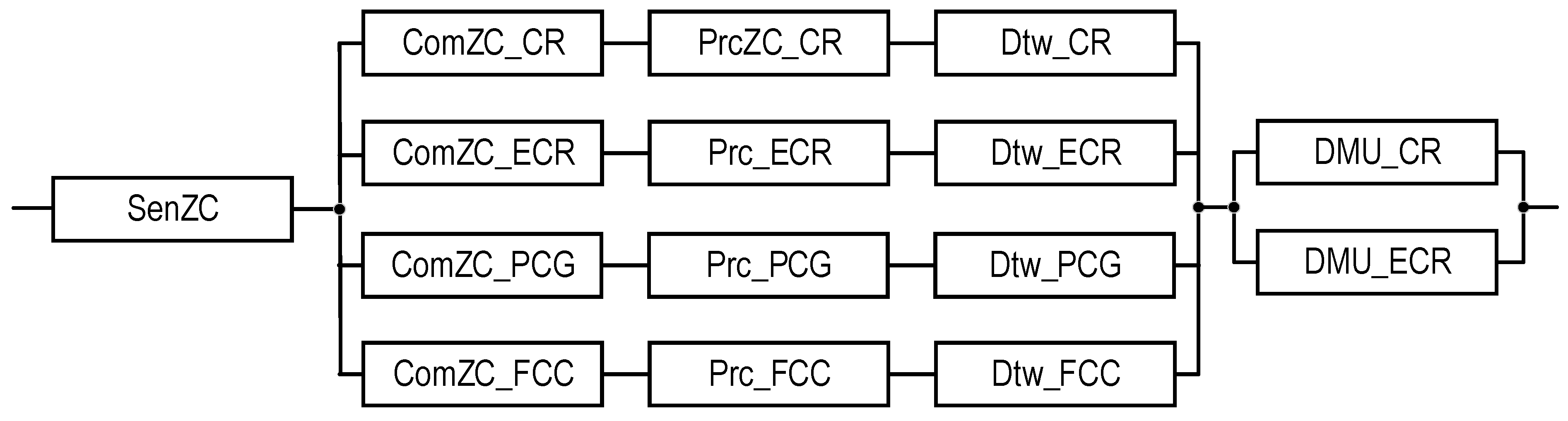
- For ZC, DTs are formed by all the subsystems (CR, ECR, PCG, and FCC) from sensors located in the ZC zone. If all subsystems use the full amount of monitoring data, both the compatibility and reliability of DT formation are ensured as in the previous case, using the DMU. If PCG and FCC subsystems use a limited data set from sensors, these data are employed to form the corresponding part of DTs and combine it with data from CR and ECR to ensure the DT’s compatibility.
- Channels can perform the same set of monitoring functions;
- The set of monitoring functions for some channels can be considered as a subset of monitoring functions for other channels;
- Sets of monitoring functions for individual channels may overlap.
3.2. Extended Specification for SM Structures
- −
- The third channel for the three-channel SM structure (PCG or FCC);
- −
- The designation of the SM structure;
- −
- The reliability block diagram for the SM;
- −
- The notations of the SM structure and SM reliability function;
- −
- The equation for calculating the SM reliability function.

| Source of Information | Mode | Number of Channels | Type of Structure | Third Channel for Three-Channel SM structure | Notation of SM Structure | Reliability Block Diagram for SM | Notation of SM Reliability Function | Equation for Calculating SM Reliability Function |
|---|---|---|---|---|---|---|---|---|
| EC | Normal | 1 | T2 | - | Figure 3 | Equation (1) | ||
| EC | Emergency | 1 | T2 | - | Figure 3 | Equation (2) | ||
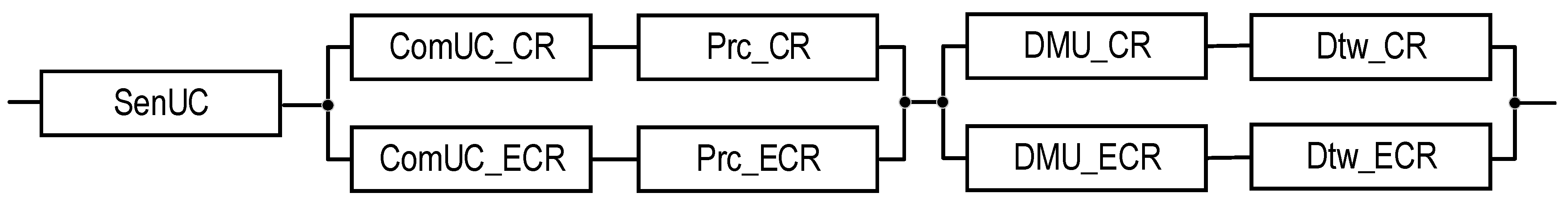
| UC | Normal | 2 | T1 | - | Figure 4 | Equation (3) | ||
| UC | Emergency | 2 | T1 | - | Figure 4 | Equation (4) | ||
| UC | Normal | 2 | T2 | - | Figure 5 | Equation (5) | ||
| UC | Emergency | 2 | T2 | - | Figure 5 | Equation (6) | ||
| ZC | Normal | 2 | T1 | - | Figure 6 | Equation (7) | ||
| ZC | Emergency | 2 | T1 | - | Figure 6 | Equation (8) | ||
| ZC | Normal | 2 | T2 | - | Figure 7 | Equation (9) | ||
| ZC | Emergency | 2 | T2 | - | Figure 7 | Equation (10) | ||
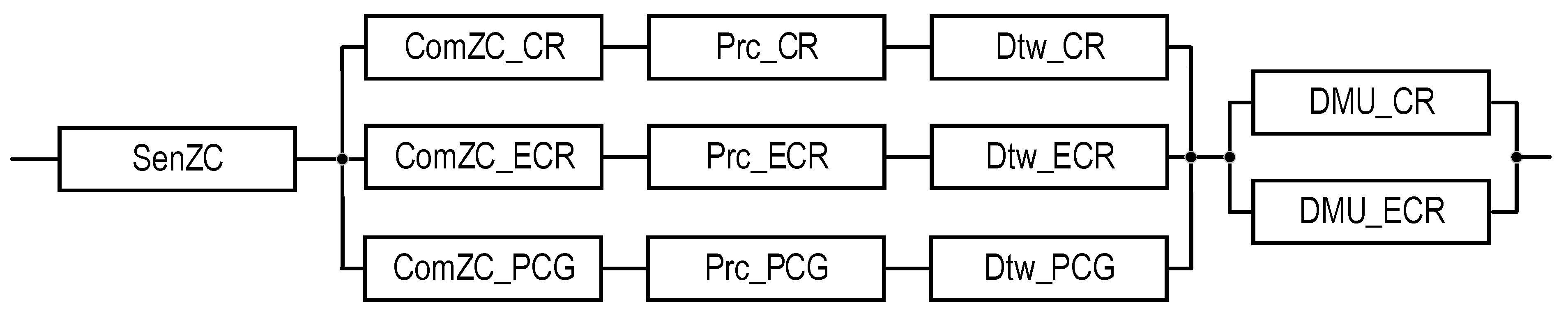
| ZC | Emergency | 3 | T1 | PCG | Figure 8 | Equation (11) | ||
| ZC | Emergency | 3 | T2 | PCG | Figure 9 | Equation (12) | ||
| ZC | Emergency | 3 | T1 | FCC | Figure 10 | Equation (13) | ||
| ZC | Emergency | 3 | T2 | FCC | Figure 11 | Equation (14) | ||
| ZC | Emergency | 4 | T1 | - | Figure 12 | Equation (15) | ||
| ZC | Emergency | 4 | T2 | - | Figure 13 | Equation (16) |
3.3. Reliability Models
3.3.1. Notations and Assumptions
- Components of the SM have an exponential time to failure;
- During the operating time, the SM is considered an unrecoverable system.
3.3.2. Description and Simulation of the Reliability Models


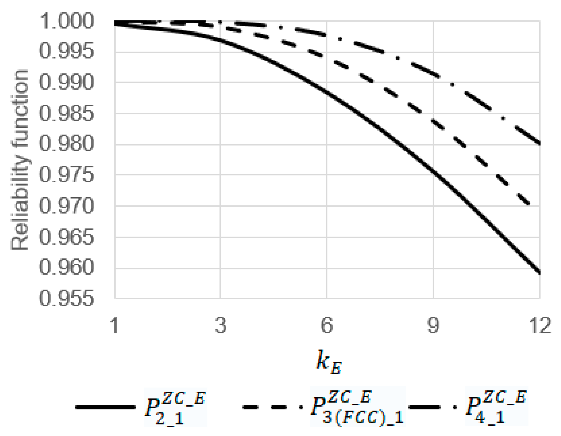

- At , the increase in the emergency coefficient from 1 to 12 leads to a decrease in the values of the reliability functions , , and 1.04 (from 0.99961 to 0.95921), 1.03 (from 0.99996 to 0.97409), and 1.02 (from 0.99999 to 0.98019) times, respectively (Figure 14);
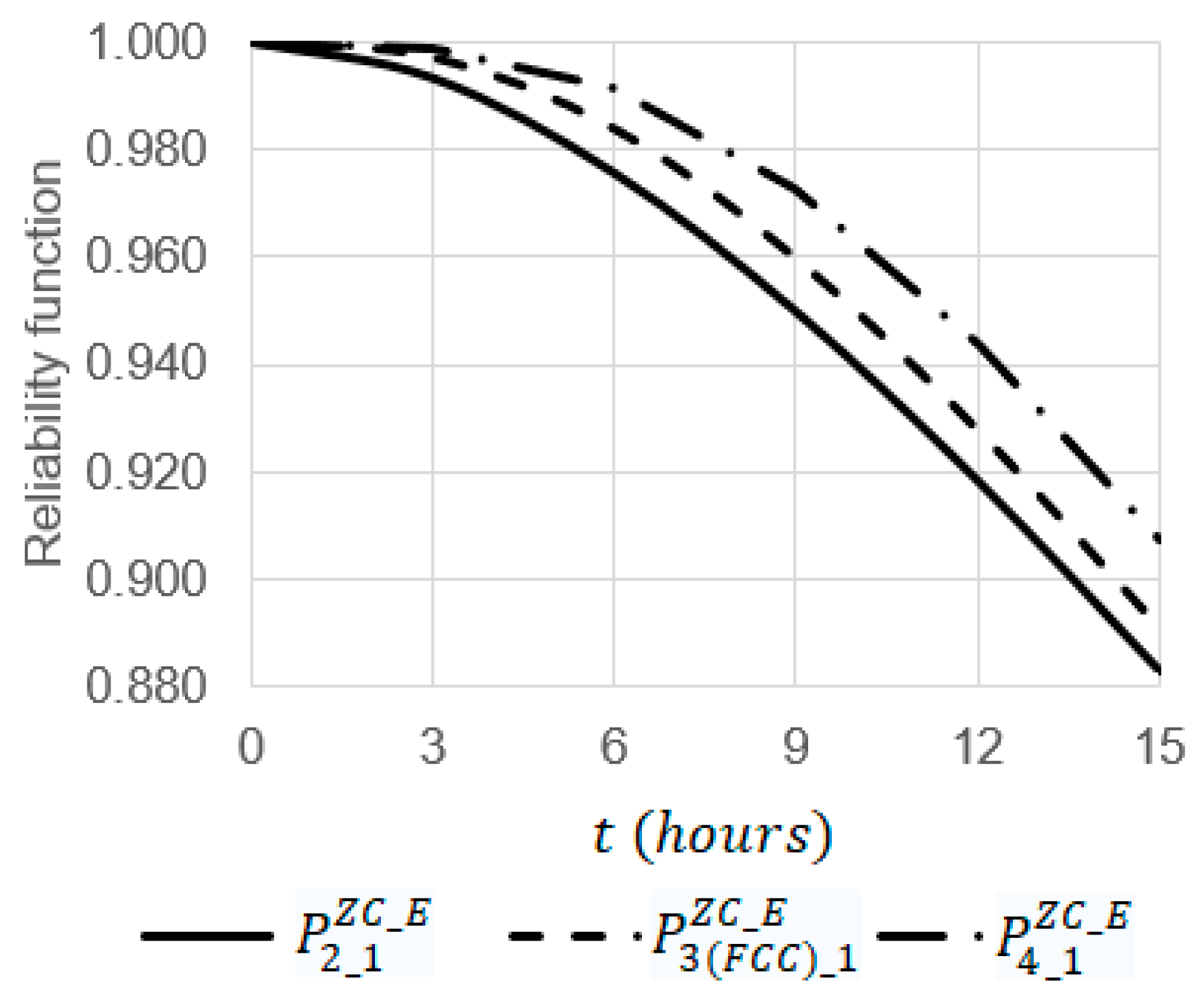
- At , the increase in the operating time from 0 to 15 leads to a decrease in the values of the reliability functions , , and 1.13 (from 1 to 0.88303), 1.12 (from 1 to 0.89077), and 1.1 (from 1 to 0.90725) times, respectively (Figure 15);
- Among the systems , , and , the most reliable system is and the most unreliable one is . For example, at and , the value of the reliability function is 1.02 times larger than the value of the reliability function (0.94358 against 0.92764) and 1.03 times larger than the value of the reliability function (0.94358 against 0.92764) (Figure 15).
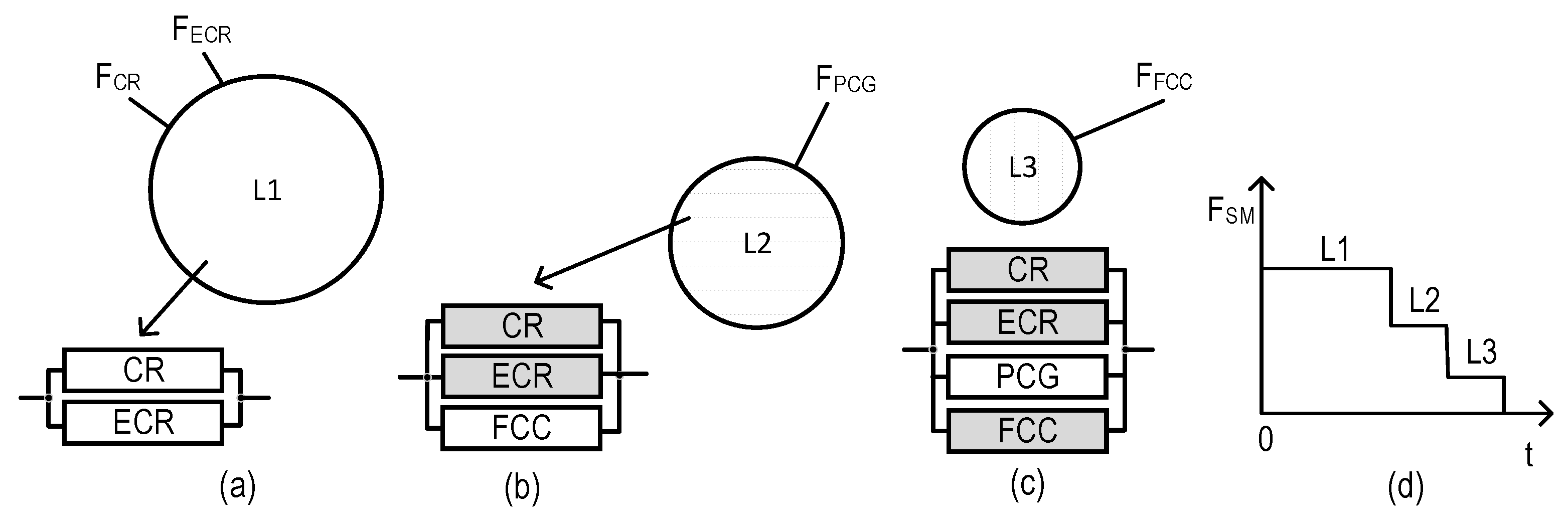
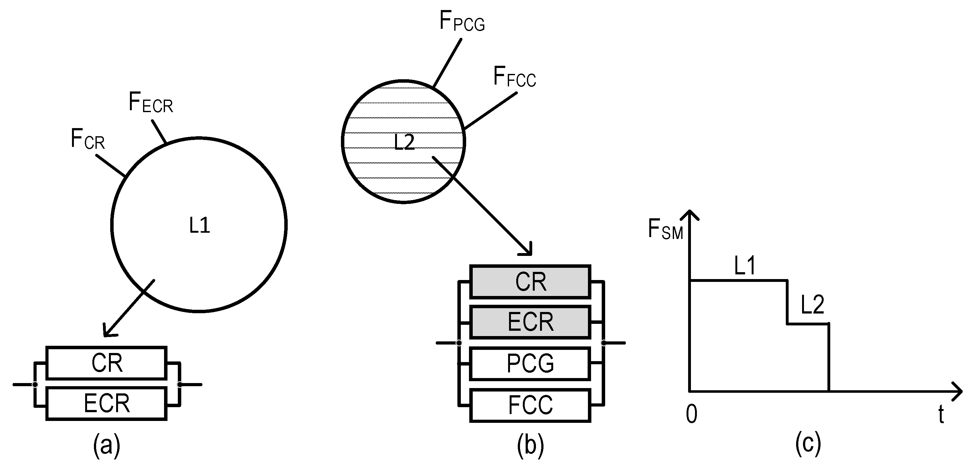
3.4. Models of SM as a Multi-State System
3.4.1. Description of SM as a Multi-State System


3.4.2. Reliability Models
3.4.3. Simulation and Analysis
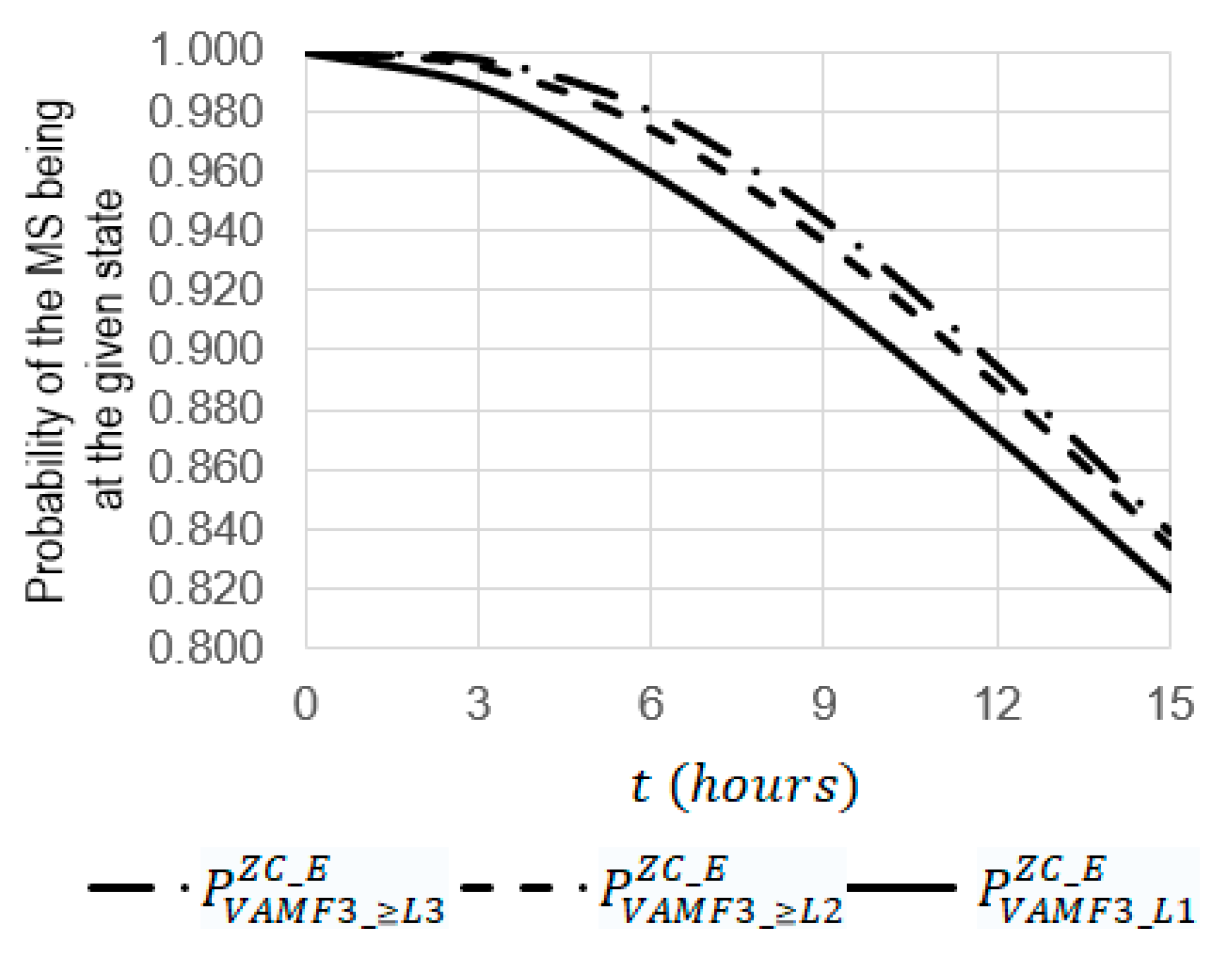
- The increase in the operating t time from 0 to 15 leads to a decrease in the probabilities of , , and by 1.19 (from 1 to 0.83865), 1.20 (from 1 to 0.83419), and 1.21 (from 1 to 0.81969), respectively;
- At , the probability of is 1.01 times larger than the probability of , (0.83865 against 0.93633) and 1.02 times larger than the probability of (0.83865 against 0.81969);
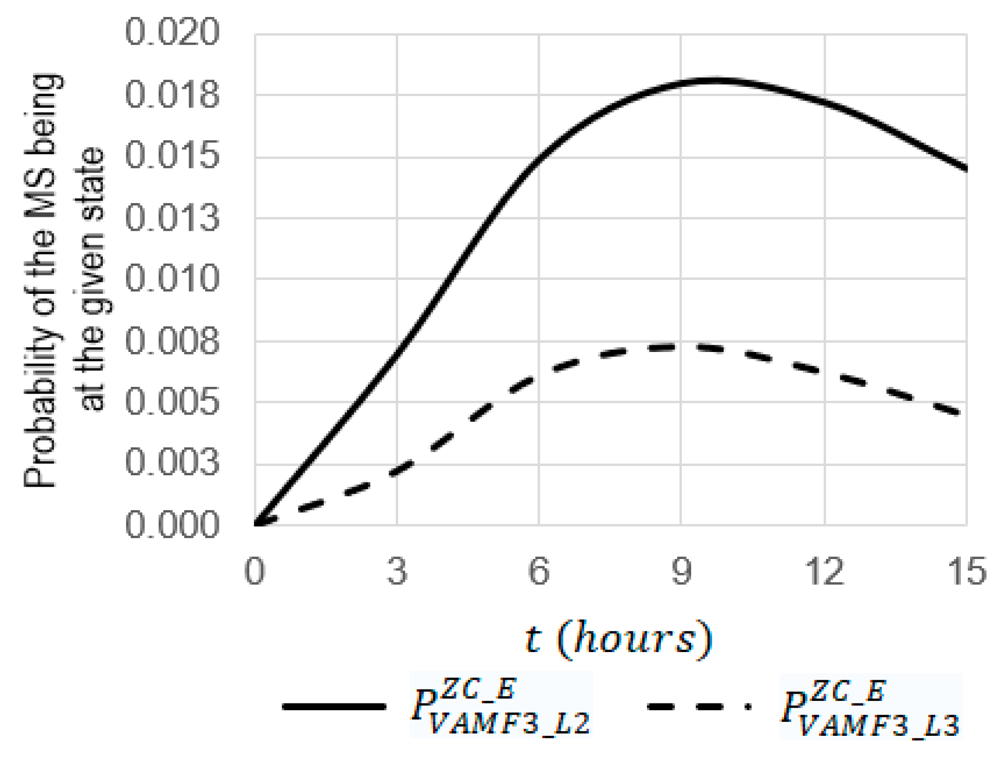
- At , the function of has a maximum equal to 0.185 and, at , the function has a maximum equal to 0.008.
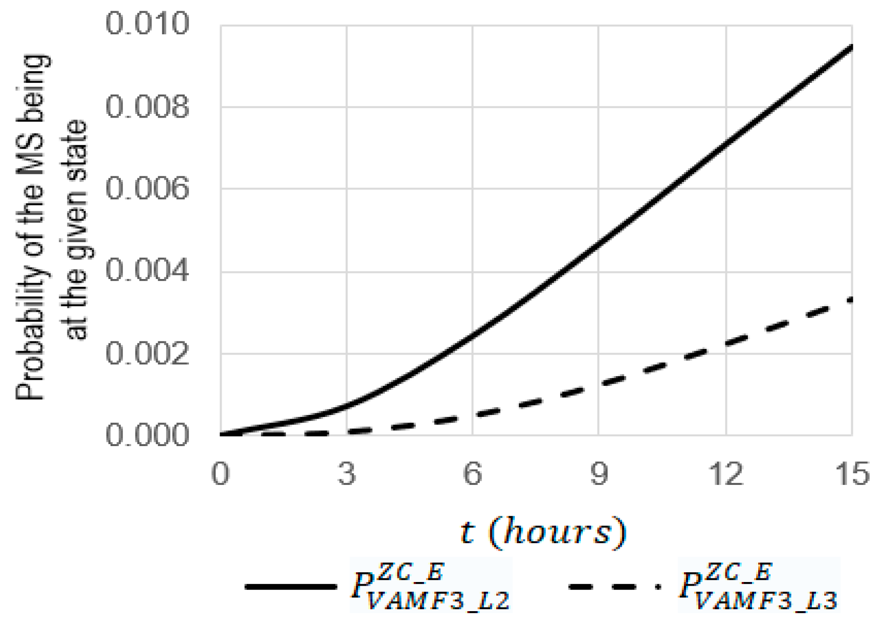
- The increase in the operating time from 0 to 15 leads to an increase in the probabilities of and from 0 to 0.00945 and from 0 to 0.00333, respectively;
- At , the probability of is 2.84 times larger than the probability of (0.00466 against 0.00124);
- At , the probability of is 3.77 times larger than the probability of (0.00945 against 0.00333).
4. Case Study
4.1. Drone Fleet and IoD-Based Industrial Facility Monitoring System
4.1.1. Structure of IoD SM
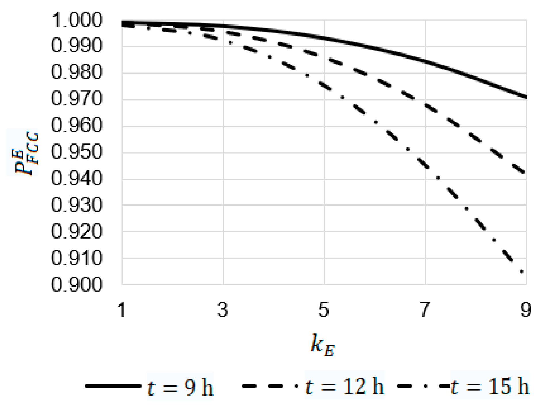
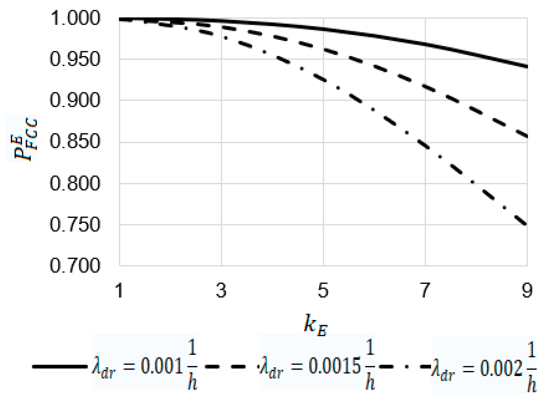
4.1.2. Reliability Model of FCC Channel
- At , , and the increase in the emergency coefficient from 1 to 9 leads to a decrease in the value of the reliability function from 0.99904 to 0.97100, from 0.99904 to 0.94181, and from 0.99824 to 0.90306, respectively;
- At the value of the reliability function at is 1.03 times larger than at (0.97100 against 0.94181) and 1.08 times larger than at (0.97100 against 0.90306).
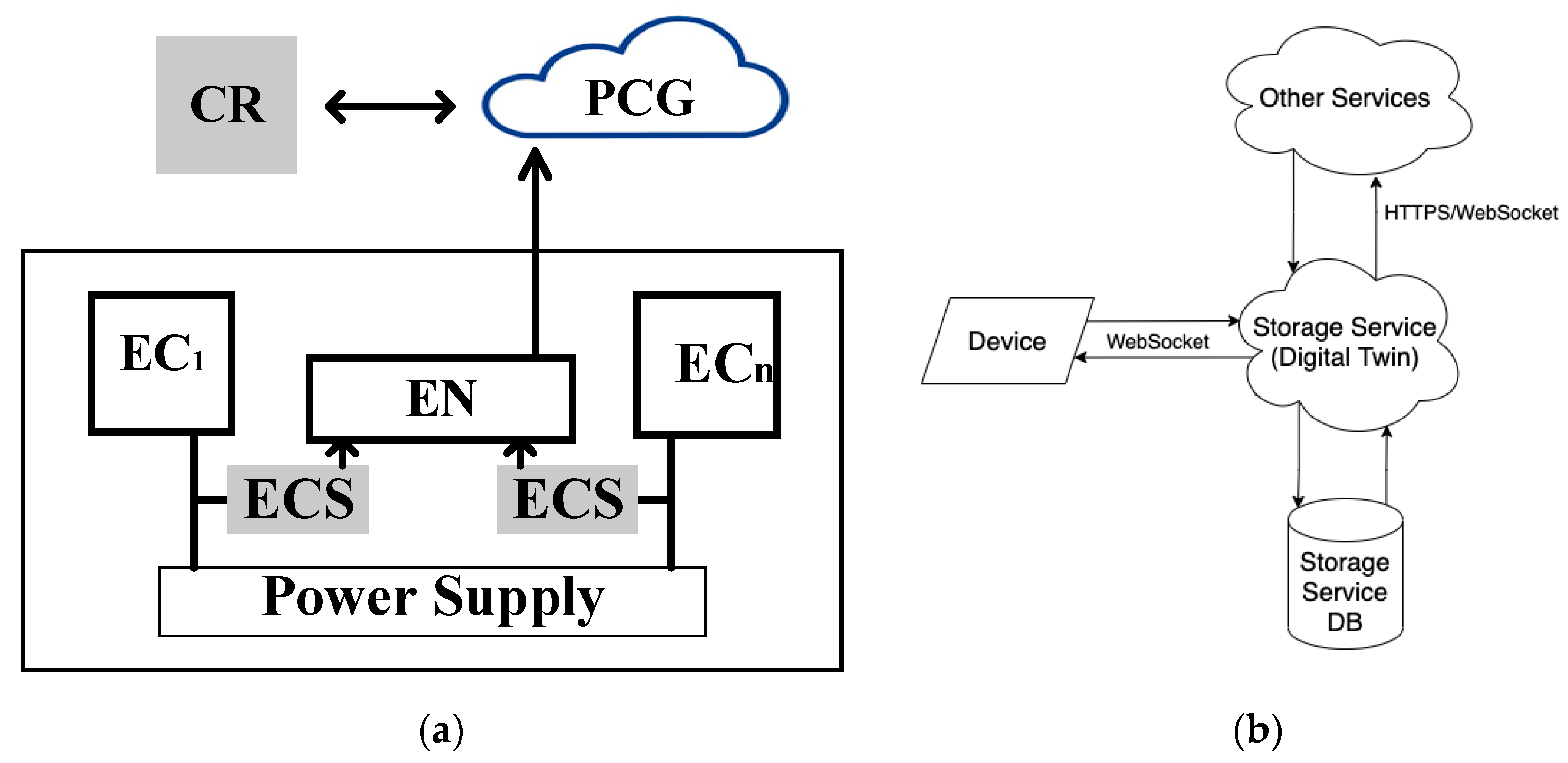
4.2. The Equipment Monitoring System
4.2.1. Principles and Structure
4.2.2. Processes and Algorithms of Monitoring
- A WebSocket gateway for devices;
- A WebSocket gateway for clients;
- An Application Programming Interface (API) gateway for HTTP Representational State Transfer (REST) for clients.
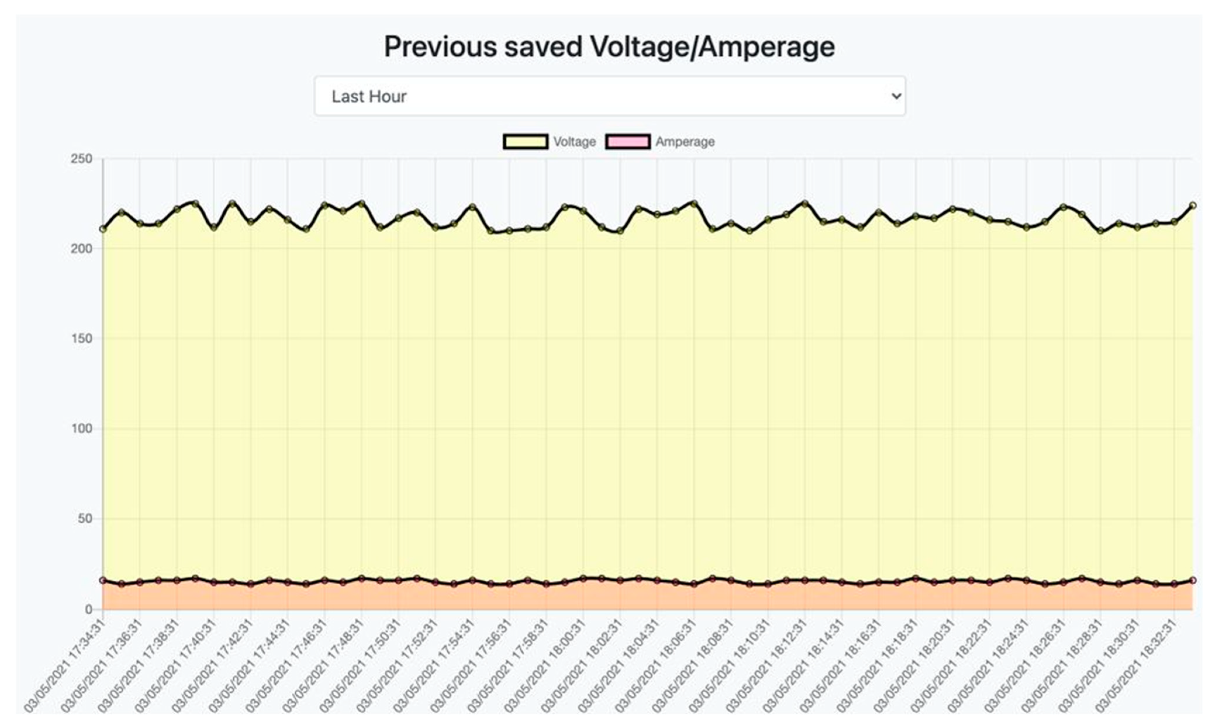
4.2.3. Experiment Results
- The display of energy characteristics in real time;
- The display of energy characteristics in the past.
5. Discussion
6. Conclusions
- The development of ontological models describing the intelligent UAV- and IoT-based monitoring systems in various situations and environmental conditions;
- The development of different separate and joint digital twin models for centers of decision making and for the implementation for optimal procedures of critical object recovery;
- The development and research of SM dependability models considering the extended taxonomy of hardware and software faults, recovery procedures and the location of the SM, as well as automated battery maintenance systems [84];
- The consideration of the cybersecurity aspects of the Internet of Drones for subsystem FCC and subsystem PCG for the assessment and assurance of SM reliability [85].
Author Contributions
Funding
Institutional Review Board Statement
Informed Consent Statement
Acknowledgments
Conflicts of Interest
Abbreviations
| Acronyms | |
| API | Application Programming Interface |
| CM | centers of control and monitoring |
| CR | control room |
| DT | digital twin |
| DTaaS | digital twin as a service |
| DTI | digital twin instance |
| EC | equipment that is monitored and controlled |
| ECS | energy consumption with sensors |
| ECR | emergency control room |
| HTTP | HyperText Transfer Protocol |
| FCC | flying control center |
| FEN | flying edge node |
| IoD | Internet of Drones |
| IoT | Internet of Things |
| JWT | JavaScript Object Notation Web Token |
| MSS | multi-state system |
| OM | objects that are monitored or/and controlled |
| PCG | private cloud crisis group |
| RBD | reliability block diagram |
| SM | monitoring system |
| UAV | unmanned aerial vehicle |
| UC | utility that is monitored and controlled |
| ZC | zones that are monitored |
| VAMF | variants of allocation of monitoring functions |
| Notation | |
| Comα_β | communications between α and β, where α = EC, UC, ZC and β = CR, ECR, PCG, FCC. |
| DMU_γ | decision-making support means in γ, where γ = CR, ECR. |
| Dtw_β/Prc_β | digital twins/data processing means in β, where β = CR, ECR, PCG, FCC. |
| coefficient by which the basic failure rate must be multiplied to obtain the failure rates of I, where I = Comα_β, DMU_γ, Dtw_β, Prc_β; α = EC, UC, ZC; β = CR, ECR, PCG, FCC; and γ = CR, ECR | |
| coefficient by which the failure rates of Comα_CR and Comψ_ECR must be multiplied to obtain their failure rates for the emergency mode, where α = EC, UC, ZC and ψ = EC, UC, ZC | |
| reliability function of i, where i = Comα_β, DMU_γ, Dtw_β, Prc_β; α = EC, UC, ZC; β = CR, ECR, PCG, FCC; and γ = CR, ECR | |
| Sen_α | sensors in α, where α = EC, UC, ZC |
| operating time | |
| basic failure rate corresponding to the failure rate of ComFCC_ZC | |
| coefficient by which the failure rate of ComZC_ω must be multiplied to obtain its failure rate for the emergency mode where ω = PCG, FCC | |
References
- De Felice, F.; Baffo, I.; Petrillo, A. Critical Infrastructures Overview: Past, Present and Future. Sustainability 2022, 14, 2233. [Google Scholar] [CrossRef]
- Sonesson, T.R.; Johansson, J.; Cedergren, A. Governance and interdependencies of critical infrastructures: Exploring mechanisms for cross-sector resilience. Saf. Sci. 2021, 142, 105383. [Google Scholar] [CrossRef]
- Bigliardi, B.; Bottani, E.; Casella, G. Enabling technologies, application areas and impact of industry 4.0: A bibliographic analysis. Proc. Manuf. 2020, 42, 322–326. [Google Scholar] [CrossRef]
- Ng, T.C.; Lau, S.Y.; Ghobakhloo, M.; Fathi, M.; Liang, M.S. The Application of Industry 4.0 Technological Constituents for Sustainable Manufacturing: A Content-Centric Review. Sustainability 2022, 14, 4327. [Google Scholar] [CrossRef]
- Al-Kaff, A.; Madridano, Á.; Campos, S.; García, F.; Martín, D.; de la Escalera, A. Emergency Support Unmanned Aerial Vehicle for Forest Fire Surveillance. Electronics 2020, 9, 260. [Google Scholar] [CrossRef]
- Chernetskyi, B.; Kharchenko, V.; Orehov, A. Wireless Sensor Network based Forest Fire Early Detection Systems: Development and Implementation. Int. J. Comput. 2022, 21, 92–99. [Google Scholar] [CrossRef]
- Berger, C.; Eichhammer, P.; Reiser, H.P.; Domaschka, J.; Hauck, F.J.; Habiger, G. A Survey on Resilience in the IoT: Taxonomy, Classification, and Discussion of Resilience Mechanisms. ACM Comput. Surv. 2022, 54, 147. [Google Scholar] [CrossRef]
- Harum, N.; Abidin, Z.; Shah, W.; Hassan, A. Implementation of smart monitoring system with fall dectector for elderly using IoT technology. Int. J. Comput. 2018, 17, 243–249. [Google Scholar] [CrossRef]
- Morozova, O.I.; Nicheporuk, A.O.; Tetskyi, A.G.; Tkachov, V.M. Methods and technologies of ensuring cybersecurity of industrial and web-oriented systems and networks. Radioelectron. Comput. Syst. 2021, 4, 145–156. [Google Scholar] [CrossRef]
- Agnusdei, G.P.; Elia, V.; Gnoni, M.G. Is Digital Twin Technology Supporting Safety Management? A Bibliometric and Systematic Review. Appl. Sci. 2021, 11, 2767. [Google Scholar] [CrossRef]
- Zheng, T.; Ardolino, M.; Bacchetti, A.; Perona, M. The applications of Industry 4.0 technologies in manufacturing context: A systematic literature review. Int. J. Prod. Res. 2021, 59, 1922–1954. [Google Scholar] [CrossRef]
- Jamwal, A.; Agrawal, R.; Sharma, M.; Giallanza, A. Industry 4.0 technologies for manufacturing sustainability: A systematic review and future research directions. Appl. Sci. 2021, 11, 5725. [Google Scholar] [CrossRef]
- di Capaci, R.B.; Scali, C. A cloud-based monitoring system for performance assessment of industrial plants. Ind. Eng. Chem. Res. 2021, 59, 2341–2352. [Google Scholar] [CrossRef]
- Stentoft, J.; Wickstrom, K.A.; Philipsen, K.; Haug, A. Drivers and barriers for Industry 4.0 readiness and practice: Empirical evidence from small and medium-sized manufacturers. Prod. Plan. Control 2021, 32, 811–828. [Google Scholar] [CrossRef]
- Meindl, B.; Ayala, N.F.; Mendonca, J.; Frank, A.G. The four smarts of Industry 4.0: Evolution of ten years of research and future perspectives. Technol. Forecast. Soc. Chang. 2021, 168, 120784. [Google Scholar] [CrossRef]
- Nara, E.O.B.; da Costa, M.B.; Baierle, I.C.; Schaefer, J.L.; Benitez, G.B.; do Santos, L.M.A.L.; Benitez, L.B. Expected impact of industry 4.0 technologies on sustainable development: A study in the context of Brazil’s plastic industry. Sust. Prod. Consum. 2021, 25, 102–122. [Google Scholar] [CrossRef]
- Tortorella, G.L.; Fogliatto, F.S.; Cauchick-Miguel, P.A.; Kurnia, S.; Jurburg, D. Integration of industry 4.0 technologies into total productive maintenance practices. Int. J. Prod. Econ. 2021, 240, 108224. [Google Scholar] [CrossRef]
- Industry 4.0 and the Digital Twin. Deloitte University Press Deloitte Development LLC. Available online: https://www2.deloitte.com/content/dam/Deloitte/kr/Documents/insights/deloitte-newsletter/2017/26_201706/kr_insights_deloitte-newsletter-26_report_02_en.pdf (accessed on 20 June 2022).
- Singh, M.; Fuenmayor, E.; Hinchy, E.P.; Qiao, Y.; Murray, N.; Devine, D. Digital Twin: Origin to Future. Appl. Syst. Innov. 2021, 4, 36. [Google Scholar] [CrossRef]
- da Silva Mendonca, R.; de Oliveira Lins, S.; de Bessa, I.V.; de Carvalho Ayres, F.A., Jr.; de Medeiros, R.L.P.; de Lucena, V.F., Jr. Digital Twin Applications: A Survey of Recent Advances and Challenges. Processes 2022, 10, 744. [Google Scholar] [CrossRef]
- van Rooij, F.; Scarf, P.; Do, P. Planning the restoration of membranes in RO desalination using a digital twin. Desalination 2021, 519, 115214. [Google Scholar] [CrossRef]
- Yitmen, I.; Alizadehsalehi, S.; Akıner, I.; Akıner, M.E. An Adapted Model of Cognitive Digital Twins for Building Lifecycle Management. Appl. Sci. 2021, 11, 4276. [Google Scholar] [CrossRef]
- Aheleroff, S.; Xu, X.; Zhong, R.Y.; Lu, Y. Digital Twin as a Service (DTaaS) in Industry 4.0: An Architecture Reference Model. Adv. Eng. Inform. 2021, 47, 101225. [Google Scholar] [CrossRef]
- Zhang, H.; Ma, L.; Sun, J.; Lin, H.; Thurer, M. Digital Twin in Services and Industrial Product Service Systems: Review and Analysis. Proc. CIRP 2019, 83, 57–60. [Google Scholar] [CrossRef]
- Padovano, A.; Longo, F.; Nicoletti, L.; Mirabelli, G. A Digital Twin based Service Oriented Application for a 4.0 Knowledge Navigation in the Smart Factory. IFAC-Pap. 2018, 51, 631–636. [Google Scholar] [CrossRef]
- Meierhofer, J.; West, S.; Rapaccini, M.; Barbieri, C. The Digital Twin as a Service Enabler: From the Service Ecosystem to the Simulation Model. In Exploring Service Science. IESS 2020. Lecture Notes in Business Information Processing; Nóvoa, H., Drăgoicea, M., Kühl, N., Eds.; Springer: Cham, Switzerland, 2020; Volume 377, pp. 347–359. [Google Scholar] [CrossRef]
- Sharma, A.; Kosasih, E.; Zhang, J.; Brintrup, A.; Calinescu, A. Digital Twins: State of the Art Theory and Practice, Challenges, and Open Research Questions. arXiv 2020, arXiv:2011.02833. [Google Scholar] [CrossRef]
- He, F.; Ong, S.K.; Nee, A.Y.C. An Integrated Mobile Augmented Reality Digital Twin Monitoring System. Computers 2021, 10, 99. [Google Scholar] [CrossRef]
- Fuller, A.; Fan, Z.; Day, C.; Barlow, C. Digital Twin: Enabling Technologies, Challenges and Open Research. IEEE Access 2020, 8, 108952–108971. [Google Scholar] [CrossRef]
- Sakhnini, J.; Karimipour, H.; Dehghantanha, A.; Parizi, M.R. AI and Security of Critical Infrastructure. In Handbook of Big Data Privacy; Choo, K.K., Dehghantanha, A., Eds.; Springer: Cham, Switzerland, 2020; pp. 7–36. [Google Scholar] [CrossRef]
- Kraidi, L.; Shah, R.; Matipa, W.; Borthwick, F. An investigation of mitigating the safety and security risks allied with oil and gas pipeline projects. J. Pipeline Sci. Eng. 2021, 1, 349–359. [Google Scholar] [CrossRef]
- Wang, X.; Wei, H.; Chen, N.; He, X.; Tian, Z. An Observational Process Ontology-Based Modeling Approach for Water Quality Monitoring. Water 2020, 12, 715. [Google Scholar] [CrossRef]
- Bragatto, P.A.; Ansaldi, S.M.; Agnello, P.; Di Condina, T.; Zanzotto, F.M.; Milazzo, M.F. Ageing management and monitoring of critical equipment at Seveso sites: An ontological approach. J. Loss Prev. Proc. Ind. 2020, 66, 104204. [Google Scholar] [CrossRef]
- Lee, S.; Sharafat, A.; Kim, I.S.; Seo, J. Development and Assessment of an Intelligent Compaction System for Compaction Quality Monitoring, Assurance, and Management. Appl. Sci. 2022, 12, 6855. [Google Scholar] [CrossRef]
- Vaccari, M.; Pannocchia, G.; Tognotti, L.; Paci, M.; Bonciani, R. A rigorous simulation model of geothermal power plants for emission control. Appl. Energy 2020, 263, 114814. [Google Scholar] [CrossRef]
- Vansovits, V.; Petlenkov, E.; Tepljakov, A.; Vassiljeva, K.; Belikov, J. Bridging the Gap in Technology Transfer for Advanced Process Control with Industrial Applications. Sensors 2022, 22, 4149. [Google Scholar] [CrossRef] [PubMed]
- Vaccari, M.; Bacci Di Capaci, R.; Brunazzi, E.; Tognotti, L.; Pierno, P.; Vagheggi, R.; Pannocchia, G. Optimally Managing Chemical Plant Operations: An Example Oriented by Industry 4.0 Paradigms. Ind. Eng. Chem. Res. 2021, 60, 7853–7867. [Google Scholar] [CrossRef]
- Vaccari, M.; di Capaci, R.B.; Brunazzi, E.; Tognotti, L.; Pierno, P.; Vagheggi, R.; Pannocchia, G. Implementation of an Industry 4.0 system to optimally manage chemical plant operation. IFAC-Pap. 2020, 53, 11545–11550. [Google Scholar] [CrossRef]
- Botín-Sanabria, D.M.; Mihaita, A.-S.; Peimbert-García, R.E.; Ramírez-Moreno, M.A.; Ramírez-Mendoza, R.A.; Lozoya-Santos, J.d.J. Digital Twin Technology Challenges and Applications: A Comprehensive Review. Remote Sens. 2022, 14, 1335. [Google Scholar] [CrossRef]
- Salem, T.; Dragomir, M. Options for and Challenges of Employing Digital Twins in Construction Management. Appl. Sci. 2022, 12, 2928. [Google Scholar] [CrossRef]
- Choi, S.; Woo, J.; Kim, J.; Lee, J.Y. Digital Twin-Based Integrated Monitoring System: Korean Application Cases. Sensors 2022, 22, 5450. [Google Scholar] [CrossRef]
- Soares, R.M.; Camara, M.M.; Feital, T.; Pinto, J.C. Digital Twin for Monitoring of Industrial Multi-Effect Evaporation. Processes 2019, 7, 537. [Google Scholar] [CrossRef]
- Kaiblinger, A.; Woschank, M. State of the Art and Future Directions of Digital Twins for Production Logistics: A Systematic Literature Review. Appl. Sci. 2022, 12, 669. [Google Scholar] [CrossRef]
- Kampczyk, A.; Dybeł, K. The Fundamental Approach of the Digital Twin Application in Railway Turnouts with Innovative Monitoring of Weather Conditions. Sensors 2021, 21, 5757. [Google Scholar] [CrossRef] [PubMed]
- Qian, C.; Liu, X.; Ripley, C.; Qian, M.; Liang, F.; Yu, W. Digital Twin—Cyber Replica of Physical Things: Architecture, Applications and Future Research Directions. Future Internet 2022, 14, 64. [Google Scholar] [CrossRef]
- Al-Ali, A.R.; Gupta, R.; Batool, T.Z.; Landolsi, T.; Aloul, F.; Al Nabulsi, A. Digital Twin Conceptual Model within the Context of Internet of Things. Future Internet 2020, 12, 163. [Google Scholar] [CrossRef]
- Stojanovic, L.; Uslander, T.; Volz, F.; Weibenbacher, C.; Muller, J.; Jacoby, M.; Bischoff, T. Methodology and Tools for Digital Twin Management—The FA3ST Approach. IoT 2021, 2, 717–740. [Google Scholar] [CrossRef]
- Immerman, D. Why IoT is the Backbone for Digital Twin. PTC. Available online: https://www.ptc.com/en/blogs/corporate/iot-digital-twin#:~:text=The%20Internet%20of%20Things%20and,virtually%20represent%20their%20physical%20counterparts (accessed on 22 June 2022).
- Lin, H.; Garg, S.; Hu, J.; Wang, X.; Piran, M.J.; Hossain, M.S. Data fusion and transfer learning empowered granular trust evaluation for Internet of Things. Inform. Fusion 2022, 78, 149–157. [Google Scholar] [CrossRef]
- Videras Rodríguez, M.; Melgar, S.G.; Cordero, A.S.; Márquez, J.M.A. A Critical Review of Unmanned Aerial Vehicles (UAVs) Use in Architecture and Urbanism: Scientometric and Bibliometric Analysis. Appl. Sci. 2021, 11, 9966. [Google Scholar] [CrossRef]
- Abdelmaboud, A. The Internet of Drones: Requirements, Taxonomy, Recent Advances, and Challenges of Research Trends. Sensors 2021, 21, 5718. [Google Scholar] [CrossRef]
- Bridgwater, T.J.F. Characterisation of a Nuclear Cave Environment Utilising an Autonomous Swarm of Heterogeneous Robots. University of the West of England and University of Bristol. Available online: https://uwe-repository.worktribe.com/output/1490801 (accessed on 22 June 2022).
- Jumaah, H.J.; Kalantar, B.; Halin, A.A.; Mansor, S.; Ueda, N.; Jumaah, S.J. Development of UAV-Based PM2.5 Monitoring System. Drones 2021, 5, 60. [Google Scholar] [CrossRef]
- Siwen, L. Development of a UAV-Based System to Monitor Air Quality over an Oil Field. Available online: https://digitalcommons.mtech.edu/grad_rsch/187/ (accessed on 22 June 2022).
- Horvath, D.; Gazda, J.; Slapak, E.; Maksymyuk, T.; Dohler, M. Evolutionary Coverage Optimization for a Self-Organizing UAV-Based Wireless Communication System. IEEE Access 2021, 9, 145066–145082. [Google Scholar] [CrossRef]
- Elmokadem, T.; Savkin, A.V. A Hybrid Approach for Autonomous Collision-Free UAV Navigation in 3D Partially Unknown Dynamic Environments. Drones 2021, 5, 57. [Google Scholar] [CrossRef]
- Stolfi, D.H.; Brust, M.R.; Danoy, G.; Bouvry, P. UAV-UGV-UMV Multi-Swarms for Cooperative Surveillance. Front. Robot. AI 2021, 8, 616950. [Google Scholar] [CrossRef] [PubMed]
- Lewis, M. Human Interaction with Multiple Remote Robots. Rev. Human Factors Ergonom. 2013, 9, 131–174. [Google Scholar] [CrossRef]
- Hussein, A.; Abbass, H. Mixed Initiative Systems for Human-Swarm Interaction: Opportunities and Challenges. IEEE Xplore 2018, 1–8. [Google Scholar] [CrossRef]
- Shubhani, A.; Neeraj, K. Path planning techniques for unmanned aerial vehicles: A review, solutions, and challenges. Comput. Commun. 2020, 149, 270–299. [Google Scholar] [CrossRef]
- Lee, W.; Lee, J.Y.; Lee, J.; Kim, K.; Yoo, S.; Park, S.; Kim, H. Ground Control System Based Routing for Reliable and Efficient Multi-Drone Control System. Appl. Sci. 2018, 8, 2027. [Google Scholar] [CrossRef]
- Shin, M.; Kim, J.; Levorato, M. Auction-based charging scheduling with deep learning framework for multi-drone networks. IEEE Trans. Veh. Technol. 2019, 68, 4235–4248. [Google Scholar] [CrossRef]
- Torabbeigi, M.; Lim, G.J.; Kim, S.J. UAV delivery schedule optimization considering the reliability of UAVs. In Proceedings of the International Conference on Unmanned Aircraft Systems (ICUAS), Dallas, TX, USA, 12–15 June 2018; pp. 1048–1053. [Google Scholar]
- Hongyan, D.; Chi, Z.; Guanghan, B.; Liwei, C. Mission reliability modeling of UAV swarm and its structure optimization based on importance measure. Rel. Eng. Syst. Saf. 2021, 215, 107879. [Google Scholar] [CrossRef]
- Mignardi, S.; Marini, R.; Verdone, R.; Buratti, C. On the Performance of a UAV-Aided Wireless Network Based on NB-IoT. Drones 2021, 5, 94. [Google Scholar] [CrossRef]
- Na, Z.; Ji, C.; Lin, B.; Zhang, N. Joint Optimization of Trajectory and Resource Allocation in Secure UAV Relaying Communications for Internet of Things. IEEE IoT J. 2022. [Google Scholar] [CrossRef]
- Islam, A.; Al Amin, A.; Shin, S.Y. FBI: A Federated Learning-Based Blockchain-Embedded Data Accumulation Scheme Using Drones for Internet of Things. IEEE Wirel. Commun. Lett. 2022, 11, 972–976. [Google Scholar] [CrossRef]
- Li, D.; Ge, S.S.; He, W.; Ma, G.; Xie, L. Multilayer formation control of multi-agent systems. Automatica 2019, 109, 108558. [Google Scholar] [CrossRef]
- Herrera, M.; Parlikad, A.K.; Izquierdo, J.; Perez Hernandez, M. Multi-Agent Systems and Complex Networks: Review and Applications in Systems Engineering. Processes 2020, 8, 312. [Google Scholar] [CrossRef]
- Shafiq, M.; Ali, Z.A.; Alkhammash, E.H. A Cluster-Based Hierarchical-Approach for the Path Planning of Swarm. Appl. Sci. 2021, 11, 6864. [Google Scholar] [CrossRef]
- Fesenko, H.; Kharchenko, V.; Sachenko, A.; Hiromoto, R.; Kochan, V. Chapter 9—An internet of drone-based multi-version post-severe accident monitoring system: Structures and reliability. In Dependable IoT for Human and Industry: Modeling, Architecting, Implementation; Kharchenko, V., Kor, A.L., Rucinski, A., Eds.; River Publishers: Gistrup, Denmark, 2018; pp. 197–217. [Google Scholar]
- Abarnikov, Y.; Kharchenko, V.; Morozova, O. Equipment monitoring system with use of Digital Twins and Internet of Things: Algorithms, architecting and experiments. In Proceedings of the 11th IEEE International Conference on Intelligent Data Acquisition and Advanced Computing Systems: Technology and Applications (IDAACS), Krakow, Poland, 22–25 September 2021; Volume 1, pp. 75–80. [Google Scholar]
- Kharchenko, V.; Sachenko, A.; Kochan, V.; Fesenko, H. Reliability and survivability models of integrated drone-based systems for post emergency monitoring of NPPs. In Proceedings of the International Conference on Information and Digital Technologies (IDT), Rzeszow, Poland, 5–7 July 2016; pp. 127–132. [Google Scholar] [CrossRef]
- Kliushnikov, I.; Fesenko, H.; Kharchenko, V. Scheduling UAV Fleets for The Persistent Operation of UAV-Enabled Wireless Networks During NPP Monitoring. Radioelectron. Comput. Syst. 2020, 1, 29–36. [Google Scholar] [CrossRef]
- Lisnianski, A.; Frenkel, I.; Ding, Y. Multi-State System Reliability Analysis and Optimization for Engineers and Industrial Managers; Springer-Verlag: London, UK, 2010; pp. 1–28. [Google Scholar] [CrossRef]
- Sachenko, A.; Kochan, V.; Kharchenko, V.; Roth, H.; Yatskiv, V.; Chernyshov, M.; Bykovyy, P.; Roshchupkin, O.; Koval, V.; Fesenko, H. Mobile Post-Emergency Monitoring System for Nuclear Power Plants. In Proceedings of the ICT in Education, Research and Industrial Applications (ICTERI), Kyiv, Ukraine, 21–24 June 2016; pp. 384–398. [Google Scholar]
- Yastrebenetsky, M.; Kharchenko, V. Cyber Security and Safety of Nuclear Power Plant Instrumentation and Control; IGI-Global: Hershey, PA, USA, 2020; p. 501. [Google Scholar] [CrossRef]
- Ushakov, I. Probabilistic Reliability Models; JohnWiley & Sons: Hoboken, NJ, USA, 2012; pp. 20–22. Available online: https://www.wiley.com/en-us/Probabilistic+Reliability+Models-p-9781118370766 (accessed on 22 June 2022).
- A Solution That Turns Ordinary Factories into SMART in 15 Minutes. Available online: https://www.koeebox.com/ (accessed on 22 June 2022).
- Siriwardena, P. Message-Level Security with JSON Web Signature. In Advanced API Security; Apress: Berkeley, CA, USA, 2019; pp. 157–184. Available online: https://www.oreilly.com/library/view/advanced-api-security/9781484220504/A323855_2_En_7_Chapter.html (accessed on 22 June 2022).
- Fukuda, S.; Kurihara, S.; Hamanaka, S.; Oguchi, M.; Yamaguchi, S. Accelerated test for applications with client application and server software. In Proceedings of the 11th International Conference on Ubiquitous Information Management and Communication (IMCOM), Beppu, Japan, 5–7 January 2017; pp. 1–6. [Google Scholar]
- Kesavan, S.; Saravana Kumar, E.; Kumar, A.; Vengatesan, K. An investigation on adaptive HTTP media streaming Quality-of-Experience (QoE) and agility using cloud media services. Int. J. Comput. Appl. 2021, 43, 431–444. [Google Scholar] [CrossRef]
- Murley, P.; Ma, Z.; Mason, J.; Bailey, M.; Kharraz, A. WebSocket Adoption and the Landscape of the Real-Time Web. In Proceedings of the Web Conference, Ljubljana, Slovenia, 19–23 April 2021; pp. 1192–1203. [Google Scholar] [CrossRef]
- Kliushnikov, I.; Fesenko, H.; Kharchenko, V.; Illiashenko, O.; Morozova, O. UAV fleet based accident monitoring systems with automatic battery replacement systems: Algorithms for justifying composition and use planning. Int. J. Saf. Secur. Eng. 2021, 11, 319–328. [Google Scholar] [CrossRef]
- Pevnev, V.; Torianyk, V.; Kharchenko, V. Cyber Security of Wireless Smart Systems: Channels of Intrusions and Radio Frequency Vulnerabilities. Radioelectron. Comput. Syst. 2020, 4, 79–92. [Google Scholar] [CrossRef]


| Mode | Centers of Control and Monitoring | |||
|---|---|---|---|---|
| CR | ECR | FCC | PCG | |
| Normal | Monitoring EC, UC, ZC | Monitoring UC, ZC | Waiting (self-maintenance) | Waiting (self-maintenance) |
| Emergency | Monitoring EC, UC, ZC | Monitoring UC, ZC | Monitoring ZC | Monitoring ZC |
| Mode | Level | Centers of Control and Monitoring | |||
|---|---|---|---|---|---|
| CR | ECR | FCC | PCG | ||
| Normal | EC | Full | None | None | None |
| UC | Full | Full | None | None | |
| ZC | Full | Full | None | None | |
| Emergency | EC | Full | None | None | None |
| UC | Full | Full | None | None | |
| ZC | Full | Full | Full/Partial | Full/Partial | |
| Mode | Source of Information | Centers and Subsystems | Type of Structure |
|---|---|---|---|
| Normal | EC | CR | T1 |
| Normal | EC | CR | T2 |
| Normal | UC | CR, ECR | T1 |
| Normal | UC | CR, ECR | T2 |
| Normal | ZC | CR, ECR | T1 |
| Normal | ZC | CR, ECR | T2 |
| Emergency | EC | CR | T1 |
| Emergency | EC | CR | T2 |
| Emergency | UC | CR, ECR | T1 |
| Emergency | UC | CR, ECR | T2 |
| Emergency | ZC | CR, ECR, PCG*, FCC* | T1 |
| Emergency | ZC | CR, ECR, PCG*, FCC* | T2 |
| Emergency | ZC | CR, ECR, PCG, FCC* | T1 |
| Emergency | ZC | CR, ECR, PCG, FCC* | T2 |
| Emergency | ZC | CR, ECR, FCC, PCG* | T1 |
| Emergency | ZC | CR, ECR, FCC, PCG* | T2 |
| Emergency | ZC | CR, ECR, PCG, FCC | T1 |
| Emergency | ZC | CR, ECR, PCG, FCC | T2 |
| Name | Possibility of Using the Device KOEEBOX | How It Can Be Used | Working Principle |
|---|---|---|---|
| CR/ECR | + | Control and monitoring of the equipment of the center | Collects and analyzes statistics on power supply of equipment |
| PCG | + | Server monitoring | Monitors server power status |
| FCC | + | Control and monitoring station | Monitors control panels status |
Publisher’s Note: MDPI stays neutral with regard to jurisdictional claims in published maps and institutional affiliations. |
© 2022 by the authors. Licensee MDPI, Basel, Switzerland. This article is an open access article distributed under the terms and conditions of the Creative Commons Attribution (CC BY) license (https://creativecommons.org/licenses/by/4.0/).
Share and Cite
Sun, Y.; Fesenko, H.; Kharchenko, V.; Zhong, L.; Kliushnikov, I.; Illiashenko, O.; Morozova, O.; Sachenko, A. UAV and IoT-Based Systems for the Monitoring of Industrial Facilities Using Digital Twins: Methodology, Reliability Models, and Application. Sensors 2022, 22, 6444. https://doi.org/10.3390/s22176444
Sun Y, Fesenko H, Kharchenko V, Zhong L, Kliushnikov I, Illiashenko O, Morozova O, Sachenko A. UAV and IoT-Based Systems for the Monitoring of Industrial Facilities Using Digital Twins: Methodology, Reliability Models, and Application. Sensors. 2022; 22(17):6444. https://doi.org/10.3390/s22176444
Chicago/Turabian StyleSun, Yun, Herman Fesenko, Vyacheslav Kharchenko, Luo Zhong, Ihor Kliushnikov, Oleg Illiashenko, Olga Morozova, and Anatoliy Sachenko. 2022. "UAV and IoT-Based Systems for the Monitoring of Industrial Facilities Using Digital Twins: Methodology, Reliability Models, and Application" Sensors 22, no. 17: 6444. https://doi.org/10.3390/s22176444
APA StyleSun, Y., Fesenko, H., Kharchenko, V., Zhong, L., Kliushnikov, I., Illiashenko, O., Morozova, O., & Sachenko, A. (2022). UAV and IoT-Based Systems for the Monitoring of Industrial Facilities Using Digital Twins: Methodology, Reliability Models, and Application. Sensors, 22(17), 6444. https://doi.org/10.3390/s22176444