
Improved LDTW Algorithm Based on the Alternating Matrix and the Evolutionary Chain Tree


Abstract
:1. Introduction
- (1)
- A two-channel matrix with an alternating scheme is proposed for similarity calculation.
- (2)
- A chain tree with an evolutionary scheme is proposed to find the optimal warping path with the similarity calculation process simultaneously.
2. Preliminary
2.1. DTW
- (1)
- ,;
- (2)
- if and , then , .
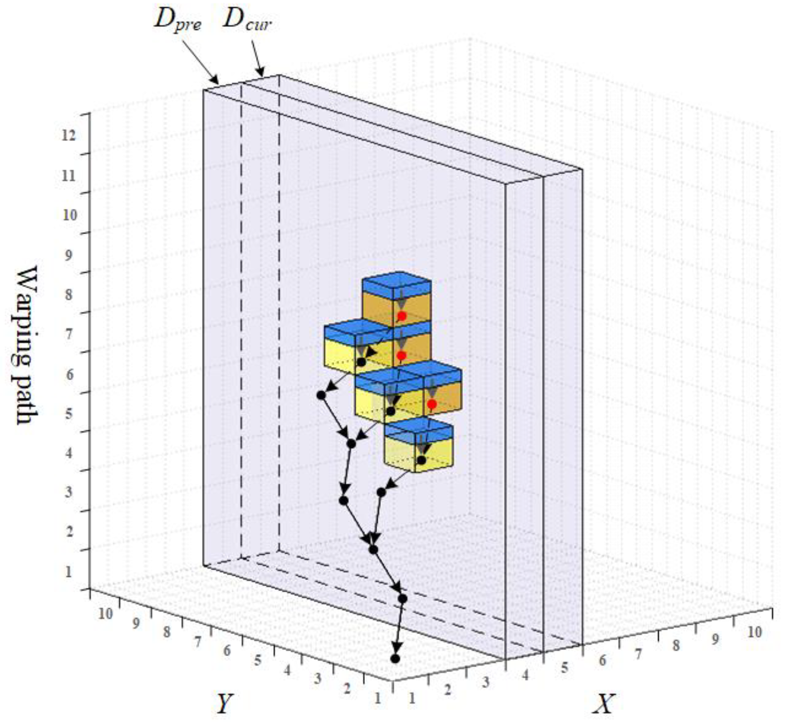
2.2. LDTW
3. The Proposed Method
3.1. The Alternating Matrix Based Similarity Calculation
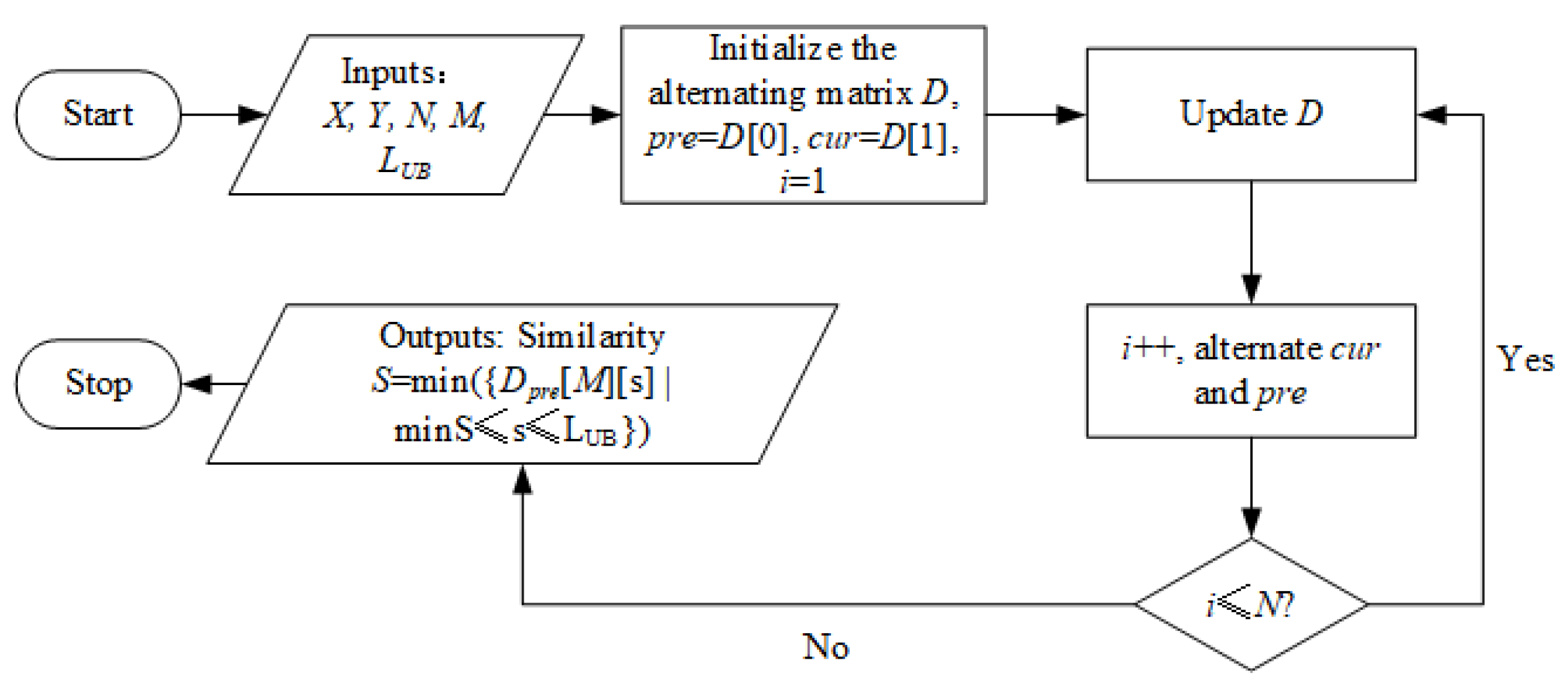
| Algorithm 1: AM Update | |
| Input: X, Y, N, M, D, i, cur, pre, LUB | |
| Ouput: updated D | |
| 1 | for j from 1 to M do |
| 2 | minS←MinStep(i, j), maxS←MaxStep(i, j, N, M, LUB) |
| 3 | if minS < maxS do |
| 4 | for s from minS to maxS do |
| 5 | |
| 6 | end for |
| 7 | end if |
| 8 | end for |
| 9 | |
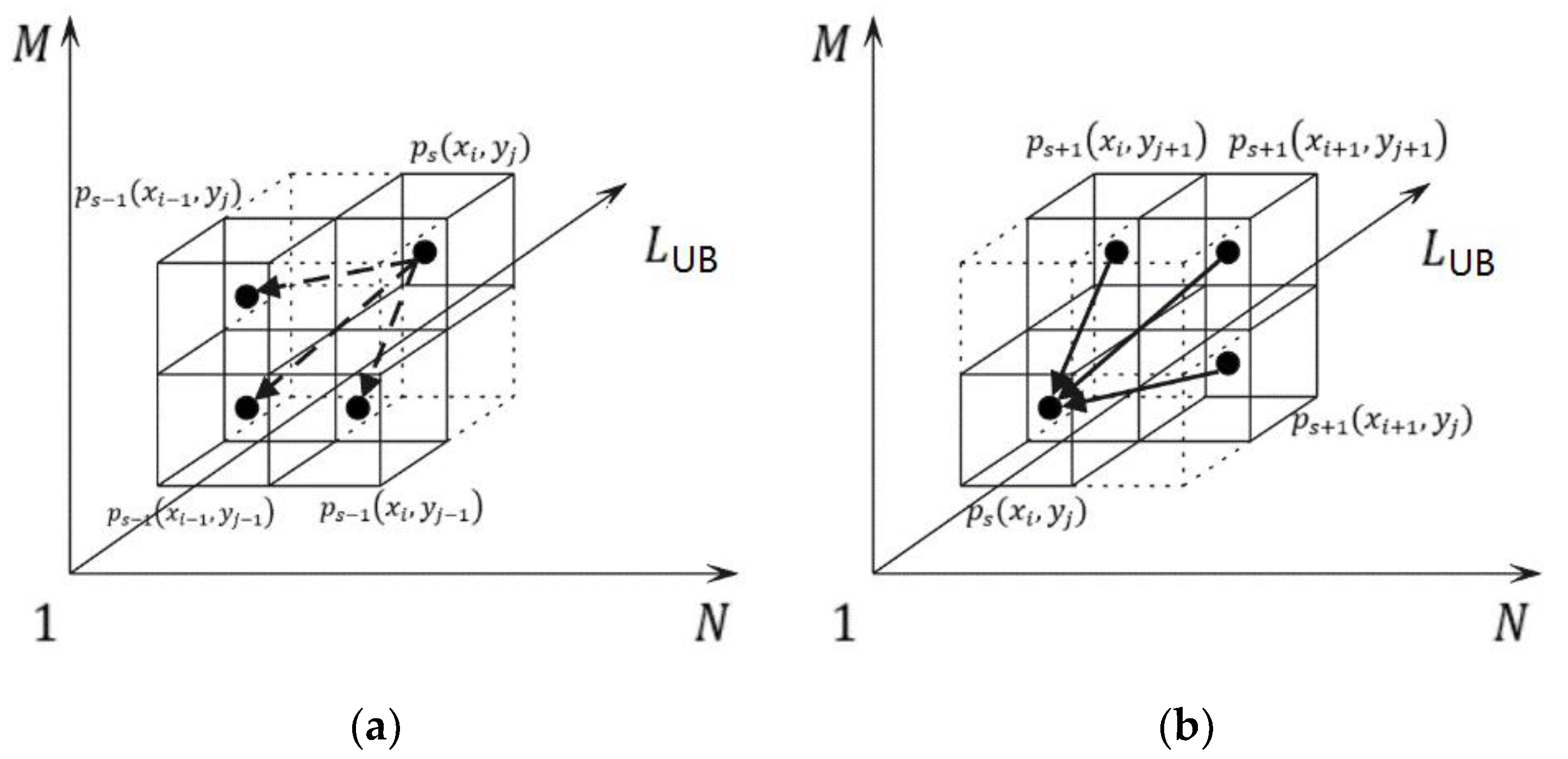
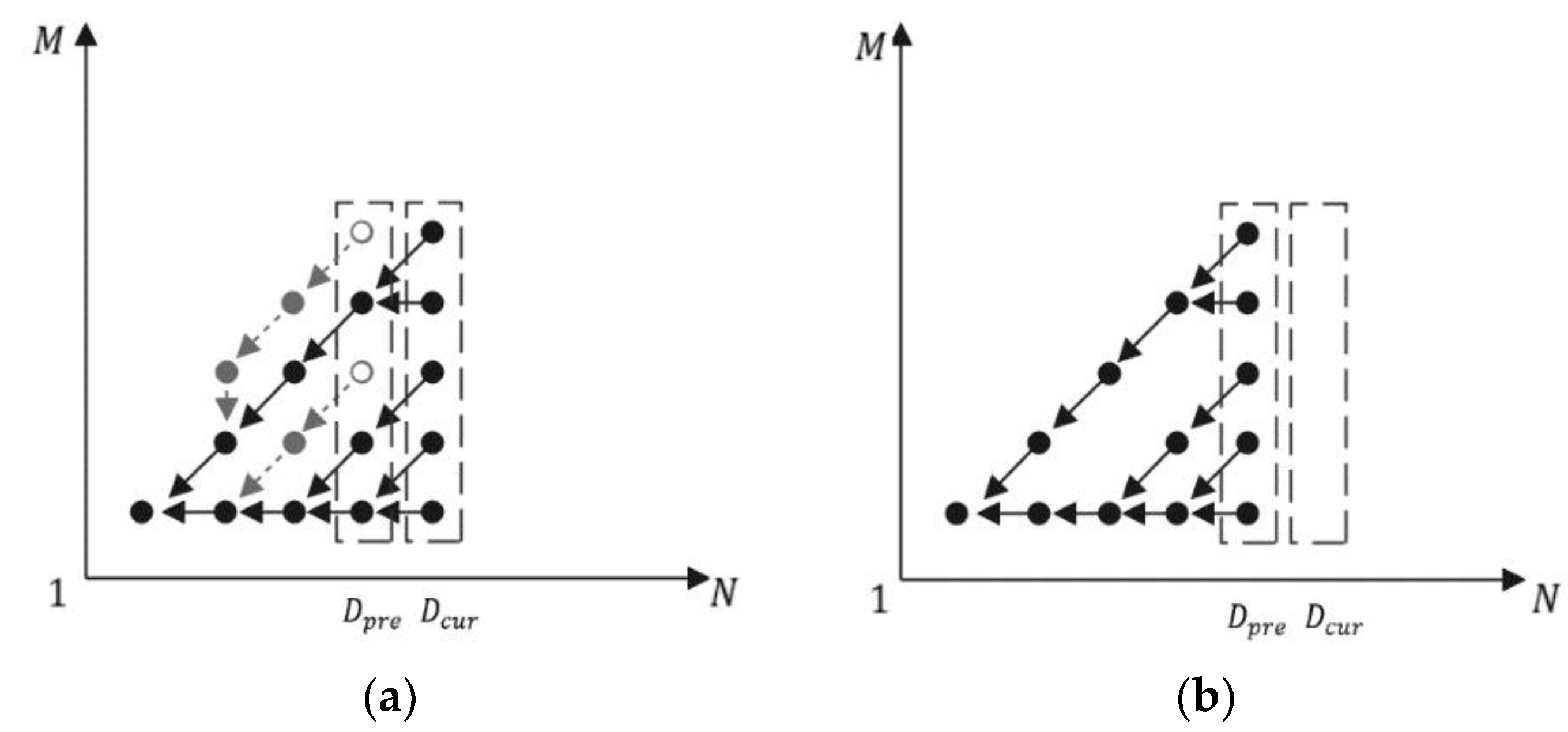
3.2. The Evolutionary Chain Tree Based Optimal Warping Path Determination
3.2.1. Growing
| Algorithm 2: ECT Growing | |
| Input: N, M, D, i, cur, pre, LUB | |
| Ouput: updated D | |
| 1 | for j from 1 to M do |
| 2 | minS←MinStep(i, j), maxS←MaxStep(i, j, N, M, LUB) |
| 3 | if minS < maxS do |
| 4 | for s from minS to maxS do |
| 5 | |
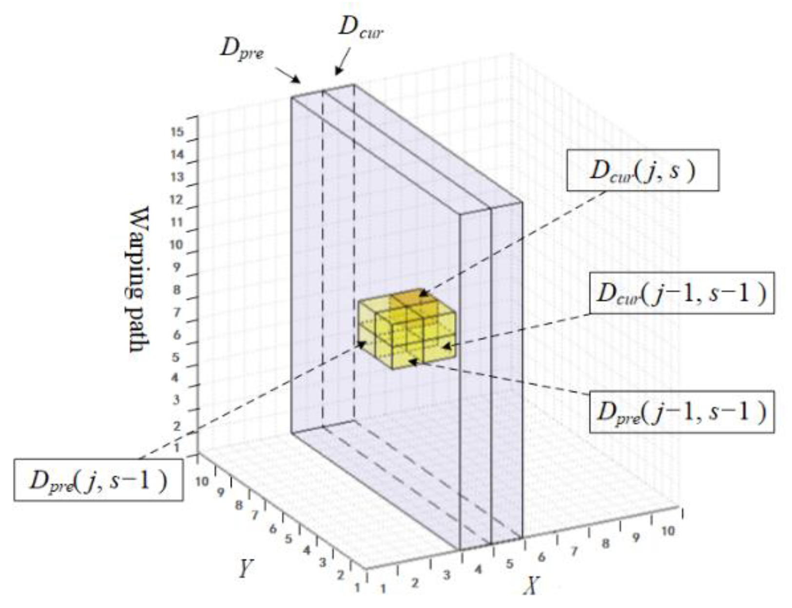
| 6 | q←min{Dpre [j][s−1], Dpre [j-1][s−1], Dcur [j-1][s−1]} |
| 7 | |
| 8 | |
| 9 | end for |
| 10 | end if |
| 11 | end for |
3.2.2. Pruning
| Algorithm 3: ECT Pruning | |
| Input: N, M, D, i, cur, pre, LUB | |
| Ouput: updated D | |
| 1 | for j from 1 to M do |
| 2 | minS←MinStep(i−1, j), maxS←MaxStep(i−1, j, N, M, LUB) |
| 3 | if minS < maxS do |
| 4 | for s from minS to maxS do |
| 5 | |
| 6 | while lower(p.data) equal to 0b00 do |
| 7 | q←p, p←p.prior, p.data--, delete q |
| 8 | end while |
| 9 | end for |
| 10 | end if |
| 11 | end for |
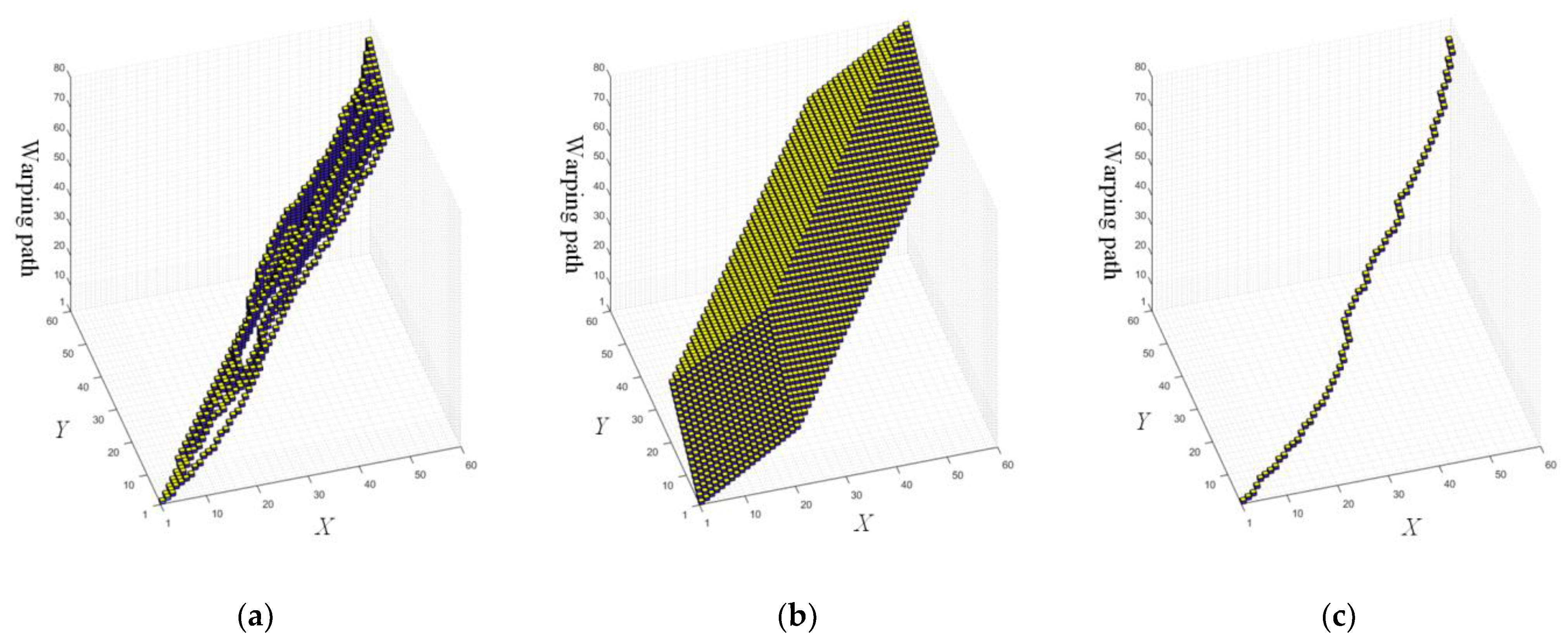
4. Experiments and Results
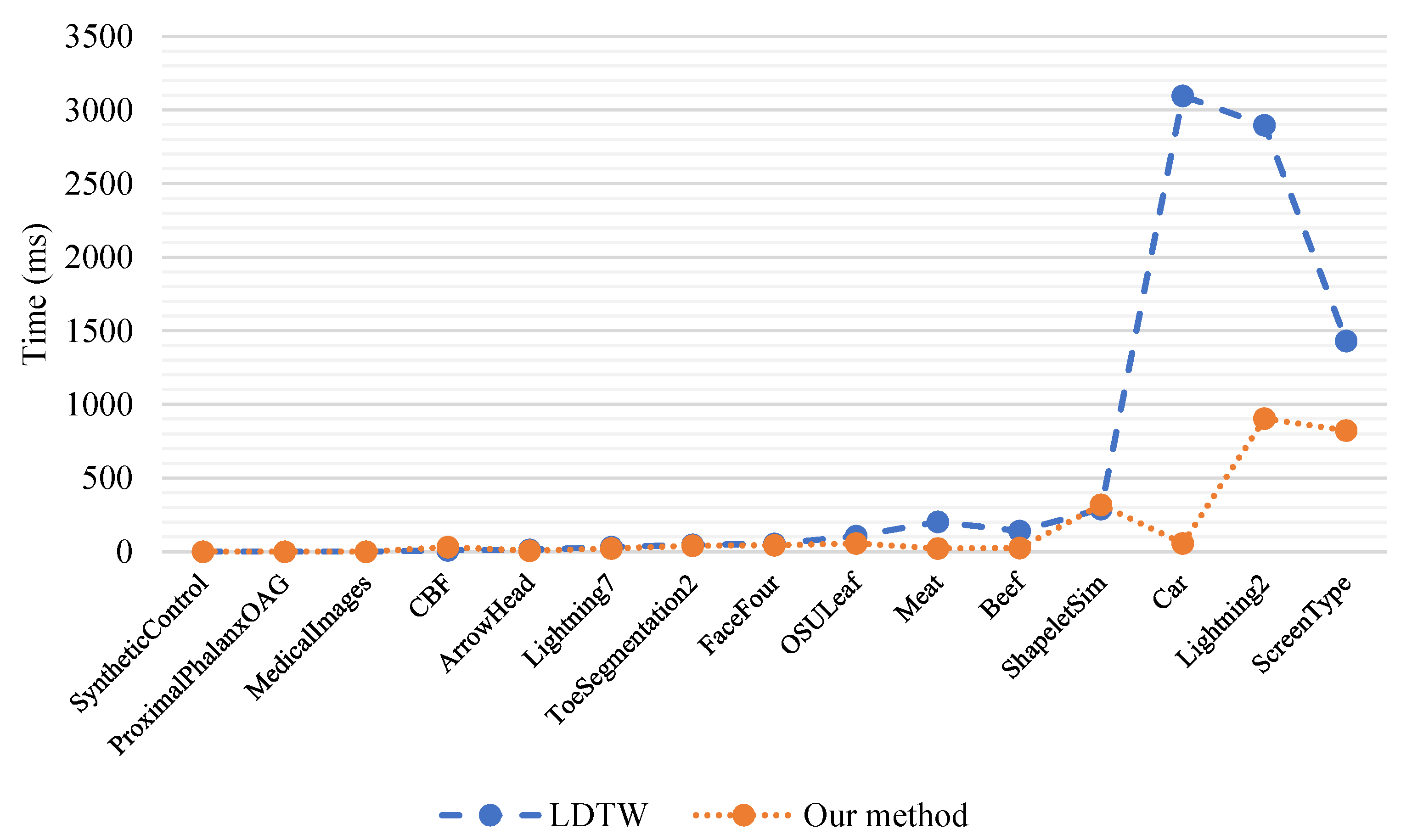
4.1. Comparisons
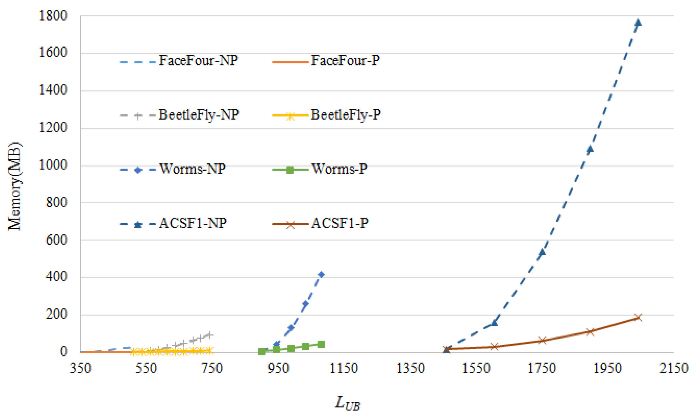
4.2. Ablation Experiment
5. Discussion
6. Conclusions
Author Contributions
Funding
Institutional Review Board Statement
Informed Consent Statement
Data Availability Statement
Conflicts of Interest
References
- Lichtenauer, J.F.; Hendriks, E.A.; Reinders, M.J. Sign language recognition by combining statistical DTW and independent classification. IEEE Trans. Pattern Anal. 2008, 30, 2040–2046. [Google Scholar] [CrossRef]
- Zhang, Z.; Tang, P.; Hu, C.; Liu, Z.; Zhang, W.; Tang, L. Seeded Classification of Satellite Image Time Series with Lower-Bounded Dynamic Time Warping. Remote Sens. 2022, 14, 2778. [Google Scholar] [CrossRef]
- Amerineni, R.; Gupta, L.; Steadman, N.; Annauth, K.; Burr, C.; Wilson, S.; Barnaghi, P.; Vaidyanathan, R. Fusion Models for Generalized Classification of Multi-Axial Human Movement: Validation in Sport Performance. Sensors 2021, 21, 8409. [Google Scholar] [CrossRef] [PubMed]
- Li, J.; Zhang, H.; Dong, Y.; Zuo, T.; Xu, D. An Improved Self-Training Method for Positive Unlabeled Time Series Classification Using DTW Barycenter Averaging. Sensors 2021, 21, 7414. [Google Scholar] [CrossRef]
- Lei, T.C.; Wan, S.; Wu, Y.C.; Wang, H.-P.; Hsieh, C.-W. Multi-Temporal Data Fusion in MS and SAR Images Using the Dynamic Time Warping Method for Paddy Rice Classification. Agriculture 2022, 12, 77. [Google Scholar] [CrossRef]
- Kumar, D.; Wu, H.; Rajasegarar, S.; Leckie, C.; Krishnaswamy, S.; Palaniswami, M. Fast and scalable big data trajectory clustering for understanding urban mobility. IEEE Trans. Intell. Transp. 2018, 19, 3709–3722. [Google Scholar] [CrossRef]
- Petitjean, F.; Ketterlin, A.; Gançarski, P. A global averaging method for dynamic time warping, with applications to clustering. Pattern Recogn. 2011, 44, 678–693. [Google Scholar] [CrossRef]
- Jiang, Y.; Qi, Y.; Wang, W.K.; Bent, B.; Avram, R.; Olgin, J.; Dunn, J. EventDTW: An Improved Dynamic Time Warping Algorithm for Aligning Biomedical Signals of Nonuniform Sampling Frequencies. Sensors 2020, 20, 2700. [Google Scholar] [CrossRef]
- He, Y.; Zhang, X.; Wang, R.; Cheng, M.; Gao, Z.; Zhang, Z.; Yu, W. Faulty Section Location Method Based on Dynamic Time Warping Distance in a Resonant Grounding System. Energies 2022, 15, 4923. [Google Scholar] [CrossRef]
- Debella, T.T.; Shawel, B.S.; Devanne, M.; Weber, J.; Woldegebreal, D.H.; Pollin, S.; Forestier, G. Deep Representation Learning for Cluster-Level Time Series Forecasting. Eng. Proc. 2022, 18, 22. [Google Scholar]
- Cui, J.-W.; Li, Z.-G.; Du, H.; Yan, B.-Y.; Lu, P.-D. Recognition of Upper Limb Action Intention Based on IMU. Sensors 2022, 22, 1954. [Google Scholar] [CrossRef]
- Zhao, S.; Cai, H.; Li, W.; Liu, Y.; Liu, C. Hand Gesture Recognition on a Resource-Limited Interactive Wristband. Sensors 2021, 21, 5713. [Google Scholar] [CrossRef]
- Li, T.; Shi, C.; Li, P.; Chen, P. A Novel Gesture Recognition System Based on CSI Extracted from a Smartphone with Nexmon Firmware. Sensors 2021, 21, 222. [Google Scholar] [CrossRef]
- Li, H.; Khoo, S.; Yap, H.J. Implementation of Sequence-Based Classification Methods for Motion Assessment and Recognition in a Traditional Chinese Sport (Baduanjin). Int. J. Environ. Res. Public Health 2022, 19, 1744. [Google Scholar] [CrossRef]
- Berndt, D.J.; Clifford, J. Using dynamic time warping to find patterns in time series. In Proceedings of the Knowledge Discovery and Data Mining Workshop, Seattle, WA, USA, 31 July 1994. [Google Scholar]
- Phan, T.T.H.; Caillault, E.P.; Lefebvre, A.; Bigand, A. Dynamic time warping-based imputation for univariate time series data. Pattern Recogn. Lett. 2020, 139, 139–147. [Google Scholar] [CrossRef] [Green Version]
- Guo, F.; Zou, F.; Luo, S.; Liao, L.; Wu, J.; Yu, X.; Zhang, C. The Fast Detection of Abnormal ETC Data Based on an Improved DTW Algorithm. Electronics 2022, 11, 1981. [Google Scholar] [CrossRef]
- Chang, C.; Shaw, T.; Goutam, A.; Lau, C.; Shan, M.; Tsai, T.J. Parameter-Free Ordered Partial Match Alignment with Hidden State Time Warping. Appl. Sci. 2022, 12, 3783. [Google Scholar] [CrossRef]
- Gong, L.; Chen, B.; Xu, W.; Liu, C.; Li, X.; Zhao, Z.; Zhao, L. Motion Similarity Evaluation between Human and a Tri-Co Robot during Real-Time Imitation with a Trajectory Dynamic Time Warping Model. Sensors 2022, 22, 1968. [Google Scholar] [CrossRef]
- Combes, F.; Fraiman, R.; Ghattas, B. Time Series Sampling. Eng. Proc. 2022, 18, 32. [Google Scholar]
- Zhang, Z.; Tavenard, R.; Bailly, A.; Tang, X.; Tang, P.; Corpetti, T. Dynamic time warping under limited warping path length. Inform. Sciences 2017, 393, 91–107. [Google Scholar]
- Sakoe, H.; Chiba, S. Dynamic programming algorithm optimization for spoken word recognition. IEEE Trans. Acoust. Speech Signal Process. 1978, 26, 43–49. [Google Scholar] [CrossRef] [Green Version]
- Anantasech, P.; Ratanamahatana, C.A. Enhanced weighted dynamic time warping for time series classification. In Proceedings of the Third International Congress on Information and Communication Technology, London, UK, 27–28 February 2018. [Google Scholar]
- Jeong, Y.S.; Jeong, M.K.; Omitaomu, O.A. Weighted dynamic time warping for time series classification. Pattern Recogn. 2011, 44, 2231–2240. [Google Scholar] [CrossRef]
- Ratanamahatana, C.A.; Keogh, E. Making time-series classification more accurate using learned constraints. In Proceedings of the 2004 SIAM International Conference on Data Mining, Lake Buena Vista, FL, USA, 22–24 April 2004. [Google Scholar]
- Dau, H.A.; Bagnall, A.; Kamgar, K.; Yeh, C.C.M.; Zhu, Y.; Gharghabi, S.; Ratanamahatana, C.A.; Keogh, E. The UCR time series archive. IEEE/CAA J. Automatic. 2019, 6, 1293–1305. [Google Scholar] [CrossRef]
- Cao, Y.; Ma, S.; Cao, Y.; Pan, G.; Huang, Q.; Cao, Y. Similarity Evaluation Rule and Motion Posture Optimization for a Manta Ray Robot. J. Mar. Sci. Eng. 2022, 10, 908. [Google Scholar] [CrossRef]


| 0b01 | 0b10 | 0b11 |
| Data Name | Length | LDTW(MB) | Our Method | ||
|---|---|---|---|---|---|
| Ph1 (MB) | Ph2 (MB) | Total (MB) | |||
| SyntheticControl | 60 | 1.02 | 0.03 | 0.01 | 0.04 |
| ProximalPhalanxOAG | 80 | 1.95 | 0.05 | 0.00 | 0.05 |
| MedicalImages | 99 | 3.89 | 0.08 | 0.01 | 0.09 |
| CBF | 128 | 12.75 | 0.20 | 0.25 | 0.45 |
| ArrowHead | 251 | 60.32 | 0.48 | 0.00 | 0.48 |
| Lightning7 | 319 | 132.76 | 0.83 | 0.13 | 0.96 |
| ToeSegmentation2 | 343 | 169.64 | 0.99 | 0.31 | 1.30 |
| FaceFour | 350 | 180.85 | 1.03 | 0.25 | 1.29 |
| OSULeaf | 427 | 321.33 | 1.51 | 0.47 | 1.98 |
| Meat | 448 | 343.00 | 1.53 | 0.00 | 1.53 |
| Beef | 470 | 400.27 | 1.70 | 0.02 | 1.72 |
| ShapeletSim | 500 | 567.44 | 2.27 | 0.91 | 3.18 |
| Car | 577 | 755.66 | 2.62 | 0.12 | 2.74 |
| Lightning2 | 637 | 1211.99 | 3.81 | 4.40 | 8.21 |
| ScreenType | 720 | 1657.18 | 4.60 | 15.39 | 19.99 |
| Data | FaceFour | BeetleFly | Worms | ACSF1 |
| Scale | 350 × 350 | 512 × 512 | 900 × 900 | 1460 × 1460 |
Publisher’s Note: MDPI stays neutral with regard to jurisdictional claims in published maps and institutional affiliations. |
© 2022 by the authors. Licensee MDPI, Basel, Switzerland. This article is an open access article distributed under the terms and conditions of the Creative Commons Attribution (CC BY) license (https://creativecommons.org/licenses/by/4.0/).
Share and Cite
Zou, Z.; Nie, M.-X.; Liu, X.-S.; Liu, S.-J. Improved LDTW Algorithm Based on the Alternating Matrix and the Evolutionary Chain Tree. Sensors 2022, 22, 5305. https://doi.org/10.3390/s22145305
Zou Z, Nie M-X, Liu X-S, Liu S-J. Improved LDTW Algorithm Based on the Alternating Matrix and the Evolutionary Chain Tree. Sensors. 2022; 22(14):5305. https://doi.org/10.3390/s22145305
Chicago/Turabian StyleZou, Zheng, Ming-Xing Nie, Xing-Sheng Liu, and Shi-Jian Liu. 2022. "Improved LDTW Algorithm Based on the Alternating Matrix and the Evolutionary Chain Tree" Sensors 22, no. 14: 5305. https://doi.org/10.3390/s22145305
APA StyleZou, Z., Nie, M.-X., Liu, X.-S., & Liu, S.-J. (2022). Improved LDTW Algorithm Based on the Alternating Matrix and the Evolutionary Chain Tree. Sensors, 22(14), 5305. https://doi.org/10.3390/s22145305