Quantized Residual Preference Based Linkage Clustering for Model Selection and Inlier Segmentation in Geometric Multi-Model Fitting

Abstract
1. Introduction
2. Materials and Methods
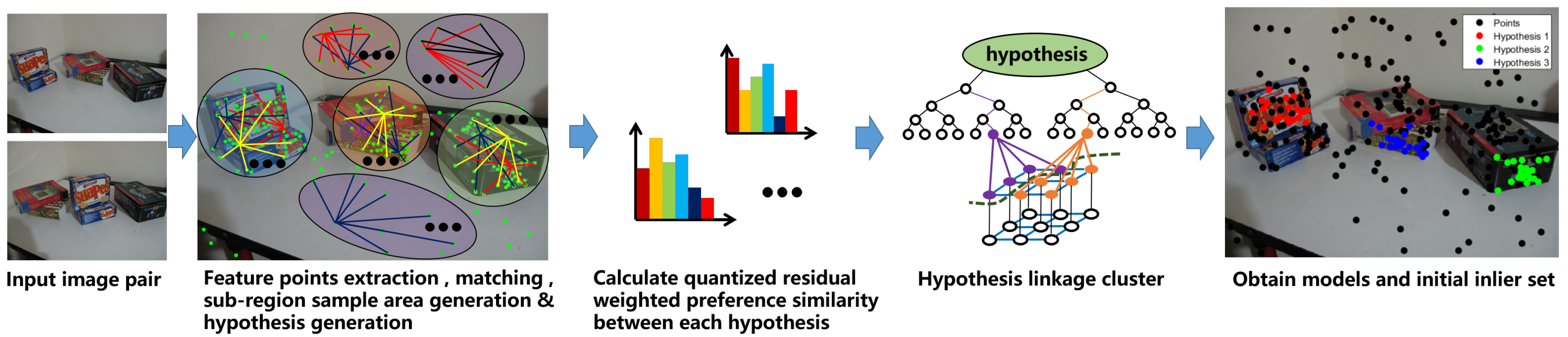
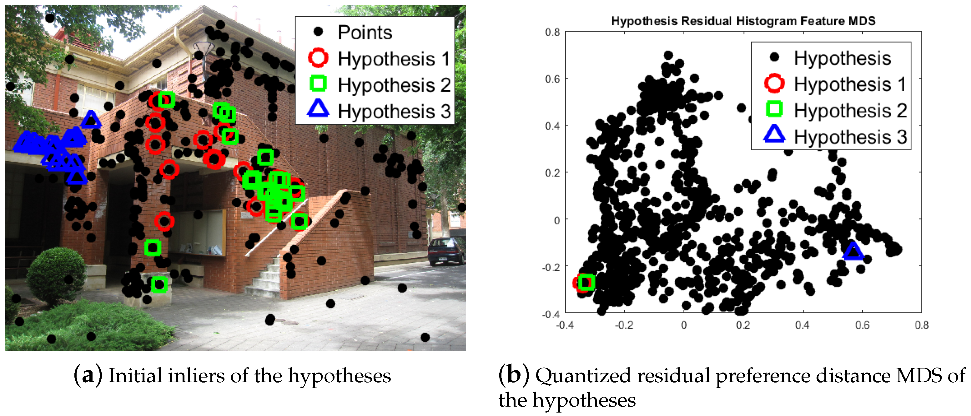
2.1. Model Selection
| Algorithm 1 | |
| 1: | Calculate hypothesis cost for each hypothesis by Equation (1); |
| 2: | Calculate quantized residual preference for hypotheses by Equations (2) and (3); |
| 3: | Calculate the weighted preference similarity by Equation (4) between every two hypotheses, and obtained similarity matrix; |
| 4: | Define each hypothesis as a cluster; |
| 5: | Merge the two cluster with maximum weighted preference similarity into one cluster; |
| 6: | Update the merged cluster with the quantized residual preference of smaller hypothesis, and replace the cluster similarity, while set the similarity of the other cluster to 0; |
| 7: | Repeat from step 5, until the maximum weighted preference similarity is less ; |
| 8: | remove the clusters whose size is less than hypothesis number. |
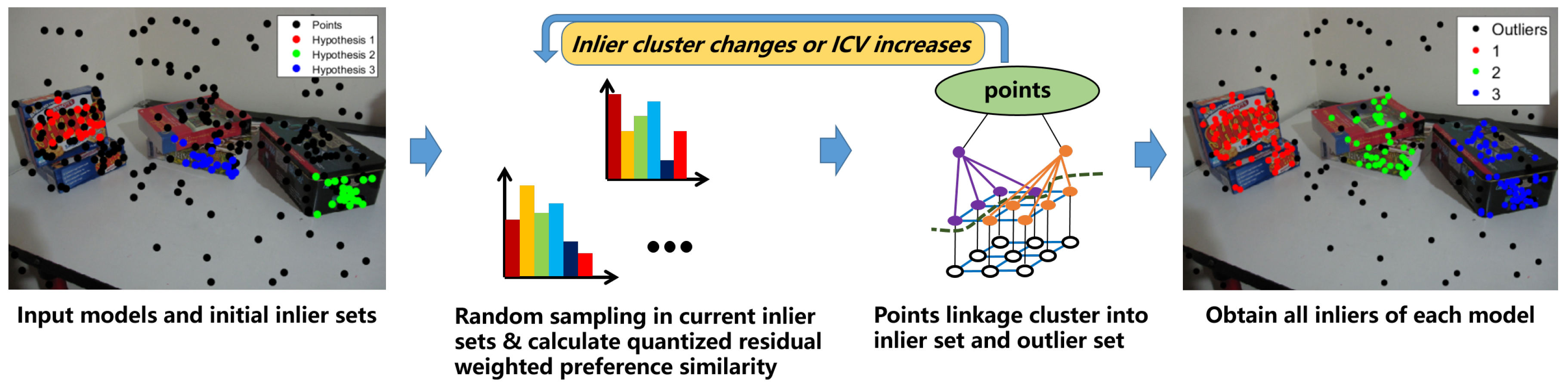
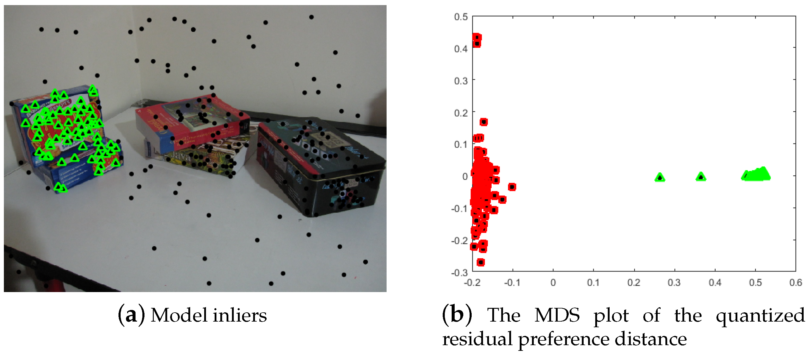
2.2. Inlier Segmentation
| Algorithm 2 |
|
3. Experiment
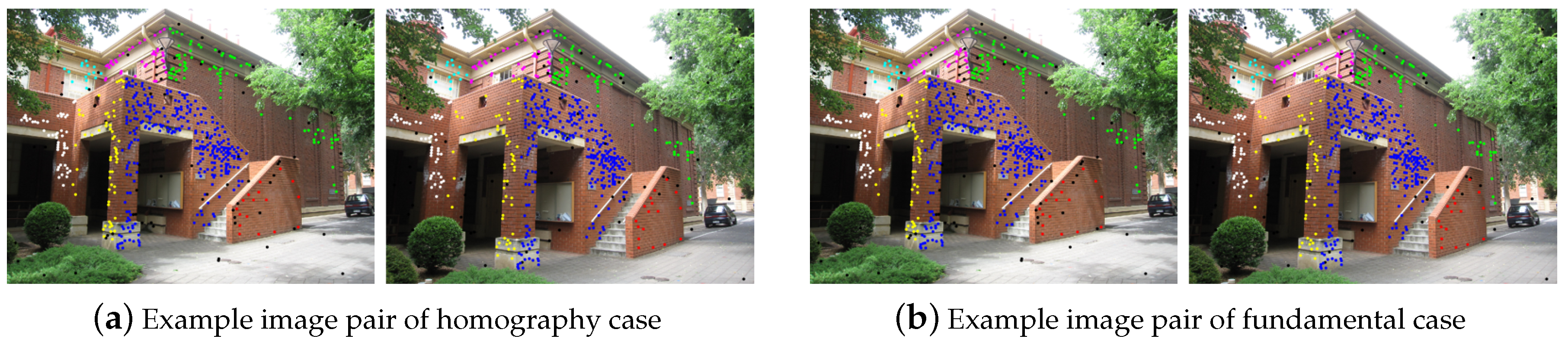
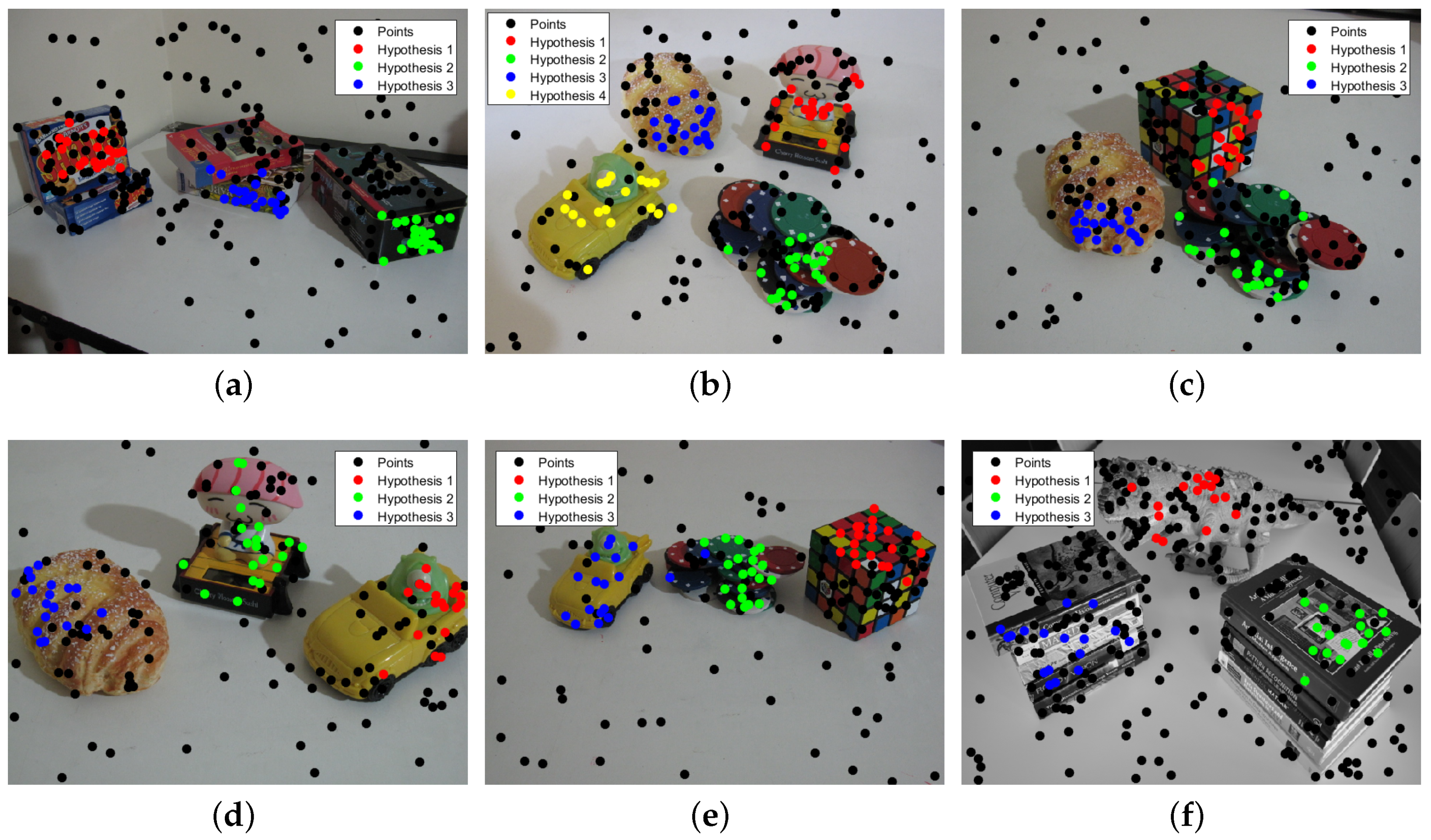
3.1. Multi-Homography Matrix Estimation
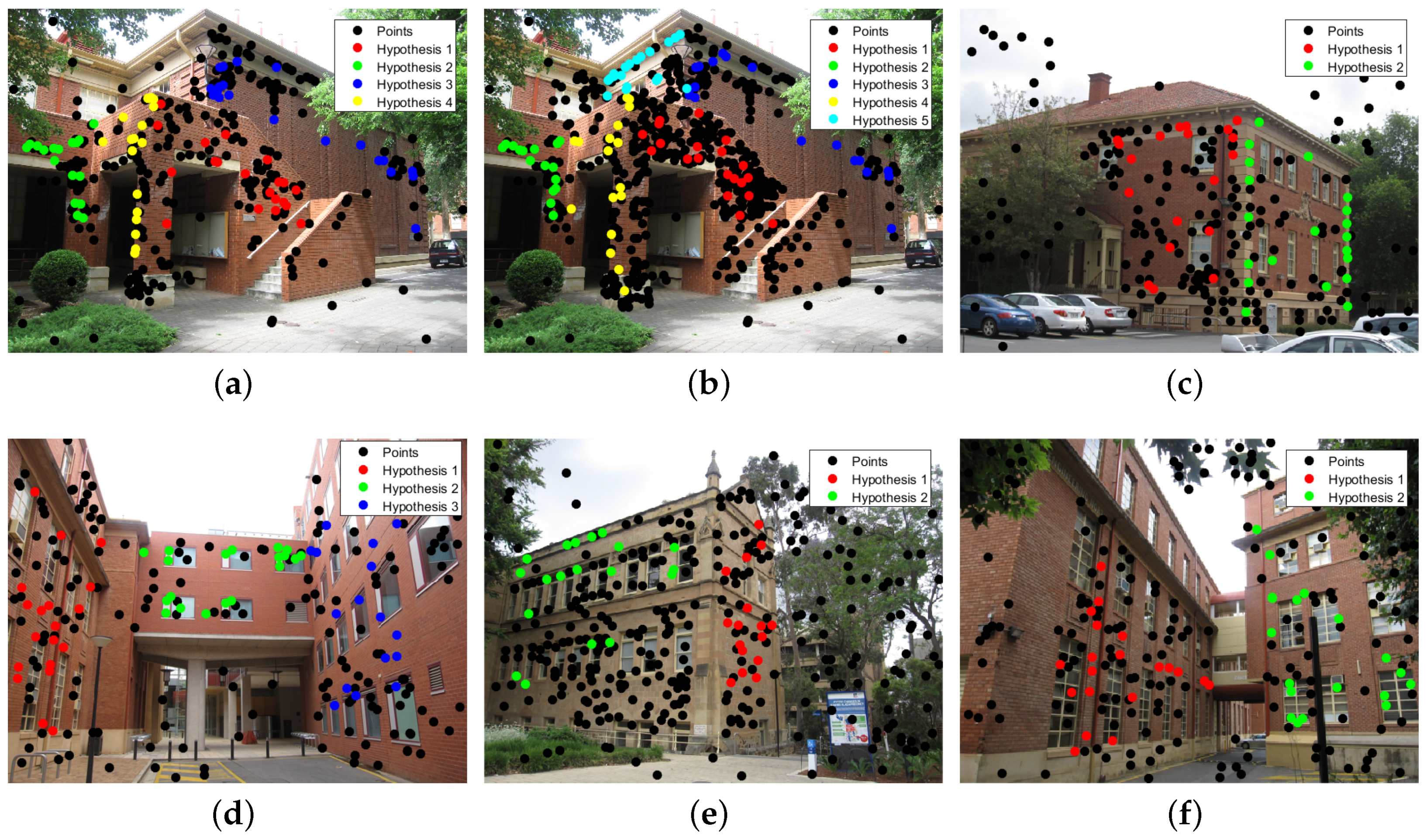
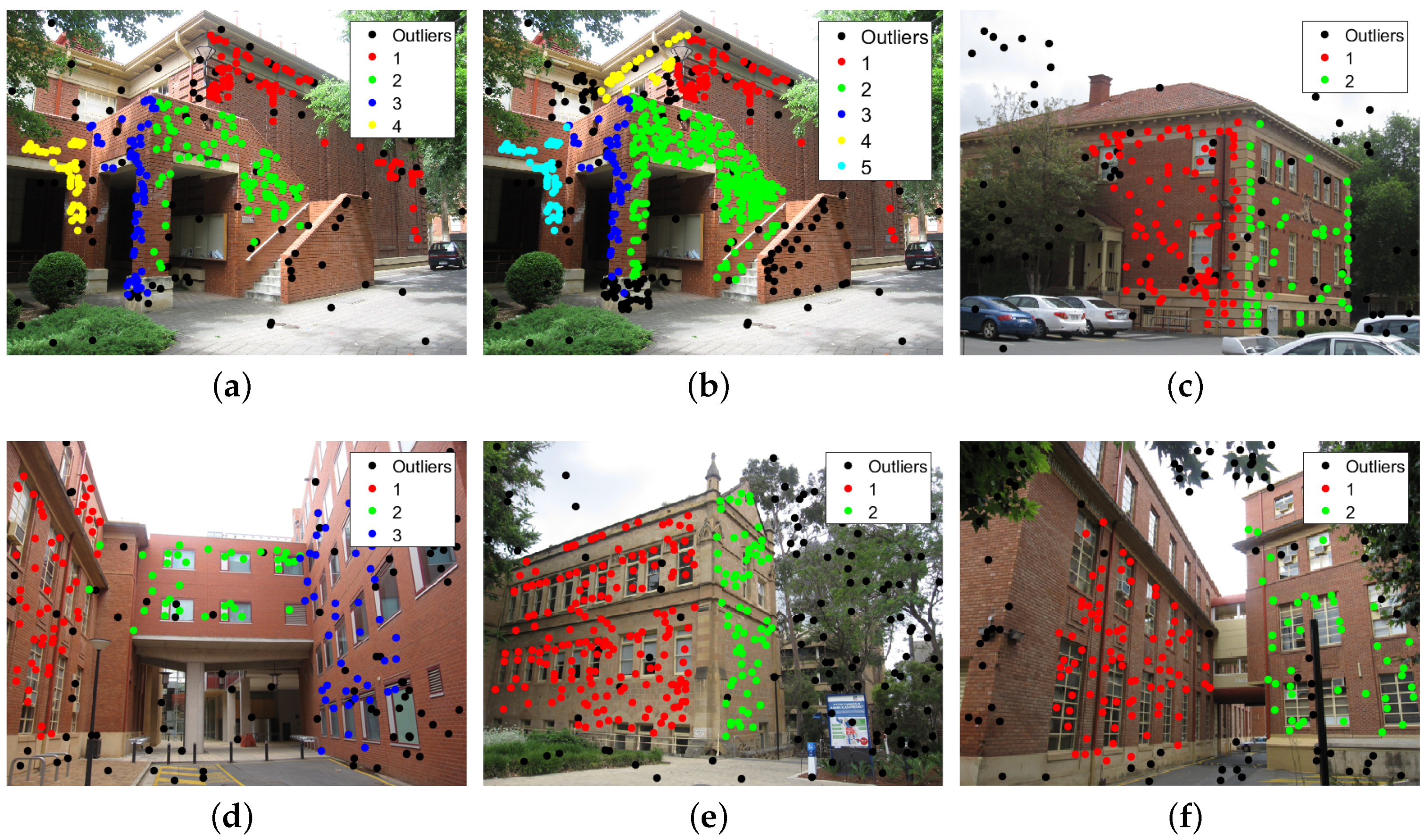
3.2. Multi-Fundamental Matrix Estimation
3.3. Computational Time Analysis
3.4. Computational Complexity Analysis
4. Conclusions
Author Contributions
Funding
Conflicts of Interest
References
- Fischler, M.A.; Bolles, R.C. Random sample consensus: A paradigm for model fitting with applications to image analysis and automated cartography. Commun. ACM 1981, 24, 381–395. [Google Scholar] [CrossRef]
- Stewart, C.V. Bias in robust estimation caused by discontinuities and multiple structures. IEEE Trans. Pattern Anal. Mach. Intell. 1997, 19, 818–833. [Google Scholar] [CrossRef]
- Vincent, E.; Laganiére, R. Detecting planar homographies in an image pair. In Proceedings of the 2nd International Symposium on Image and Signal Processing and Analysis, Pula, Croatia, 19–21 July 2001; pp. 182–187. [Google Scholar]
- Kanazawa, Y.; Kawakami, H. Detection of Planar Regions with Uncalibrated Stereo Using Distributions of Feature Points. BMVC. Citeseer. 2004, pp. 1–10. Available online: https://pdfs.semanticscholar.org/eb64/33aec14122d1805000c0f7d8ebc79eb73f54.pdf (accessed on 24 June 2020).
- Zuliani, M.; Kenney, C.S.; Manjunath, B. The multiransac algorithm and its application to detect planar homographies. In Proceedings of the IEEE International Conference on Image Processing 2005, Genoa, Italy, 11–14 September 2005; Volume 3, p. III-153. [Google Scholar]
- Pham, T.T.; Chin, T.J.; Yu, J.; Suter, D. Simultaneous sampling and multi-structure fitting with adaptive reversible jump mcmc. In Advances in Neural Information Processing Systems; MIT Press: Cambridge, MA, USA, 2011; pp. 540–548. [Google Scholar]
- Xu, L.; Oja, E.; Kultanen, P. A new curve detection method: Randomized Hough transform (RHT). Pattern Recognit. Lett. 1990, 11, 331–338. [Google Scholar] [CrossRef]
- Zhang, W.; Kǒsecká, J. Nonparametric estimation of multiple structures with outliers. In Dynamical Vision; Springer: Berlin, Germany, 2007; pp. 60–74. [Google Scholar]
- Comaniciu, D.; Meer, P. Mean shift: A robust approach toward feature space analysis. IEEE Trans. Pattern Anal. Mach. Intell. 2002, 24, 603–619. [Google Scholar] [CrossRef]
- Subbarao, R.; Meer, P. Nonlinear mean shift over Riemannian manifolds. Int. J. Comput. Vis. 2009, 84, 1–20. [Google Scholar] [CrossRef]
- Magri, L.; Fusiello, A. Robust Multiple Model Fitting with Preference Analysis and Low-rank Approximation. In Proceedings of the British Machine Vision Conference, Swansea, UK, 7–10 September 2015. [Google Scholar]
- Toldo, R.; Fusiello, A. Robust multiple structures estimation with j-linkage. In Proceedings of the European Conference on Computer Vision, Marseille, France, 12–18 September 2008; pp. 537–547. [Google Scholar]
- Toldo, R.; Fusiello, A. Real-time incremental j-linkage for robust multiple structures estimation. In Proceedings of the International Symposium on 3D Data Processing, Visualization and Transmission (3DPVT), Paris, France, 17–20 May 2010; Volume 1, p. 6. [Google Scholar]
- Magri, L.; Fusiello, A. T-linkage: A continuous relaxation of j-linkage for multi-model fitting. In Proceedings of the IEEE Conference on Computer Vision and Pattern Recognition, Columbus, OH, USA, 23–28 June 2014; pp. 3954–3961. [Google Scholar]
- Magri, L.; Fusiello, A. Multiple Model Fitting as a Set Coverage Problem. In Proceedings of the IEEE Conference on Computer Vision and Pattern Recognition, Las Vegas, NV, USA, 26 June–1 July 2016; pp. 3318–3326. [Google Scholar]
- Chin, T.J.; Wang, H.; Suter, D. Robust fitting of multiple structures: The statistical learning approach. In Proceedings of the IEEE 12th International Conference on Computer Vision, Kyoto, Japan, 27 September–4 October 2009; pp. 413–420. [Google Scholar]
- Wang, H.; Chin, T.J.; Suter, D. Simultaneously fitting and segmenting multiple-structure data with outliers. IEEE Trans. Pattern Anal. Mach. Intell. 2012, 34, 1177–1192. [Google Scholar] [CrossRef] [PubMed]
- Isack, H.; Boykov, Y. Energy-based geometric multi-model fitting. Int. J. Comput. Vis. 2012, 97, 123–147. [Google Scholar] [CrossRef]
- Pham, T.T.; Chin, T.J.; Yu, J.; Suter, D. The random cluster model for robust geometric fitting. IEEE Trans. Pattern Anal. Mach. Intell. 2014, 36, 1658–1671. [Google Scholar] [CrossRef]
- Yu, J.; Chin, T.J.; Suter, D. A global optimization approach to robust multi-model fitting. In Proceedings of the IEEE Conference on Computer Vision and Pattern Recognition (CVPR), Long Beach, CA, USA, 16–20 June 2011; pp. 2041–2048. [Google Scholar]
- Pham, T.T.; Chin, T.J.; Schindler, K.; Suter, D. Interacting geometric priors for robust multimodel fitting. IEEE Trans. Image Process. 2014, 23, 4601–4610. [Google Scholar] [CrossRef]
- Amayo, P.; Piniés, P.; Paz, L.M.; Newman, P. Geometric Multi-Model Fitting with a Convex Relaxation Algorithm. arXiv 2017, arXiv:1706.01553. [Google Scholar]
- Wang, H.; Xiao, G.; Yan, Y.; Suter, D. Mode-seeking on hypergraphs for robust geometric model fitting. In Proceedings of the IEEE International Conference on Computer Vision, Las Condes, Chile, 11–18 December 2015; pp. 2902–2910. [Google Scholar]
- Xiao, G.; Wang, H.; Lai, T.; Suter, D. Hypergraph modelling for geometric model fitting. Pattern Recognit. 2016, 60, 748–760. [Google Scholar] [CrossRef]
- Wang, H.; Yan, Y.; Suter, D. Searching for Representative Modes on Hypergraphs for Robust Geometric Model Fitting. IEEE Trans. Pattern Anal. Mach. Intell. 2018. [Google Scholar] [CrossRef] [PubMed]
- Purkait, P.; Chin, T.J.; Sadri, A.; Suter, D. Clustering with hypergraphs: The case for large hyperedges. IEEE Trans. Pattern Anal. Mach. Intell. 2017, 39, 1697–1711. [Google Scholar] [CrossRef]
- Wong, H.S.; Chin, T.J.; Yu, J.; Suter, D. Mode seeking over permutations for rapid geometric model fitting. Pattern Recognit. 2013, 46, 257–271. [Google Scholar] [CrossRef]
- Wong, H.S.; Chin, T.J.; Yu, J.; Suter, D. A simultaneous sample-and-filter strategy for robust multi-structure model fitting. Comput. Vis. Image Underst. 2013, 117, 1755–1769. [Google Scholar] [CrossRef]
- Wang, H.; Suter, D. Robust adaptive-scale parametric model estimation for computer vision. IEEE Trans. Pattern Anal. Mach. Intell. 2004, 26, 1459–1474. [Google Scholar] [CrossRef] [PubMed]
- Lee, K.M.; Meer, P.; Park, R.H. Robust adaptive segmentation of range images. IEEE Trans. Pattern Anal. Mach. Intell. 1998, 20, 200–205. [Google Scholar]
- Bab-Hadiashar, A.; Suter, D. Robust segmentation of visual data using ranked unbiased scale estimate. Robotica 1999, 17, 649–660. [Google Scholar] [CrossRef]
- Lou, Z.; Gevers, T. Image Alignment by Piecewise Planar Region Matching. IEEE Trans. Multimed. 2014, 16, 2052–2061. [Google Scholar] [CrossRef]
- Song, Y.; Chen, X.; Wang, X.; Zhang, Y.; Li, J. 6-DOF Image Localization From Massive Geo-Tagged Reference Images. IEEE Trans. Multimed. 2016, 18, 1542–1554. [Google Scholar] [CrossRef]
- Wong, H.S.; Chin, T.J.; Yu, J.; Suter, D. Dynamic and hierarchical multi-structure geometric model fitting. In Proceedings of the IEEE International Conference on Computer Vision, Barcelona, Spain, 7 November 2011; pp. 1044–1051. [Google Scholar]
- Mittal, S.; Anand, S.; Meer, P. Generalized projection-based M-estimator. IEEE Trans. Pattern Anal. Mach. Intell. 2012, 34, 2351–2364. [Google Scholar] [CrossRef] [PubMed]


| Methods | PEARL | J-Linkage | T-Linkage | SA-RCM | Proposed |
|---|---|---|---|---|---|
| johnsona | 4.02 | 5.07 | 4.02 | 5.90 | 5.09 |
| johnsonb | 18.18 | 18.33 | 18.33 | 17.95 | 14.18 |
| ladysymon | 5.49 | 9.25 | 5.06 | 7.17 | 1.69 |
| neem | 5.39 | 3.73 | 3.73 | 5.81 | 4.15 |
| oldclassicswing | 1.58 | 0.27 | 0.26 | 2.11 | 0.79 |
| sene | 0.80 | 0.84 | 0.40 | 0.80 | 0.40 |
| Methods | PEARL | J-Linkage | T-Linkage | SA-RCM | Proposed |
|---|---|---|---|---|---|
| biscuitbookbox | 4.25 | 1.55 | 1.54 | 7.04 | 0 |
| breadcartoychips | 5.91 | 11.26 | 3.37 | 4.81 | 0.84 |
| breadcubechips | 4.78 | 3.04 | 0.86 | 7.85 | 0.87 |
| breadtoycar | 6.63 | 5.49 | 4.21 | 3.82 | 1.20 |
| carchipscube | 11.82 | 4.27 | 1.81 | 11.75 | 0 |
| dinobooks | 14.72 | 17.11 | 9.44 | 8.03 | 7.22 |
| Scene | Points | Models | Outlier Rate (%) | Methods | Number of Samples | Computational Times (ms) |
|---|---|---|---|---|---|---|
| johnsona | 373 | 4 | 20.91 | T-Linkage | 2000 | 346 |
| Ours | 950 | 473 | ||||
| johnsonb | 649 | 7 | 12.02 | T-Linkage | 4000 | 977 |
| Ours | 1650 | 953 | ||||
| ladysymon | 237 | 2 | 32.49 | T-Linkage | 2000 | 249 |
| Ours | 600 | 284 | ||||
| neem | 241 | 3 | 36.51 | T-Linkage | 2000 | 281 |
| Ours | 600 | 305 | ||||
| oldclassicswing | 379 | 2 | 32.45 | T-Linkage | 2000 | 322 |
| Ours | 950 | 387 | ||||
| sene | 250 | 2 | 47.2 | T-Linkage | 2000 | 293 |
| Ours | 650 | 314 |
| Scene | Points | Models | Outlier Rate (%) | Methods | Number of Samples | Computational Times (ms) |
|---|---|---|---|---|---|---|
| biscuitbookbox | 259 | 3 | 37.45 | T-Linkage | 2000 | 305 |
| Ours | 1040 | 463 | ||||
| breadcartoychip | 237 | 4 | 34.6 | T-Linkage | 2000 | 287 |
| Ours | 960 | 431 | ||||
| breadcubechips | 230 | 3 | 35.22 | T-Linkage | 2000 | 284 |
| Ours | 960 | 405 | ||||
| breadtoycar | 166 | 3 | 33.73 | T-Linkage | 2000 | 213 |
| Ours | 720 | 316 | ||||
| carchipscube | 165 | 3 | 36.36 | T-Linkage | 2000 | 204 |
| Ours | 720 | 313 | ||||
| dinobooks | 360 | 3 | 43.06 | T-Linkage | 2000 | 473 |
| Ours | 1440 | 549 |
© 2020 by the authors. Licensee MDPI, Basel, Switzerland. This article is an open access article distributed under the terms and conditions of the Creative Commons Attribution (CC BY) license (http://creativecommons.org/licenses/by/4.0/).
Share and Cite
Zhao, Q.; Zhang, Y.; Qin, Q.; Luo, B. Quantized Residual Preference Based Linkage Clustering for Model Selection and Inlier Segmentation in Geometric Multi-Model Fitting. Sensors 2020, 20, 3806. https://doi.org/10.3390/s20133806
Zhao Q, Zhang Y, Qin Q, Luo B. Quantized Residual Preference Based Linkage Clustering for Model Selection and Inlier Segmentation in Geometric Multi-Model Fitting. Sensors. 2020; 20(13):3806. https://doi.org/10.3390/s20133806
Chicago/Turabian StyleZhao, Qing, Yun Zhang, Qianqing Qin, and Bin Luo. 2020. "Quantized Residual Preference Based Linkage Clustering for Model Selection and Inlier Segmentation in Geometric Multi-Model Fitting" Sensors 20, no. 13: 3806. https://doi.org/10.3390/s20133806
APA StyleZhao, Q., Zhang, Y., Qin, Q., & Luo, B. (2020). Quantized Residual Preference Based Linkage Clustering for Model Selection and Inlier Segmentation in Geometric Multi-Model Fitting. Sensors, 20(13), 3806. https://doi.org/10.3390/s20133806