A Novel Link-to-System Mapping Technique Based on Machine Learning for 5G/IoT Wireless Networks


Abstract
:1. Introduction
- (1)
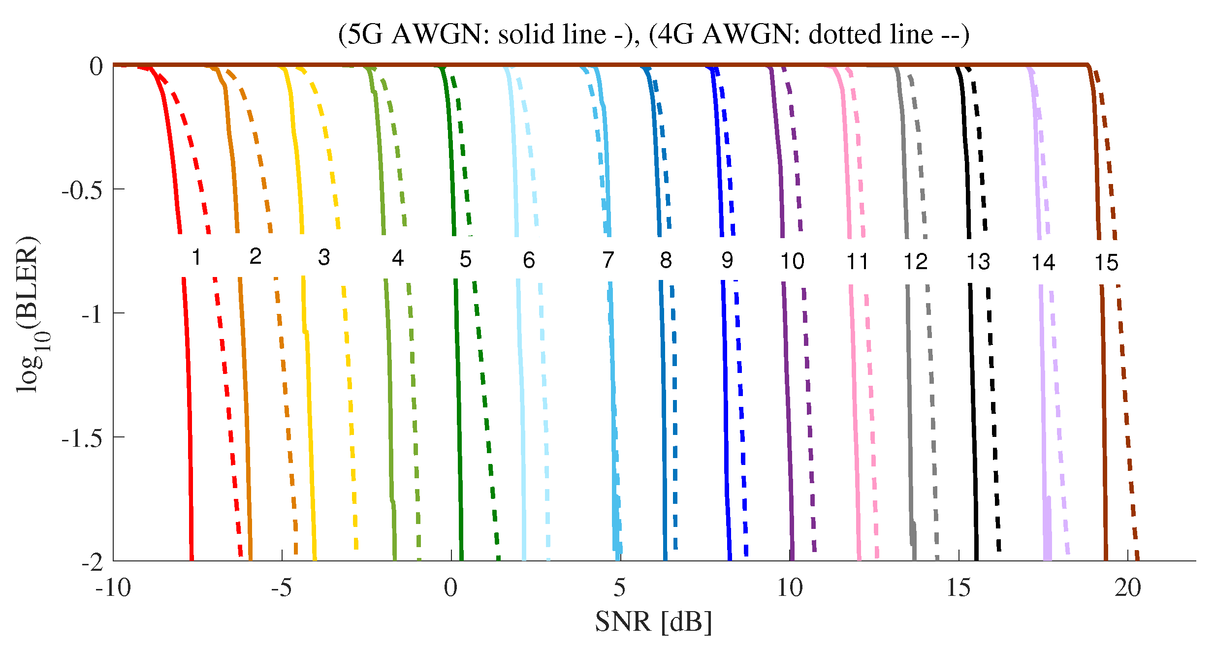
- AWGN curves based on 5G NR system are provided. In conventional L2S mapping schemes, an AWGN curve is required to estimate block error rate (BLER) on SLS. We provide the AWGN curve of SNR-BLER under 5G NR systems and compare the AWGN curves of SNR-BLER between 4G LTE system and 5G NR systems.
- (2)
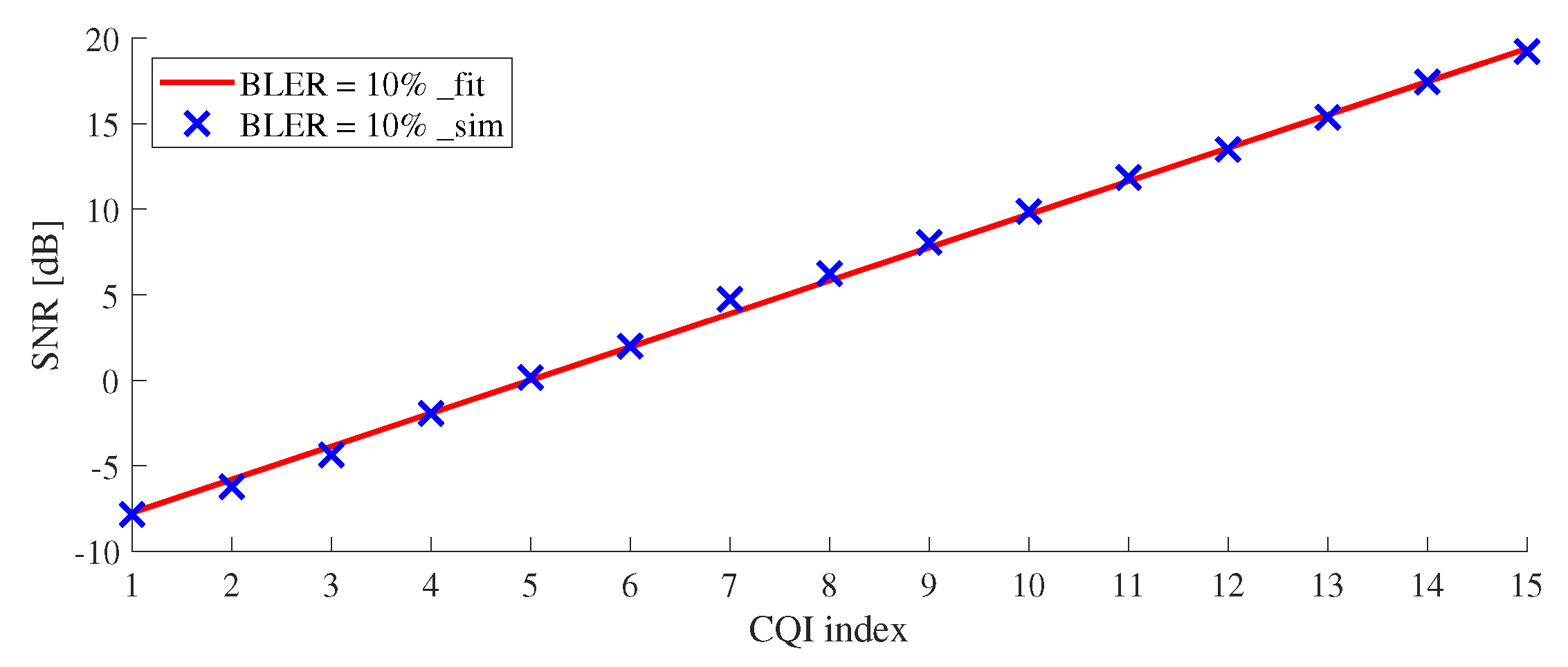
- The values of SNR satisfying at a target BLER = 0.1 (10%) are provided through AWGN curve. 3GPP 4G LTE and 5G NR-standards are specified to set the target BLER of 0.1, i.e., 10%. In SLS, signal-to noise ratio (SNR) can be measured immediately, but the calculation of BLER is burden because CRC decoding has to be performed. When a measured BLER is lower than the target BLER, UE can change to the index of higher CQI to support high data rate. Therefore, we provide the values of SNR thresholds under an unknown BLER satisfying the target BLER of 0.1 through the simulation results.
- (3)
- The methodology for 5G NR L2S mapping is provided based on ML. The optimal parameters for L2S mapping depend on a given environment. In addition, 5G NR systems have flexible frame structures. Therefore, we provide the methodology for 5G NR L2S mapping based on ML to extract the data for any cases and find the optimal mapping parameters.
- (4)
- The optimal mapping parameters for L2S mapping are provided in SISO and 2 × 2 MIMO cases under given conditions.
2. Background on 5G NR
3. Methodology for 5G NR Link-to-System Mapping
3.1. System Configuration/Setup
- (1)
- Waveform: Although several candidate waveforms for uplink were proposed, Rel-15 recently decided to use OFDM-based waveforms with cyclic prefix for 5G NR downlink and uplink.
- (2)
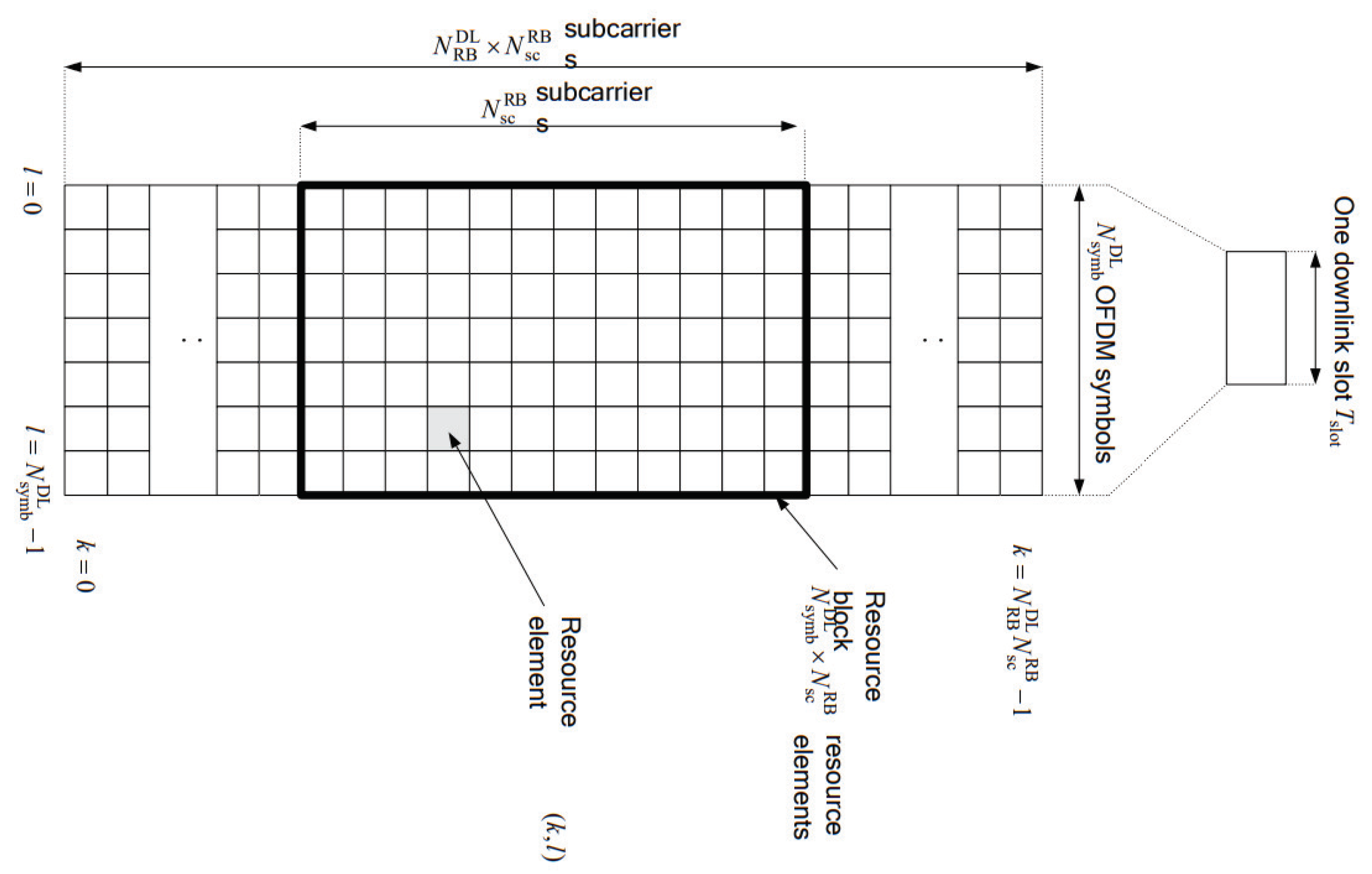
- Bandwidth and sub-carrier spacing: The size of resource blocks (RBs) is determined by the product of the number of sub-carriers on the frequency-axis and the number of symbols on the time-axis, as shown in Figure 1 [21]. Bandwidth is set to 5 MHz in this paper. The maximum number of available RBs is 25 at bandwidth of 5 MHz. When sub-carrier spacing is applied to 15 kHz, 12 sub-carriers are allocated in one RB on the frequency-axis and 14 symbols are allocated per sub-frame on the time-axis. A sub-frame consists of two slots and one slot consists of seven symbols. Assuming that the full band of 5 MHz is assigned to UE, 4200 resource elements (REs) can be allocated to UE for one sub-frame since 4200 REs are calculated by 25 RBs × 12 sub-carriers × 7 symbols × 2 slots per sub-frame. In other words, one RE is equivalent to the minimum resource for a symbol time on the time-axis and a sub-carrier on the frequency-axis.
- (3)
- Channel coding: 5G NR replaces the previously used Turbo-code to LDPC coding. The number of the information bits and the number of the encoded bit are varied depending on channel coding schemes, the number of RBs, and the modulation scheme. TB size represents the number of information bits that can be transmitted throughout 4200 REs and it is denoted as A. After encoding TB of length A by channel coding scheme, the output is to be encoded bits of length E. Table 3 summarizes values of A and E according to the turbo code and LDPC when using 25 RBs per sub-frame. denotes modulation order and its values are 2, 4, and 6 for QPSK, 16QAM, and 64QAM, respectively.
- (4)
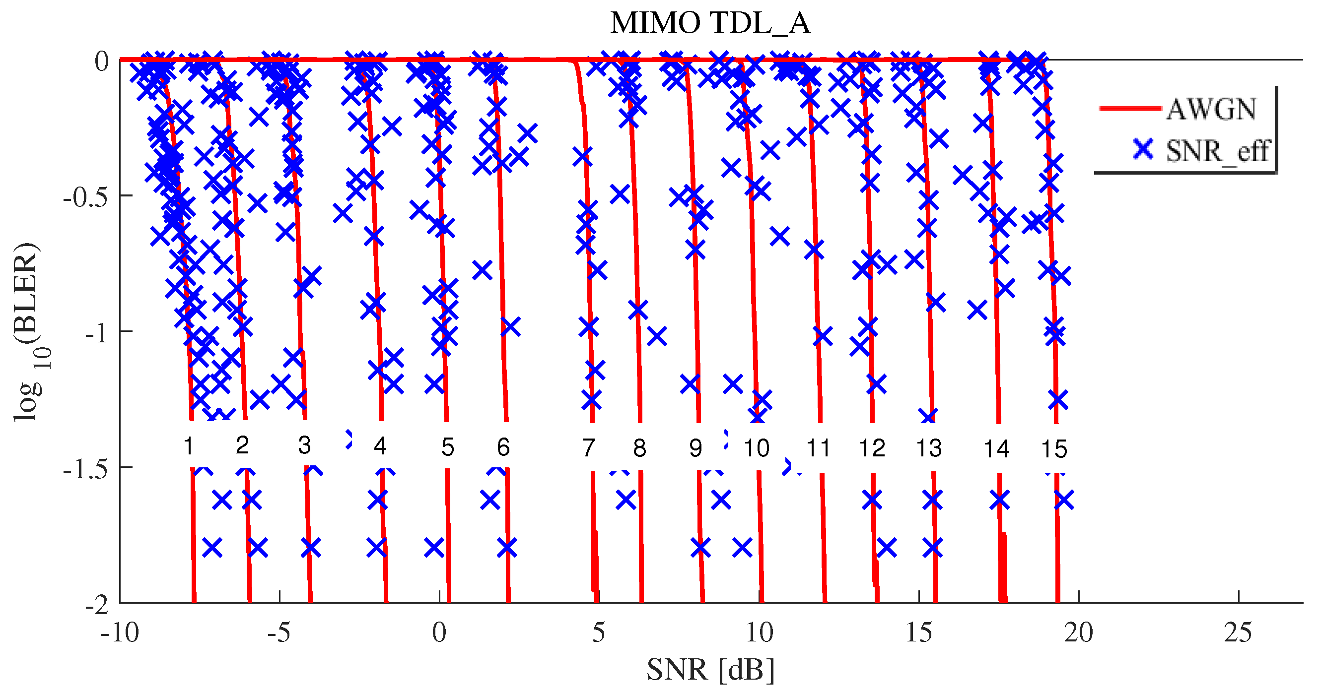
- Channel model: Ideally, transmit signal is transferred over AWGN channel after LDPC encoding and rate matching. In practice, we experimented with fading channel environments in which CDL-A and TDL-A are utilized in SISO and 2 × 2 MIMO environments.
3.2. Preliminary Phase for 5G NR L2S Mapping
3.3. Schematic of 5G NR L2S Mapping
- (1)
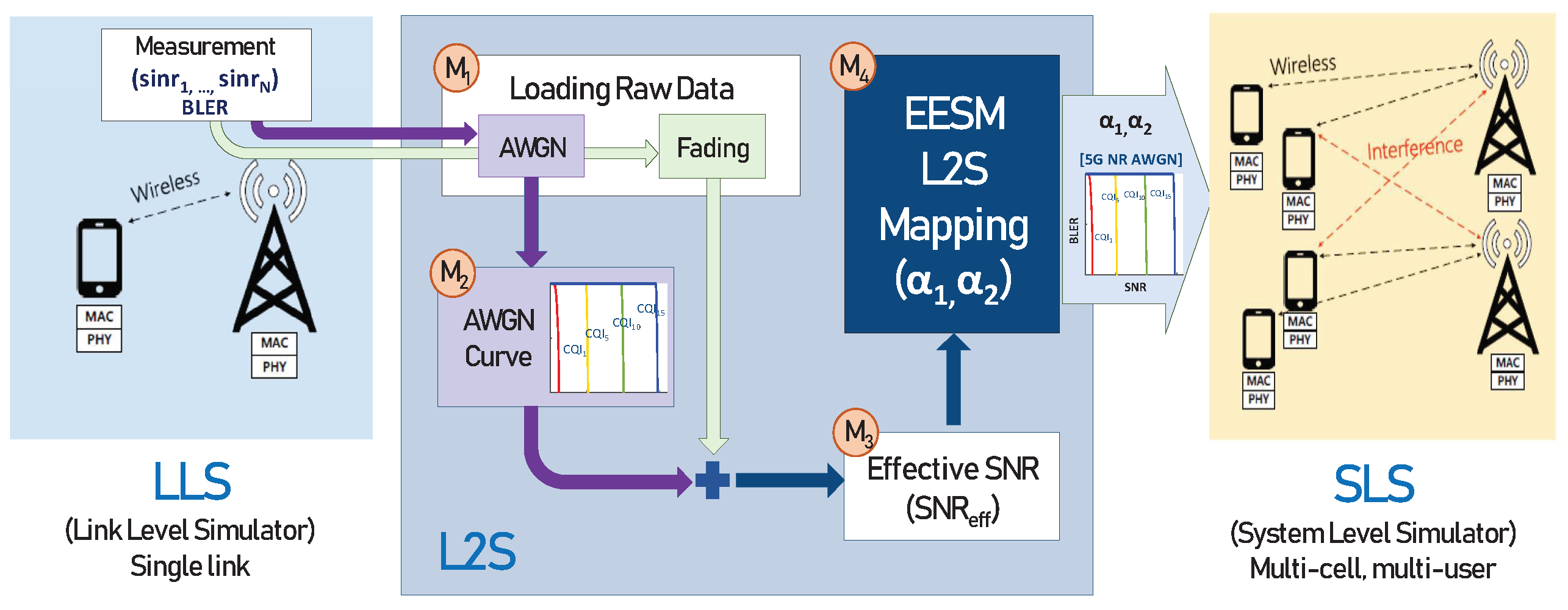
- Module : Loading raw datamodule reads stored data on the preliminary phase in Section 3.2. The format of raw data is composed of x rows and y columns for each CQI. The value of x is the number of input × the number of simulations () and the value of y is +2. As mentioned in Section 3.1, the number of allocated sub-carriers per sub-frame is . The first column is a given input SNR, the last column is , and the rest of columns mean , ⋯, . The data loading is performed for AWGN channel and all fading channels, respectively.
- (2)
- Module : AWGN curvemodule only applies to AWGN channel. It gets AWGN raw data from module and makes AWGN fitting curve for SNR versus BLER in the range of all CQIs. The AWGN fitting curve is generated from the relation of (, ⋯, ) and . Generally, the fitting curve is induced from an exponential function or regression curve of machine learning.
- (3)
- Module: Effective SNRmodule calculates an effective SNR applying and when a UE measures , and it is expressed as follows [5,6]:where and are determined after optimization in .In fact, SLS only measures without decoding. To estimate error for a received TB, SLS calculates an effective SNR from Equation (8) using and . The values of and are already reported to SLS through a L2S mapping method.
- (4)
- Module : EESM based L2S Mappingmodule finds optimal mapping parameters of and for a given CQI and a channel type. After performing M snapshots, we calculate mean square error (MSE) as follows [5,6]:where M denotes the total number of simulated snapshots and denotes the BLER measured from the ith post-processing SINR values. In addition, is calculated by Equation (8) at the ith snapshot, and is the value of BLER on AWGN channel. Furthermore, denotes output corresponding to input x from AWGN fitting curve. (It is plotted in module )To find optimal and , we minimize MSE for the entire range of (, ) as follows:Since the BLERs vs. SNR varies depending on the modulation method, code block size and code rate, we should find and for a given condition.
| Algorithm 1: Extract raw data. |
 |
4. Machine Learning Based Effective SNR Mapping Procedure
- (1)
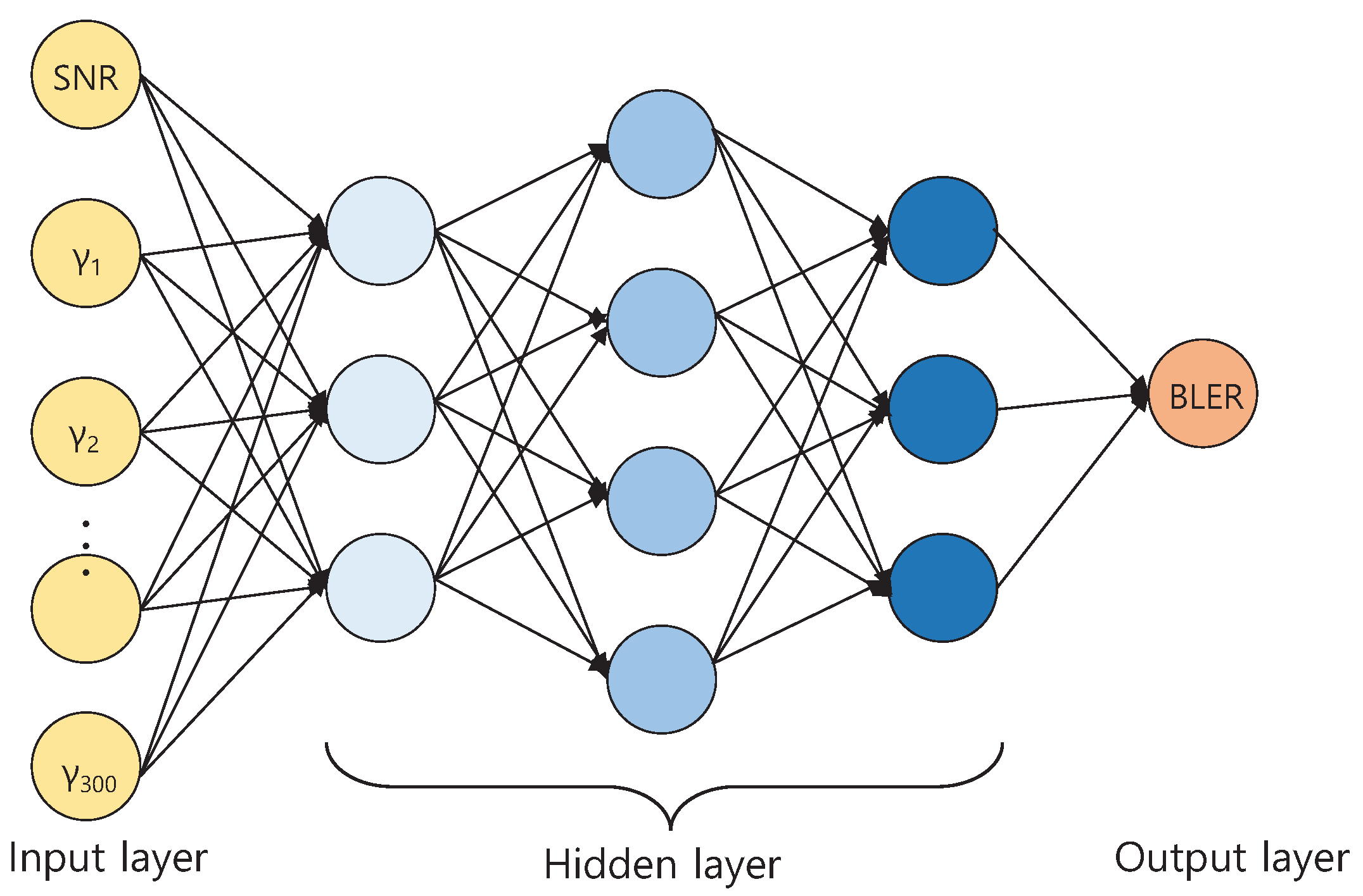
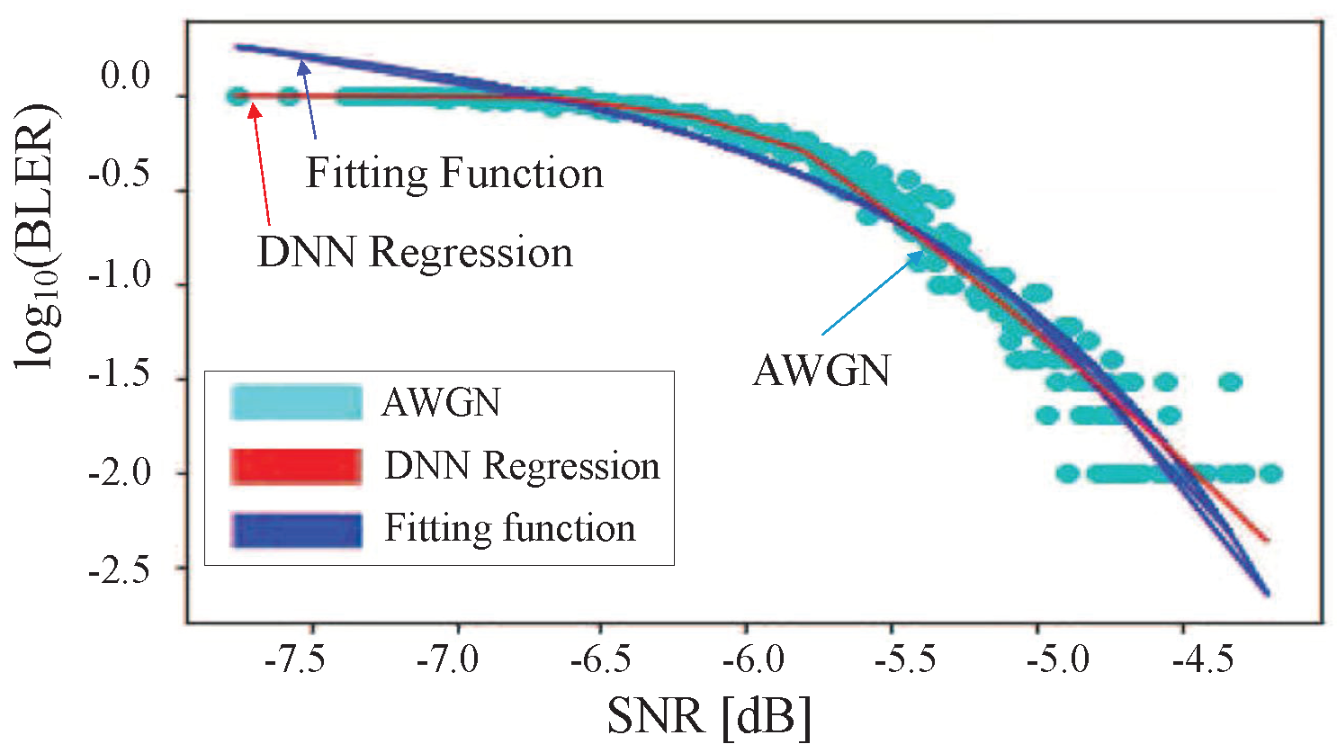
- We utilized the DNN regression method instead of the best fitting curve to obtain the BLER curve in AWGN channels. The DNN consists of several hidden layers between the input and output layers. Hidden layers of (100, 200, 100) layers were used in Adagrad optimizer [22]. As the number of hidden layers and the number of nodes at each hidden layer increased, MSE decreased. However, the improvement of MSE was saturated at three hidden layers with the number of nodes of (100, 200, 100), as shown in Figure 3. Learning rate was set to , which implies how quickly it is tuned to the target SNR value. The regularization strength to prevent over-fitting was set to . The sigmoid function was used as an activation function in hidden layers.
- (2)
- DNN regression continued training for SNRs and BLERs on AWGN channel with the learning rate at each epoch. The number of training data was 4000.
- (3)
- After training data, BLERs were predicted for test set of SNRs. Finally, we obtained an enhanced AWGN curve of SNRs and BLERs.
| Algorithm 2: DNN regression. |
| /* Configure DNN regression */ 1 regressor = learn.DNNRegressor(feature_columns, hidden_units = [100, 200, 100], optimizer = tf.train.ProximalAdagradOptimizer( learning_rate = 0.1, l1_regularization_strength = 0.001), activation_fn = tf.nn.sigmoid) /* Train measured data up to 4000 times */ 2 input_training_fn ← (awgn_snr, awgn_bler) 3 regressor.fit(input_fn = input_training_fn, steps = 4000) /* Predict of BLERs for test SNRs */ 4 input_reff_fn ← snr range 5 predictions = list(regressor.predict_scores(input_fn = input_reff_fn)) 6 regressed_bler = np.asarray(predictions) |
- (1)
- To find the optimal parameters , we loaded raw data from module in Section 3.2.
- (2)
- In the ML scheme, the loss function is defined as the difference between the calculated effective SNR value from Algorithm 3 and AWGN SNR obtained from Algorithm 2 at the same BLER. We calculated loss as the expectation of loss function over BLERs. The loss function and MSE of Equation (9) were used almost synonymously.
- (3)
- We applied optimization algorithms, Adagrad and RMSProp, to find the optimal parameters that minimize the loss function. Since Adagrad and RMSProp adapt the learning rate to the parameters, they eliminate the need to manually tune the learning rate. Adagrad optimizer adapts the learning rates by scaling them inversely proportional to the sum of the historical squared values of the gradient. In contrast, RMSprop optimizer modifies AdaGrad for a nonconvex setting by changing gradient accumulation into exponentially weighted moving average [23].
- (4)
- With the optimal parameters, the mean squared error (MSE) was calculated by
| Algorithm 3: Find optimal and . |
| /* Load data on Fading channel ; */ 1 snr_k ← post-processing SINRs, bler ← BLER /* Calculate with and */ 2 snr_eff = -1 * alpha1 * tf.log(tf.reduce_mean (tf.exp(-1*snr_k/alpha2), axis = 1)) /* Decide target SNR by regression */ 3 target_snr ← predicted snr corresponding to BLER /* Calculate loss function */ 4 loss = tf.reduce_sum(tf.abs(tf.subtract (target_snr,snr_eff))) /* Select a training algorithm between Adagrad and RMSprop; Adagrad is selected in this case. */ 5 train = tf.train.AdagradOptimizer(0.1).minimize(loss) /* train = tf.train.RMSPropOptimizer(0.1).minimize(loss) ← when RMSProp is selected. */ /* Training data 4000 times */ 6 with tf.Session() as sess: 7 sess.run(init) 8 for i in range(4000): 9 sess.run(train) /* Calculate MSE in test data set */ 10 regressed_bler ← estimated BLER, y_data ← BLER 11 mse = np.mean(np.square(np.subtract(np.asarray(y_data), np.asarray(regressed_bler)))) |
5. Numerical Results and Analysis
5.1. AWGN Curve
5.2. Optimal Values of and
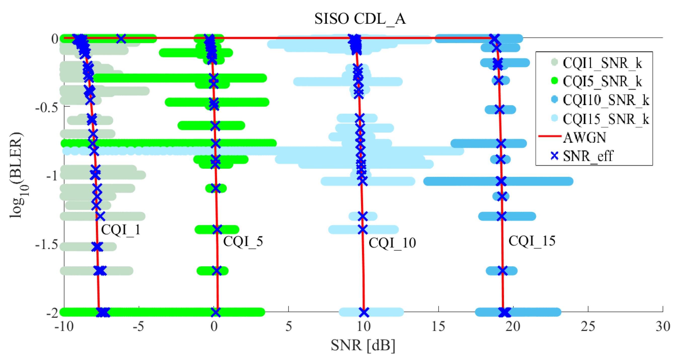
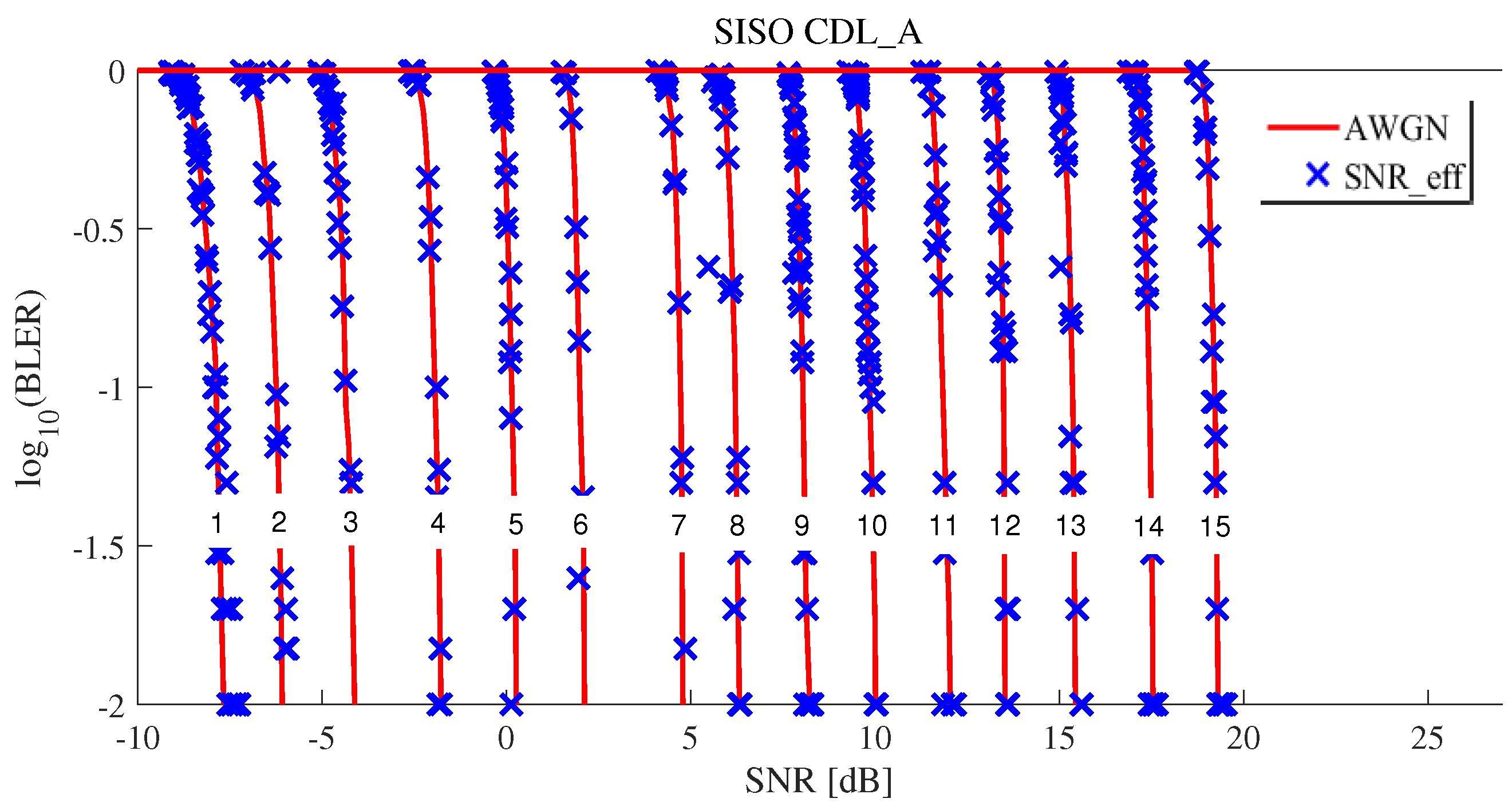
5.3. Simulation Validation
6. Conclusions
Author Contributions
Acknowledgments
Conflicts of Interest
References
- Chih-Lin, I.; Han, S.; Xu, Z.; Wang, S.; Sun, Q.; Chen, Y. New paradigm of 5G wireless internet. IEEE J. Sel. Areas Commun. 2016, 34, 474–482. [Google Scholar]
- ITU-R, Framework and Overall Objectives of the Future Development of IMT for 2020 and Beyond. Recommendations: M.2083. 2015. Available online: https://www.itu.int/rec/R-REC-M.2083-0-201509-I/en (accessed on 1 March 2019).
- Ding, Z.; Liu, Y.; Choi, J.; Sun, Q.; Elkashlan, M.; Poor, H.V. Application of non-orthogonal multiple access in LTE and 5G networks. IEEE Commun. Mag. 2017, 55, 185–191. [Google Scholar]
- Andrews, J.G. What will 5G be? IEEE J. Sel. Areas Commun. 2014, 32, 1065–1082. [Google Scholar] [CrossRef]
- Olmos, J.; Ruiz, S.; Gareia-Lozano, M.; Martin-Sacristan, D. Link Abstraction Models Based on Mutual Information for LTE Downlink; COST 2100 TD(10) 11052; iTEAM Research Institute: Aalborg, Denmark, 2010. [Google Scholar]
- Tuomaala, E.; Wang, H. Effective SINR approach of link to system mapping in OFDM/multi-carrier mobile network. In Proceedings of the IEEE the Second International Conference on Mobile Technology, Applications and Systems, Cape Town, South Africa, 15–17 November 2005; pp. 140–144. [Google Scholar]
- IEEE C802.16m-07097. Link Performance Abstraction Based on Mean Mutual Information Per Bit (MMIB) of the LLR Channel; IEEE 802.16 Broadband Wireless Access Working Group. 2007. Available online: http://www.wirelessman.org/tgm/contrib/C80216m-07_097.pdf (accessed on 1 March 2019).
- Hcine, M.B.; Bouallegue, R. Analysis of uplink effective SINR in LTE networks. In Proceedings of the 2015 International Wireless Communications and Mobile Computing Conference (IWCMC), Dubrovnik, Croatia, 24–28 August 2015. [Google Scholar]
- Hanzaz, Z.; Schotten, H.D. Impact of L2S interface on system level evaluation for LTE system. In Proceedings of the 2013 IEEE 11th Malaysia International Conference on Communications (MICC), Kuala Lumpur, Malaysia, 26–28 November 2013. [Google Scholar]
- Daniels, R.; Heath, R.W., Jr. Online adaptive modulation and coding with support vector machines. In Proceedings of the IEEE European Wireless Conference, Lucca, Italy, 12–15 April 2010; pp. 718–724. [Google Scholar]
- Mesa, A.C.; Aguayo-Torres, M.C.; Martin-Vega, F.J.; Gómez, G.; Blanquez-Casado, F.; Delgado-Luque, I.; Entrambasaguas, J. Link abstraction models for multicarrier systems: A logistic regression approach. Int. J. Commun. Syst. 2018, 31, e3436. [Google Scholar]
- Chu, E.; Jang, H.J.; Jung, B.C. Machine learning based link-to-system mapping for system-level simulation of cellular networks. In Proceedings of the 2018 Tenth International Conference on Ubiquitous and Future Networks, Prague, Czech Republic, 3–6 July 2018; pp. 503–506. [Google Scholar]
- Kim, Y.; Bae, J.; Lim, J.; Park, E.; Baek, J.; Han, S.I.; Han, Y. 5G K-Simulator: 5G System Simulator for Performance Evaluation. In Proceedings of the 2018 IEEE International Symposium on Dynamic Spectrum Access Networks (DySPAN), Seoul, Korea, 22–25 October 2018. [Google Scholar]
- Homepage of 5G K-Simulator. Available online: http://5gopenplatform.org/main/index.php (accessed on 1 March 2019).
- Berrou, C.; Glavieux, A.; Thitimajshima, P. Near Shannon limit error-correcting coding and decoding: Turbo codes. In Proceedings of the ICC ’93—IEEE International Conference on Communications, Geneva, Switzerland, 23–26 May 1993. [Google Scholar]
- MacKay, D.J.C.; Neal, R.M. Near Shannon limit performance of low density parity check codes. Electron. Lett. 1996, 32, 1645–1646. [Google Scholar] [CrossRef]
- Arikan, E. Channel polarization: A method for constructing capacity achieving codes for symmetric binary-input memoryless channels. IEEE Trans. Inf. Theory 2008, 55, 3051–3073. [Google Scholar] [CrossRef]
- 3rd Generation Partnership Project; Technical Specification Group Radio access Network (3GPP), TR 38.900 (V15.0.0), Study on Channel Model for Frequency Spectrum Above 6 GHz. July 2018. Available online: https://portal.3gpp.org/desktopmodules/Specifications/SpecificationDetails.aspx?specificationId=2991 (accessed on 1 March 2019).
- 3rd Generation Partnership Project; Technical Specification Group Radio access Network (3GPP), TR 38.901 (V15.0.0), Study on Channel Model for Frequency From 0.5 To 100 GHz. June 2018. Available online: https://portal.3gpp.org/desktopmodules/Specifications/SpecificationDetails.aspx?specificationId=3173 (accessed on 1 March 2019).
- 3rd Generation Partnership Project; Technical Specification Group Radio access Network (3GPP), TR 38.802 (V14.0.0), Study on New Radio Access Technology Physical Layer Aspects. March 2017. Available online: https://portal.3gpp.org/desktopmodules/Specifications/SpecificationDetails.aspx?specificationId=3066 (accessed on 1 March 2019).
- 3rd Generation Partnership Project; Technical Specification Group Radio access Network (3GPP), TS 38.211 (V15.3.0), Evolved Universal Terrestrial Radio Access (E-UTRA): Physical channels and modulation. 2018. Available online: https://portal.3gpp.org/desktopmodules/Specifications/SpecificationDetails.aspx?specificationId=3213 (accessed on 1 March 2018).
- Ruder, S. An overview of gradient descent optimization algorithms. arXiv, 2016; arXiv:1609.04747. [Google Scholar]
- Goodfellow, I.; Bengio, Y.; Courville, A.; Bach, F. Deep Learning (Adaptive Computation and Machine Learning Series); MIT Press: Cambridge, MA, USA, 2006. [Google Scholar]


| Abbreviation: Full Name | Abbreviation: Full Name |
|---|---|
| AWGN: additive white Gaussian noise | BLER: block error rate |
| CQI: channel quality indication | CDL: clustered delay line |
| DNN: deep neural network | EESM: exponential effective SNR mapping |
| eNB: evolved Node-B | LDPC: Low-density parity-check |
| LTE-A: long term evolution-advanced | LLS: link-level simulator |
| L2S: link-to-system | MIMO: multiple input multiple output |
| ML: machine learning | MMSE: minimum mean square error |
| MSE: mean squared error | NS: network-level simulator |
| NR: new radio | RB: resource block |
| RE: resource element | SINR: signal-to-interference plus noise ratio |
| SISO: single input single output | SLS: system-level simulator |
| SNR: signal-to-noise ratio | TB: transport block |
| TDL: tapped delay line | UE: user equipment |
| Parameters | Values |
|---|---|
| Waveform | OFDM |
| Carrier frequency | 2.8 GHz |
| Bandwidth | 5 MHz |
| Sub-carrier spacing | kHz |
| Channel Estimation | Perfect, MMSE |
| The number of allocated RBs to a UE | 25 RBs |
| The number of sub-carriers per RB | 12 sub-carriers |
| The number of symbols per slot | 7 symbols |
| The number of slots per sub-frame | 2 slots |
| Channel Coding | Turbo-Code (4G), LDPC (5G) |
| Channel Model | AWGN, CDL-A (SISO), TDL-A ( MIMO) |
| LDPC | Turbo Code | ||||||||
|---|---|---|---|---|---|---|---|---|---|
| CQI | Mod. | ||||||||
| [Bits] | [Bits] | × | [Bits] | [Bits] | × | ||||
| 1 | QPSK | 584 | 8000 | 0.0762 | 0.1523 | 608 | 7800 | 0.0779 | 0.1559 |
| 2 | QPSK | 912 | 8000 | 0.1172 | 0.2344 | 928 | 7800 | 0.1190 | 0.2379 |
| 3 | QPSK | 1480 | 8000 | 0.1885 | 0.3770 | 1480 | 7800 | 0.1897 | 0.3795 |
| 4 | QPSK | 2384 | 8000 | 0.3008 | 0.6016 | 2408 | 7800 | 0.3087 | 0.6174 |
| 5 | QPSK | 3480 | 8000 | 0.4385 | 0.8770 | 3496 | 7800 | 0.4482 | 0.8964 |
| 6 | QPSK | 4680 | 8000 | 0.5879 | 1.1758 | 4608 | 7800 | 0.5908 | 1.1815 |
| 7 | 16QAM | 5880 | 16,000 | 0.3691 | 1.4766 | 5760 | 15,600 | 0.3692 | 1.4769 |
| 8 | 16QAM | 7632 | 16,000 | 0.4785 | 1.9141 | 7424 | 15,600 | 0.4759 | 1.9036 |
| 9 | 16QAM | 9600 | 16,000 | 0.6016 | 2.4063 | 9480 | 15,600 | 0.6077 | 2.4308 |
| 10 | 64QAM | 10,896 | 24,000 | 0.4551 | 2.7305 | 10,760 | 23,400 | 0.4598 | 2.7590 |
| 11 | 64QAM | 13,264 | 24,000 | 0.5537 | 3.3223 | 13,064 | 23,400 | 0.5583 | 3.3497 |
| 12 | 64QAM | 15,584 | 24,000 | 0.6504 | 3.9023 | 15,112 | 23,400 | 0.6458 | 3.8749 |
| 13 | 64QAM | 18,072 | 24,000 | 0.7539 | 4.5234 | 17,424 | 23,400 | 0.7446 | 4.4677 |
| 14 | 64QAM | 20,440 | 24,000 | 0.8525 | 5.1152 | 19,968 | 23,400 | 0.8533 | 5.1200 |
| 15 | 64QAM | 22,192 | 24,000 | 0.9258 | 5.5547 | 21,504 | 23,400 | 0.9190 | 5.5138 |
| CQI Index | CQI 1 | CQI 2 | CQI 3 | CQI 4 | CQI 5 | CQI 6 | CQI 7 | CQI 8 |
|---|---|---|---|---|---|---|---|---|
| FIT | 0.033 | 0.027 | 0.033 | 0.038 | 0.017 | 0.032 | 0.017 | 0.012 |
| DNN | 0.018 | 0.014 | 0.016 | 0.013 | 0.014 | 0.011 | 0.015 | 0.016 |
| CQI Index | CQI 9 | CQI 10 | CQI 11 | CQI 12 | CQI 13 | CQI 14 | CQI 15 | - |
| FIT | 0.019 | 0.021 | 0.011 | 0.025 | 0.013 | 0.015 | 0.030 | - |
| DNN | 0.011 | 0.008 | 0.013 | 0.013 | 0.010 | 0.013 | 0.010 | - |
| CQI Index | CQI 1 | CQI 2 | CQI 3 | CQI 4 | CQI 5 | CQI 6 | CQI 7 | CQI 8 |
|---|---|---|---|---|---|---|---|---|
| SNR Threshold [dB] | −7.8474 | −6.2369 | −4.3591 | −1.9319 | 0.1509 | 1.9976 | 4.7278 | 6.2231 |
| CQI Index | CQI 9 | CQI 10 | CQI 11 | CQI 12 | CQI 13 | CQI 14 | CQI 15 | - |
| SNR Threshold [dB] | 8.0591 | 9.8585 | 11.8432 | 13.4893 | 15.3598 | 17.4435 | 19.2155 | - |
| CQI | AdaGrad | RMSProp | |||||
|---|---|---|---|---|---|---|---|
| MSE | MSE | ||||||
| 1 | 3.294 | 3.230 | 0.150 | 2.752 | 2.698 | 0.149 | |
| 2 | 1.874 | 1.880 | 0.357 | 2.163 | 2.170 | 0.364 | |
| 3 | 1.607 | 1.594 | 0.065 | 2.002 | 1.988 | 0.061 | |
| 4 | 1.184 | 1.175 | 0.159 | 1.162 | 1.154 | 0.156 | |
| 5 | 1.286 | 1.283 | 0.140 | 1.552 | 1.546 | 0.206 | |
| 6 | 1.359 | 1.359 | 0.055 | 1.360 | 0.360 | 0.056 | |
| 7 | 3.642 | 3.628 | 0.170 | 3.643 | 3.629 | 0.170 | |
| 8 | 3.256 | 3.228 | 0.171 | 3.937 | 3.911 | 0.155 | |
| 9 | 5.563 | 5.543 | 0.110 | 5.636 | 5.616 | 0.110 | |
| 10 | 16.259 | 16.204 | 0.075 | 16.262 | 16.208 | 0.075 | |
| 11 | 13.685 | 13.604 | 0.329 | 13.382 | 13.301 | 0.268 | |
| 12 | 17.988 | 18.079 | 0.778 | 17.547 | 17.632 | 0.724 | |
| 13 | 23.971 | 23.970 | 0.555 | 24.112 | 24.111 | 0.558 | |
| 14 | 29.306 | 29.205 | 0.210 | 29.306 | 29.204 | 0.210 | |
| 15 | 33.590 | 33.833 | 0.533 | 28.733 | 28.739 | 0.823 | |
| CQI | AdaGrad | RMSProp | |||||
|---|---|---|---|---|---|---|---|
| MSE | MSE | ||||||
| 1 | 0.088 | 0.126 | 1.581 | 0.079 | 0.106 | 1.465 | |
| 2 | 0.114 | 0.154 | 0.834 | 0.114 | 0.152 | 0.969 | |
| 3 | 0.200 | 0.252 | 0.730 | 0.208 | 0.260 | 1.070 | |
| 4 | 0.280 | 0.306 | 0.867 | 0.301 | 0.339 | 0.976 | |
| 5 | 0.511 | 0.525 | 0.859 | 0.513 | 0.528 | 0.865 | |
| 6 | 0.718 | 0.729 | 2.072 | 0.718 | 0.729 | 2.070 | |
| 7 | 2.664 | 3.554 | 1.526 | 2.664 | 3.553 | 1.528 | |
| 8 | 2.465 | 2.665 | 1.538 | 2.465 | 2.664 | 1.525 | |
| 9 | 3.200 | 4.695 | 1.782 | 3.203 | 4.700 | 1.784 | |
| 10 | 6.532 | 8.174 | 1.824 | 6.338 | 7.900 | 1.777 | |
| 11 | 6.588 | 8.619 | 0.703 | 5.969 | 7.634 | 0.688 | |
| 12 | 9.985 | 11.538 | 1.125 | 10.021 | 11.661 | 1.135 | |
| 13 | 11.190 | 14.225 | 1.393 | 11.19 | 14.224 | 1.399 | |
| 14 | 15.933 | 19.071 | 0.973 | 19.562 | 23.828 | 2.784 | |
| 15 | 20.410 | 38.530 | 1.399 | 19.062 | 34.963 | 1.099 | |
© 2019 by the authors. Licensee MDPI, Basel, Switzerland. This article is an open access article distributed under the terms and conditions of the Creative Commons Attribution (CC BY) license (http://creativecommons.org/licenses/by/4.0/).
Share and Cite
Chu, E.; Yoon, J.; Jung, B.C. A Novel Link-to-System Mapping Technique Based on Machine Learning for 5G/IoT Wireless Networks. Sensors 2019, 19, 1196. https://doi.org/10.3390/s19051196
Chu E, Yoon J, Jung BC. A Novel Link-to-System Mapping Technique Based on Machine Learning for 5G/IoT Wireless Networks. Sensors. 2019; 19(5):1196. https://doi.org/10.3390/s19051196
Chicago/Turabian StyleChu, Eunmi, Janghyuk Yoon, and Bang Chul Jung. 2019. "A Novel Link-to-System Mapping Technique Based on Machine Learning for 5G/IoT Wireless Networks" Sensors 19, no. 5: 1196. https://doi.org/10.3390/s19051196
APA StyleChu, E., Yoon, J., & Jung, B. C. (2019). A Novel Link-to-System Mapping Technique Based on Machine Learning for 5G/IoT Wireless Networks. Sensors, 19(5), 1196. https://doi.org/10.3390/s19051196