Performance Evaluation of Non-GPS Based Localization Techniques under Shadowing Effects

 , ,
, ,  , and
, and
Abstract
1. Introduction
- review of the state-of-the art non-GPS localization techniques with the focus on RSSI and AOA methods;
- proposal of combined RSSI-AOA localization methods with different weights of the components RSSI and AOA;
- comprehensive summary on working concepts of these combined methods;
- introduction of the localization model under shadowing effects; and
- numerous simulations and in-depth discussions on the precision and accuracy of the proposed combined localization techniques under shadowing effects.
2. Related Works
2.1. Distance and Angle Estimation Concepts
2.1.1. RSSI
2.1.2. AOA
2.2. Existing Localization Methods
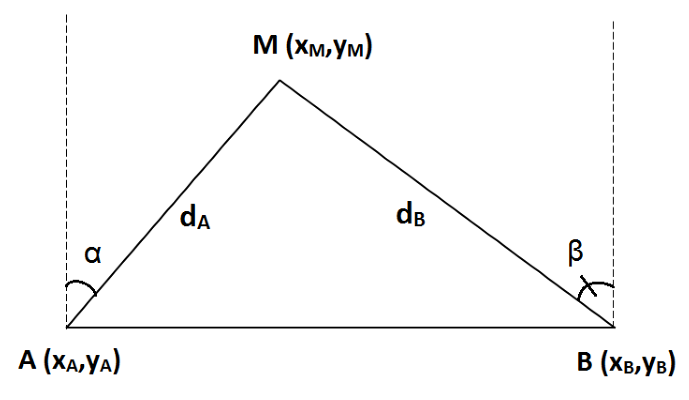
2.2.1. Triangulation (2AOA)
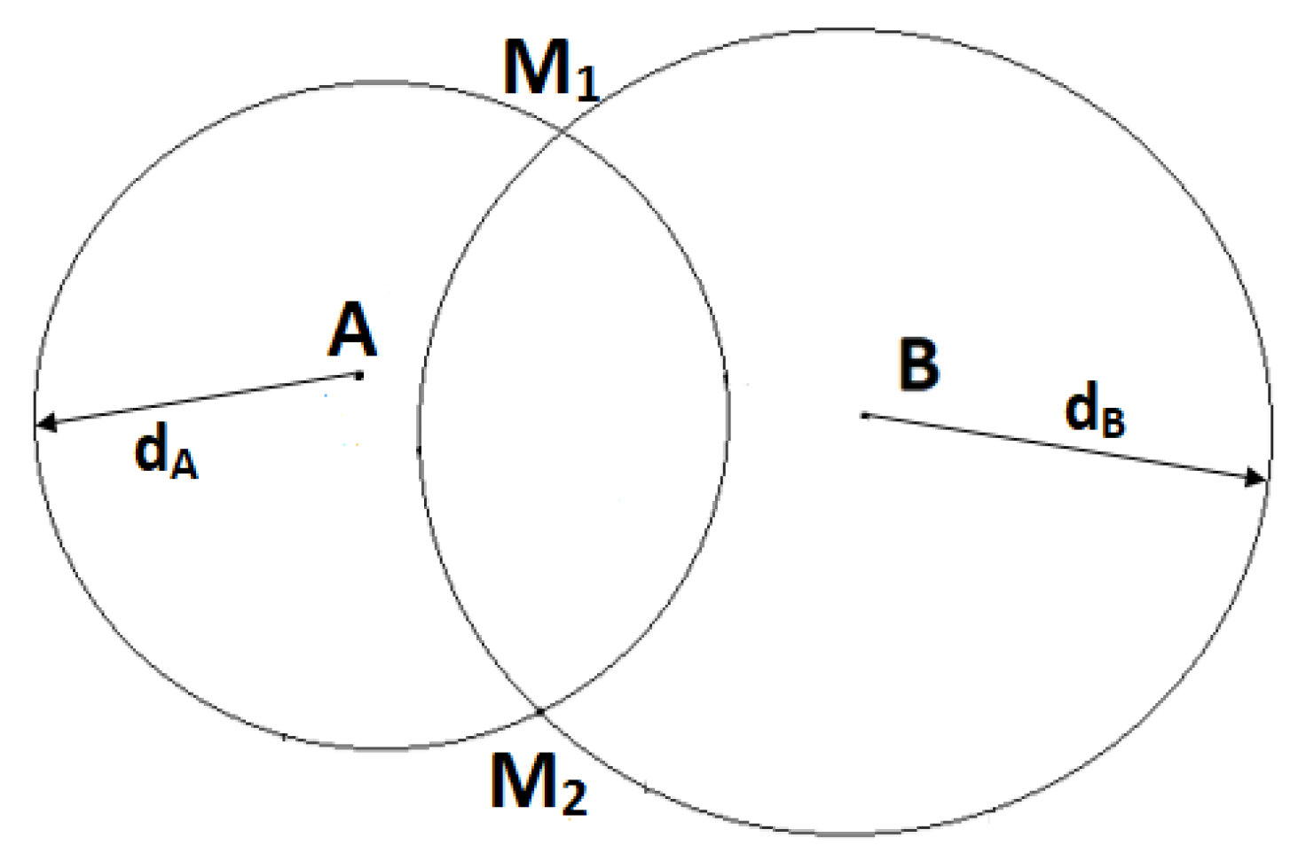
2.2.2. Trilateration with Two Anchors (2RSSI)
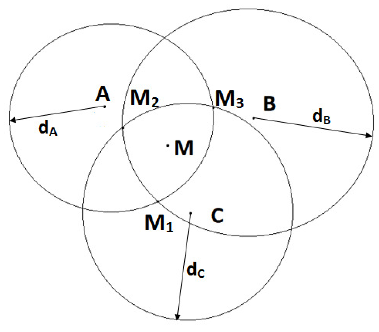
2.2.3. Trilateration with Three Anchors (3RSSI)
2.2.4. Weighted Centroid Method (weighted 3RSSI)
3. Localization Using Combinations of RSSI and AOA
3.1. 1AOA + 1RSSI
3.2. 1AOA + 2RSSI
3.3. 2AOA + 1RSSI
3.4. 2AOA + 2RSSI
4. Localization under Shadowing Effects
5. Simulation Results and Analyses
5.1. Precision
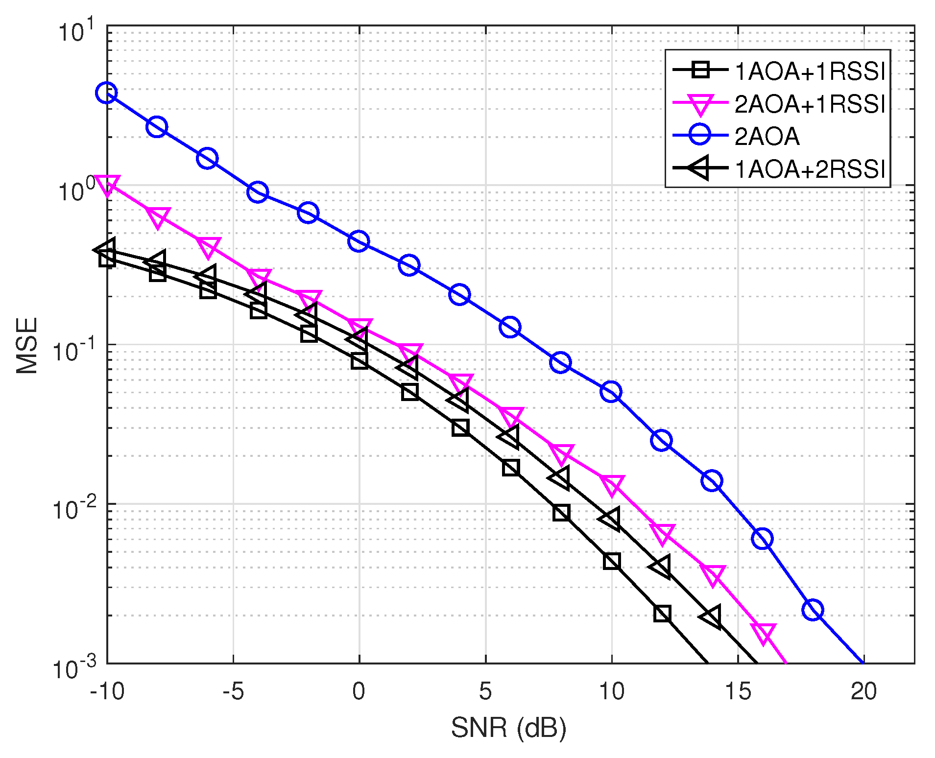
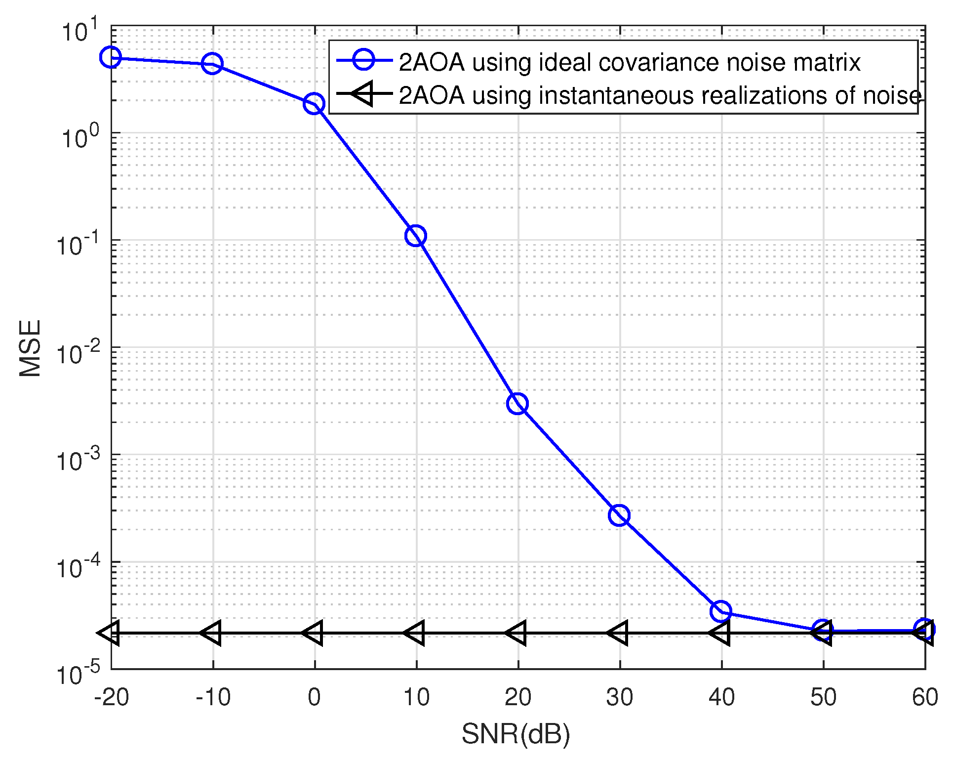
5.1.1. Localization with Ideal Covariance Matrix of Noise
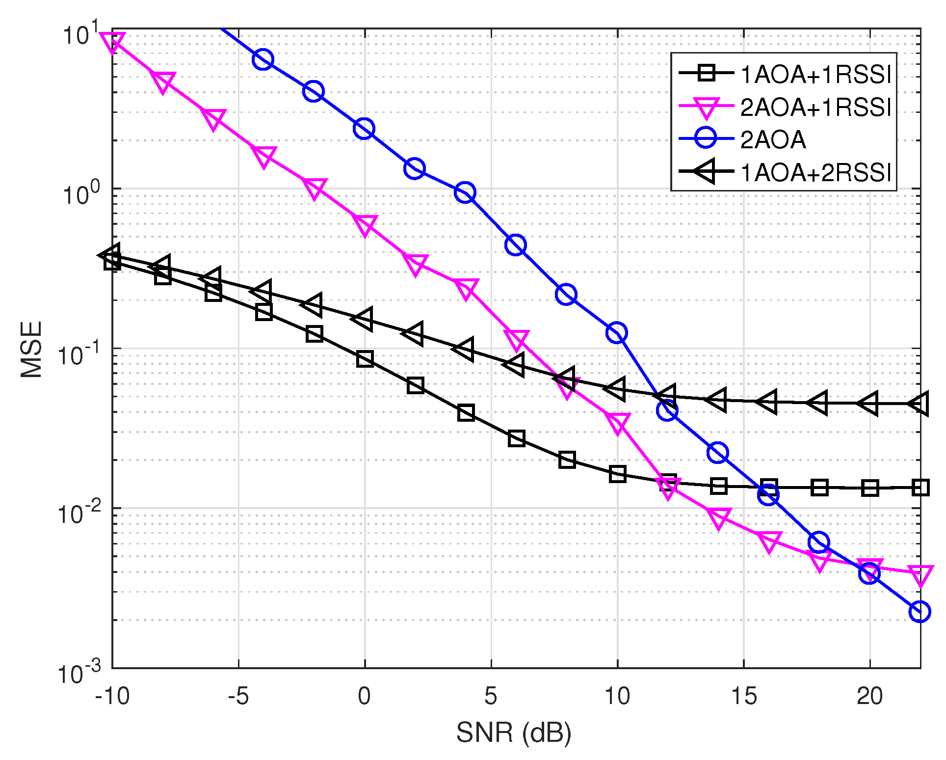
5.1.2. Localization with Correlated Noises
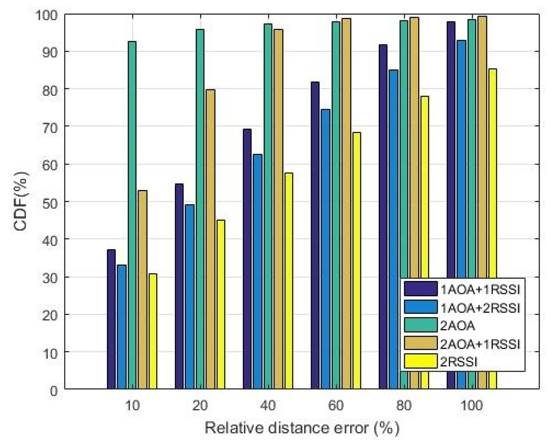
5.2. Accuracy
6. Conclusions
Author Contributions
Funding
Conflicts of Interest
Abbreviations
| AOA | Angle of Arrival |
| FDOA | Frequency Difference of Arrival |
| GPS | Global Positioning System |
| MSE | Mean Square Error |
| MUSIC | Multiple Signal Classification |
| OFDM | Orthogonal Frequency Division Multiplexing |
| PDOA | Power Difference of Arrival |
| RDE | Relative Distance Error |
| RF | Radio Frequency |
| RSSI | Receive Signal Strength Indicator |
| SNR | Signal to Noise Ratio |
| TDOA | Time Difference of Arrival |
| VANET | Vehicular Ad-Hoc Network |
References
- Dargie, W.; Poellabauer, C. Fundamentals of Wireless Sensor Networks: Theory and Practice; Wiley Publishing: West Sussex, UK, 2010. [Google Scholar]
- Xiong, W.; Hu, X.; Wang, B.; Fang, J. Vehicle node localization without GPS in VANET. In Proceedings of the 2014 International Conference on Connected Vehicles and Expo (ICCVE), Vienna, Austria, 3–7 November 2014; pp. 1068–1073. [Google Scholar]
- Nguyen, T.L.N.; Shin, Y. A new approach for positioning based on AOA measurements. In Proceedings of the 2013 International Conference on Computing, Management and Telecommunications (ComManTel), Ho Chi Minh City, Vietnam, 21–24 January 2013; pp. 208–211. [Google Scholar]
- Fascista, A.; Ciccarese, G.; Coluccia, A.; Ricci, G. A localization algorithm based on V2I communications and AOA estimation. IEEE Sign. Process. Lett. 2017, 2017, 126–130. [Google Scholar] [CrossRef]
- Prince, G.B.; Little, T.D.C. A two phase hybrid RSS/AOA algorithm for indoor device localization using visible light. In Proceedings of the IEEE Global Communications Conference (GLOBECOM), Anaheim, CA, USA, 3–7 December 2012; pp. 3347–3352. [Google Scholar]
- He, T.; Huang, C.; Blum, B.M.; Stankovic, J.A.; Abdelzaher, T. Range-Free localization and its impact on large scale sensor networks. ACM Trans. Embed. Comput. Syst. 2005, 4, 877–906. [Google Scholar] [CrossRef]
- Wang, Y.; Wang, X.; Wang, D.; Agrawal, D.P. Range-Free Localization Using Expected Hop Progress in Wireless Sensor Networks. IEEE Trans. Parallel Distrib. Syst. 2009, 20, 1540–1552. [Google Scholar] [CrossRef]
- Liu, J.; Wang, Z.; Yao, M.; Qiu, Z. VN-APIT: Virtual nodes-based range-free APIT localization scheme for WSN. Wirel. Netw. 2016, 22, 867–878. [Google Scholar] [CrossRef]
- Wang, J.Z.; Jin, H. Improvement on APIT localization algorithms for Wireless Sensor Networks. In Proceedings of the nternational Conference on Networks Security, Wireless Communications and Trusted Computing, Wuhan, China, 25–26 April 2009; pp. 719–723. [Google Scholar]
- Kumar, S.; Kislay, K.; Singh, M.K.; Hegde, R.M. A range-free tracking algorithm in Vehicular Ad-Hoc Networks. In Proceedings of the Twentieth National Conference on Communications (NCC), Kanpur, India, 28 February–2 March 2014; pp. 1–6. [Google Scholar]
- Zhang, D.; Xia, F.; Yang, Z.; Yao, L.; Zhao, W. Localization technologies for indoor human tracking. In Proceedings of the 5th International Conference on Future Information Technology, Busan, Korea, 21–23 May 2010; pp. 1–6. [Google Scholar]
- Masashi, S.; Kawazoe, T.; Ohta, Y.; Murata, M. Indoor localization system using RSSI measurement of Wireless Sensor Network based on ZigBee standard. Wirel. Opt. Commun. 2006, 538, 1–6. [Google Scholar]
- Zhu, X.; Feng, Y. RSSI-based Algorithm for Indoor Localization. Commun. Netw. 2013, 5, 37–42. [Google Scholar] [CrossRef]
- Hamdoun, S.; Rachedi, A.; Benslimane, A. Comparative analysis of RSSI-based indoor localization when using multiple antennas in Wireless Sensor Networks. In Proceedings of the International Conference on Selected Topics in Mobile and Wireless Networking (MoWNeT), Montreal, QC, Canada, 19–21 August 2013; pp. 146–151. [Google Scholar]
- Altoaimy, L.; Mahgoub, I.; Rathod, M. Weighted localization in Vehicular Ad Hoc Networks using vehicle-to-vehicle communication. In Proceedings of the Global Information Infrastructure and Networking Symposium (GIIS), Montreal, QC, Canada, 15–19 September 2014; pp. 1–5. [Google Scholar]
- Niculescu, D.; Nath, B. Ad hoc positioning system (APS) using AOA. In Proceedings of the IEEE INFOCOM Annual Joint Conference of the IEEE Computer and Communications Societies, San Francisco, CA, USA, 30 March–3 April 2003; Volume 3, pp. 1734–1743. [Google Scholar]
- Ambassa, J.Y.; Peng, H. RSSI-based Indoor Localization Using RSSI-with-Angle-based Localization Estimation Algorithm. Int. J. Sens. Netw. Data Commun. 2015, 4. [Google Scholar] [CrossRef]
- Ceylan, O.; Taraktas, K.F.; Yagci, H.B. Enhancing RSSI Technologies in Wireless Sensor Networks by Using Different Frequencies. In Proceedings of the International Conference on Broadband, Wireless Computing, Communication and Applications, Fukuoka, Japan, 4–6 November 2010; pp. 369–372. [Google Scholar]
- Fang, X.; Nan, L.; Jiang, Z.; Chen, L. Multi-channel fingerprint localisation algorithm for wireless sensor network in multipath environment. IET Commun. 2017, 11, 2253–2260. [Google Scholar] [CrossRef]
- Frank, V.; Jo, V.; Eric, L.; Ingrid, M.; Piet, D. Automated linear regression tools improve RSSI WSN localization in multipath indoor environment. EURASIP J. Wirel. Commun. Netw. 2011, 2011, 38. [Google Scholar]
- Garip, M.T.; Kim, P.H.; Reiher, P.; Gerla, M. INTERLOC: An interference-aware RSSI-based localization and sybil attack detection mechanism for Vehicular Ad Hoc Networks. In Proceedings of the 14th IEEE Annual Consumer Communications & Networking Conference (CCNC), Las Vegas, NV, USA, 8–11 January 2017; pp. 1–6. [Google Scholar]
- Hussein, A.A.; Rahman, T.A.; Leow, C.Y. Performance Evaluation of Localization Accuracy for a Log-Normal Shadow Fading Wireless Sensor Network under Physical Barrier Attacks. Sensors 2015, 15, 30545–30570. [Google Scholar] [CrossRef]
- Ishii, K.; Sato, N. GPS-Free Host Approaching in Mobile Ad-Hoc Networks. In Proceedings of the Seventh International Conference on Innovative Mobile and Internet Services in Ubiquitous Computing, Taichung, Taiwan, 3–5 July 2013; pp. 108–115. [Google Scholar]
- Jais, I.; Ehkan, P.; Ahmad, R.B.; Ismail, I.; Sabapathy, T.; Jusoh, M. Review of angle of arrival (AOA) estimations through received signal strength indication (RSSI) for wireless sensors network (WSN). In Proceedings of the International Conference on Computer, Communications, and Control Technology (I4CT), Kuching, Malaysia, 21–23 April 2015; pp. 354–359. [Google Scholar]
- Jiang, J.R.; Lin, C.M.; Lin, F.Y.; Huang, S.T. ALRD: AOA localization with RSSI differences of directional antennas for Wireless Sensor Networks. In Proceedings of the International Conference on Information Society (i-Society 2012), London, UK, 25–28 June 2012; pp. 304–309. [Google Scholar]
- Kułakowski, P.; Vales-Alonso, J.; Egea-López, E.; Ludwin, W.; García-Haro, J. Angle-of-Arrival localization based on antenna arrays for Wireless Sensor Networks. Comput. Electr. Eng. 2010, 36, 1181–1186. [Google Scholar] [CrossRef]
- Zhang, X.; Feng, B.; Xu, D. Blind Joint Symbol Detection and DOA Estimation for OFDM System with Antenna Array. Wirel. Pers. Commun. 2008, 46, 371–383. [Google Scholar] [CrossRef]
- Xu, J.; Ma, M.; Law, C.L. AOA cooperative position localization. In Proceedings of the IEEE Global Telecommunications Conference, New Orleans, LO, USA, 30 November–4 December 2008; pp. 1–5. [Google Scholar]
- Tanee, D.; Pratana, K. Performance limit of AOA-based localization using MIMO-OFDM channel state information. EURASIP J. Wirel. Commun. Netw. 2017, 2017, 141. [Google Scholar]
- Park, C.; Park, D.; Park, J.; Lee, Y.; An, Y. Localization Algorithm Design and Implementation to Utilization RSSI and AOA of Zigbee. In Proceedings of the 5th International Conference on Future Information Technology, Busan, Korea, 21–23 May 2010; pp. 1–4. [Google Scholar]
- Chen, T.Y.; Chiu, C.C.; Tu, T.C. Mixing and combining with AOA and TOA for the enhanced accuracy of mobile location. In Proceedings of the 5th European Personal Mobile Communications Conference, Glasgow, UK, 22–25 May 2003; pp. 276–280. [Google Scholar]
- Magnani, A.; Leung, K.K. Self-Organized, Scalable GPS-Free Localization of Wireless Sensors. In Proceedings of the IEEE Wireless Communications and Networking Conference, Kowloon, China, 11–15 March 2007; pp. 3798–3803. [Google Scholar]
- Dai, F.; Liu, Y.; Chen, L. A hybrid localization algorithm for improving accuracy based on RSSI/AOA in wireless network. In Proceedings of the International Conference on Computer Science and Service System, Nanjing, China, 11–13 August 2012; pp. 631–634. [Google Scholar]
- Tomic, S.; Beko, M.; Dinis, R. 3-D Target Localization in Wireless Sensor Networks Using RSS and AOA Measurements. IEEE Trans. Veh. Technol. 2017, 66, 3197–3210. [Google Scholar] [CrossRef]
- Tomic, S.; Beko, M.; Dinis, R.; Montezuma, P. Distributed algorithm for target localization in wireless sensor networks using RSS and AOA measurements. Perv. Mob. Comput. 2017, 37, 63–77. [Google Scholar] [CrossRef]
- Mirza, M.A.; Shakir, M.Z.; Slim-Alouini, M. A GPS-free Passive Acoustic Localization Scheme for Underwater Wireless Sensor Networks. In Proceedings of the IEEE 8th International Conference on Mobile Adhoc and Sensor Systems, Valencia, Spain, 17–22 October 2011; pp. 879–884. [Google Scholar]
- Akcan, H.; Kriakov, V.; Brönnimann, H.; Delis, A. GPS-Free Node Localization in Mobile Wireless Sensor Networks. In Proceedings of the 5th ACM International Workshop on Data Engineering for Wireless and Mobile Access, Chicago, IL, USA, 25 June 2006; pp. 35–42. [Google Scholar]
- Piran, M.J.; Murthy, G.R.; Babu, G.P.; Ahvar, E. Total GPS-free Localization Protocol for Vehicular Ad Hoc and Sensor Networks (VASNET). In Proceedings of the Third International Conference on Computational Intelligence, Modelling & Simulation, Langkawi, Malaysia, 20–22 September 2011; pp. 388–393. [Google Scholar]
- Ravindra, S.; Jagadeesha, S.N. Time Of Arrival Based Localization in Wireless Sensor Networks: A Linear Approach. arXiv 2014, arXiv:1403.6697. [Google Scholar]
- Shen, J.; Molisch, A.F.; Salmi, J. Accurate Passive Location Estimation Using TOA Measurements. IEEE Trans. Wirel. Commun. 2012, 11, 2182–2192. [Google Scholar] [CrossRef]
- Takabayashi, Y.; Matsuzaki, T.; Kameda, H.; Ito, M. Target tracking using TDOA/FDOA measurements in the distributed sensor network. In Proceedings of the SICE Annual Conference, Tokyo, Japan, 20–22 August 2008; pp. 3441–3446. [Google Scholar]
- Ma, W.K.; Vo, B.N.; Singh, S.S.; Baddeley, A. Tracking an unknown time-varying number of speakers using TDOA measurements: A random finite set approach. IEEE Trans. Sign. Process. 2006, 54, 3291–3304. [Google Scholar]
- Ho, K.C.; Lu, X.; Kovavisaruch, L. Source Localization Using TDOA and FDOA Measurements in the Presence of Receiver Location Errors: Analysis and Solution. IEEE Trans. Sign. Process. 2007, 55, 684–696. [Google Scholar] [CrossRef]
- Jung, S.Y.; Hann, S.; Park, C.S. TDOA-based optical wireless indoor localization using LED ceiling lamps. IEEE Trans. Consum. Elect. 2011, 57, 1592–1597. [Google Scholar] [CrossRef]
- Cong, L.; Zhuang, W. Hybrid TDOA/AOA mobile user location for wideband CDMA cellular systems. IEEE Trans. Wirel. Commun. 2002, 1, 439–447. [Google Scholar] [CrossRef]
- Ho, K.C. Bias Reduction for an Explicit Solution of Source Localization Using TDOA. IEEE Trans. Sign. Process. 2012, 60, 2101–2114. [Google Scholar] [CrossRef]
- Bocquet, M.; Loyez, C.; Benlarbi-Delai, A. Using enhanced-TDOA measurement for indoor positioning. IEEE Microw. Wirel. Compon. Lett. 2005, 15, 612–614. [Google Scholar] [CrossRef]
- So, H.C.; Chan, Y.T.; Chan, F.K.W. Closed-Form Formulae for Time-Difference-of-Arrival Estimation. IEEE Trans. Sign. Process. 2008, 56, 2614–2620. [Google Scholar] [CrossRef]
- Hekimian, C.W.; Grant, B.; Liu, X.; Zhang, Z.; Kumar, P. Accurate localization of RFID tags using phase difference. In Proceedings of the IEEE International Conference on RFID (IEEE RFID 2010), Orlando, FL, USA, 14–16 April 2010; pp. 89–96. [Google Scholar]
- Li, J.; Guo, F.; Jiang, W. A Linear-correction Least-squares Approach for Geolocation Using FDOA Measurements Only. Chin. J. Aeronaut. 2012, 25, 709–714. [Google Scholar] [CrossRef]
- Ho, K.C.; Chan, Y.T. Geolocation of a known altitude object from TDOA and FDOA measurements. IEEE Trans. Aerosp. Elect. Syst. 1997, 33, 770–783. [Google Scholar] [CrossRef]
- Sun, M.; Ho, K.C. An Asymptotically Efficient Estimator for TDOA and FDOA Positioning of Multiple Disjoint Sources in the Presence of Sensor Location Uncertainties. IEEE Trans. Sign. Process. 2011, 59, 3434–3440. [Google Scholar]
- Kumar, V.; Arablouei, R.; Jurdak, R.; Kusy, B.; Bergmann, N.W. RSSI-based self-localization with perturbed anchor positions. In Proceedings of the 28th IEEE International Symposium on Personal, Indoor and Mobile Radio Communications (IEEE PIMRC 2017), Montreal, AC, Canada, 8–13 October 2017; pp. 1–6. [Google Scholar]
- Li, X. RSSI-Based Location Estimation with Unknown Pathloss Model. IEEE Trans. Wirel. Commun. 2006, 5, 3626–3633. [Google Scholar] [CrossRef]
- Pormante, L.; Rinaldi, C.; Santic, M.; Tennina, S. Performance analysis of a lightweight RSSI-based localization algorithm for Wireless Sensor Networks. In Proceedings of the International Symposium on Signals, Circuits and Systems ISSCS2013, Iasi, Romania, 11–12 July 2013; pp. 1–4. [Google Scholar]
- Guoqiang, M.; Anderson, B.D.O.; Fidan, B. Path loss exponent estimation for Wireless Sensor Network localization. Comput. Netw. 2007, 51, 2467–2483. [Google Scholar]
- Yaghoubi, F.; Abbasfar, A.A.; Maham, B. Energy-Efficient RSSI-Based Localization for Wireless Sensor Networks. IEEE Commun. Lett. 2014, 18, 973–976. [Google Scholar] [CrossRef]
- Zheng, J.; Wu, C.; Chu, H.; Xu, Y. An Improved RSSI Measurement In Wireless Sensor Networks. Proc. Eng. 2011, 15, 876–880. [Google Scholar] [CrossRef]
- Wang, H.; Wan, J.; Liu, R. A novel ranging method based on RSSI. Energy Procedia 2011, 12, 230–235. [Google Scholar] [CrossRef]
- Akcan, H.; Evrendilek, E. GPS-free directional localization via dual wireless radios. Comput. Commun. 2012, 35, 1151–1163. [Google Scholar] [CrossRef]
- Sahu, P.K.; Wu, E.H.K.; Sahoo, J. DuRT: Dual RSSI Trend Based Localization for Wireless Sensor Networks. IEEE Sens. J. 2013, 13, 3115–3123. [Google Scholar] [CrossRef]
- Shi, H. A new weighted centroid localization algorithm based on RSSI. In Proceedings of the IEEE International Conference on Information and Automation (ICIA), Shenyang, China, 6–8 June 2012; pp. 137–141. [Google Scholar]
- Mukhopadhyay, B.; Sarangi, S.; Kar, S. Performance evaluation of localization techniques in Wireless Sensor Networks using RSSI and LQI. In Proceedings of the Twenty First National Conference on Communications (NCC), Mumbai, India, 27 February–1 March 2015; pp. 1–6. [Google Scholar]
- Stoica, P.; Nehorai, A. Music, maximum likelihood, and cramer-rao bound. IEEE Trans. Acoust. Speech Sign. Process. 1989, 37, 720–741. [Google Scholar] [CrossRef]
- Fascista, A.; Ciccarese, G.; Coluccia, A.; Ricci, G. Angle of arrival-based cooperative positioning for smart vehicles. IEEE Trans. Intell. Transp. Syst. 2017, 99, 1–13. [Google Scholar] [CrossRef]
- Boushaba, M.; Hafid, A.; Benslimane, A. High accuracy localization method using AOA in sensor networks. Comput. Netw. 2009, 53, 3076–3088. [Google Scholar] [CrossRef]
- Robertson, A.; Kompella, S.; Molnar, J.; Fu, M.D.F.; Perkins, D. Distributed Transmitter Localization by Power Difference of Arrival (PDOA) on a Network of GNU Radio Sensors; Technical Report; Naval Research Laboratory: Washington DC, USA, 2015. [Google Scholar]
- Guo, S.; Jackson, B.; Wang, S.; Inkol, R.; Arnold, W. A novel density-based geolocation algorithm for a noncooperative radio emitter using power difference of arrival. In Proceedings of the Wireless Sensing, Localization, and Processing VI, Orlando, FL, USA, 24 May 2011. [Google Scholar]
- Frank, B.G. Smart Antennas with MATLAB; McGraw-Hill Education: New York, NY, USA, 2015. [Google Scholar]
- Tran, L.C.; Wysocki, T.A.; Mertins, A.; Seberry, J. A generalized algorithm for the generation of correlated rayleigh fading envelopes in radio channels. In Proceedings of the 19th IEEE International Parallel and Distributed Processing Symposium, Denver, CO, USA, 4–8 April 2005; p. 238.2. [Google Scholar]
- Tran, L.C.; Wysocki, T.A.; Mertins, A.; Seberry, J. A generalized algorithm for the generation of correlated rayleigh fading envelopes in wireless channels. EURASIP J. Wirel. Commun. Netw. 2005, 2005, 710469. [Google Scholar] [CrossRef]
- Le, N.P.; Tran, L.C.; Safaei, F. Energy-efficiency analysis of per-subcarrier antenna selection with peak-power reduction in MIMO-OFDM wireless systems. Int. J. Antennas Propag. 2014, 2014, 313195. [Google Scholar] [CrossRef]
- Tran, L.C.; Mertins, A.; Wysocki, T.A. Quasi-orthogonal space-time-frequency codes in MB-OFDM UWB. Comput. Electr. Eng. 2010, 36, 766–774. [Google Scholar] [CrossRef]
- Tran, L.C.; Wysocki, T.A.; Mertins, A.; Seberry, J.; Mertins, A.; Spence, S.A. Novel constructions of improved square complex orthogonal designs for eight transmit antennas. IEEE Trans. Inform. Theory 2009, 55, 4439–4448. [Google Scholar] [CrossRef]
- Tran, L.C.; Mertins, A.; Wysocki, T.A. Unitary differential space-time-frequency codes for MB-OFDM UWB wireless communications. IEEE Trans. Wirel. Commun. 2013, 12, 862–876. [Google Scholar] [CrossRef]


| Method | Bearing Measurement | Advantages | Disadvantages | Literature |
|---|---|---|---|---|
| Time of Arrival (TOA) | Distance | Simple to calculate | Require strict synchronization | [36,37,38,39,40] |
| Time of Arrival (TOA) | Distance | Simple to calculate | Require strict synchronization | [36,37,38,39,40] |
| Time Difference of Arrival (TDOA) | Distance | Asynchronous process | Time delay can be large and require large bandwidth | [41,42,43,44,45,46,47,48] |
| Frequency Difference of Arrival (FDOA) (i.e., Differential Doppler) | Distance | Robust for moving nodes | Hard to merely use FDOA to locate nodes because of its non-linear equation. FDOA is normally combined with TDOA | [43,44,49,50,51,52] |
| Received Signal Strength Indicator (RSSI) | Distance | Simplest method and do not require complicated hardware | Need preliminary knowledge on the propagation environment and subjective to noise | [12,13,14,15,23,53,54,55,56,57,58,59,60,61,62,63] |
| Angle of Arrival (AOA) | Angle | Robust to noise | More complex and expensive than other types | [3,4,5,16,26,28,29,64,65,66] |
| Power Difference of Arrival (PDOA) | Distance | Do not need many anchors in the network | Affected by shadowing and noise effects | [67,68] |
| Number of Anchors | Method | Measurements | Mathematical Formulas | Graphical Representation |
|---|---|---|---|---|
| 1 | 1AOA + 1RSSI | , |  | |
| 2 | 2AOA |  | ||
| 2 | 2RSSI |  | ||
| 2 | 1AOA + 2RSSI | , , |  | |
| 2 | 2AOA + 1RSSI | , , |  | |
| 2 | 2AOA + 2RSSI | , |  | |
| 3 | 3RSSI | , |  | |
| 3 | Weighted 3RSSI | , |  |
© 2019 by the authors. Licensee MDPI, Basel, Switzerland. This article is an open access article distributed under the terms and conditions of the Creative Commons Attribution (CC BY) license (http://creativecommons.org/licenses/by/4.0/).
Share and Cite
Nguyen, N.M.; Tran, L.C.; Safaei, F.; Phung, S.L.; Vial, P.; Huynh, N.; Cox, A.; Harada, T.; Barthelemy, J. Performance Evaluation of Non-GPS Based Localization Techniques under Shadowing Effects. Sensors 2019, 19, 2633. https://doi.org/10.3390/s19112633
Nguyen NM, Tran LC, Safaei F, Phung SL, Vial P, Huynh N, Cox A, Harada T, Barthelemy J. Performance Evaluation of Non-GPS Based Localization Techniques under Shadowing Effects. Sensors. 2019; 19(11):2633. https://doi.org/10.3390/s19112633
Chicago/Turabian StyleNguyen, Ngoc Mai, Le Chung Tran, Farzad Safaei, Son Lam Phung, Peter Vial, Nam Huynh, Anne Cox, Theresa Harada, and Johan Barthelemy. 2019. "Performance Evaluation of Non-GPS Based Localization Techniques under Shadowing Effects" Sensors 19, no. 11: 2633. https://doi.org/10.3390/s19112633
APA StyleNguyen, N. M., Tran, L. C., Safaei, F., Phung, S. L., Vial, P., Huynh, N., Cox, A., Harada, T., & Barthelemy, J. (2019). Performance Evaluation of Non-GPS Based Localization Techniques under Shadowing Effects. Sensors, 19(11), 2633. https://doi.org/10.3390/s19112633