Dynamics of Lingulodinium polyedra Development in the Bulgarian Part of Black Sea (1992–2022)

Abstract

Long-term data on the phytoplankton of the Bulgarian Black Sea (BBS) coast describe three states for the ecosystem: a “pristine” reference phase (1954–1970 years); an intensive anthropogenic eutrophication (1970–1992 years) phase; and a post-eutrophication phase after the early 1990s of the 20th century. The eutrophication period is characterised by ecosystem degradation and intense phytoplankton blooms, some of which were formed by the potentially toxic species Lingulodinium polyedra. This warm-water species is a red tide former that is associated with fish and shellfish mortality events. In the 1980s, L. polyedra reached the highest biomass of 84.4 g·m⁻³ in Varna Bay, BBS. The aim of this study (1992–2022) was to provide an overview of the development of L. polyedra in the phytoplankton biocenosis in the Bulgarian part of the Black Sea, taking into account the influence of anthropogenic stress and the climatic variables NAO and SST on the development of the species population. An analysis of the distribution of the dinoflagellate L. polyedra is based on a total of 5126 phytoplankton samples collected during the period between 1992 and 2022 under projects led by the Institute of Fish Resources, Varna. The samples were analyzed using standard methods validated for the Black Sea, and phytoplankton abundance and biomass were determined. The species are most abundant in summer in the coastal marine areas exposed to anthropogenic influence. During the analyzed period, a decrease in the abundance and biomass of L. polyedra in Bulgarian Black Sea waters were observed. It was found that the influence of climatic factors such as NAO and SST on the species population is from weak to moderate, and the correlation with NAO cycles is better expressed.

1. Introduction

1.1. Taxonomy of Lingulodinium polyedra

The marine dinoflagellate Lingulodinium polyedra (F.Stein) J.D.Dodge 1989 (synonyms: Lingulodinium polyedrum; Gonyaulax polyedra F.Stein, 1883; Hystrichosphaeridium machaerophorum Deflandre and Cookson, 1955; Lingulodinium machaerophorum (Deflandre and Cookson) Wall, 1967) [1], Lingulaulax polyedra (F.Stein) M.J.Head, K.N.Mertens and R.A.Fensome 2024 [1] is a common phytoplanktonic species in the Bulgarian Black Sea waters [2,3]. In the present study, we used the old name of the species to ensure comparability with publications written over the past 20 years. In our opinion, the new name has not yet been sufficiently established (as it was only changed in 2024).

According to Guiry and Guiry (2024) [1], the taxonomic classification of the species is: Chromista (Kingdom)—Harosa (Subkingdom)—Alveolata (Infrakingdom)—Myzozoa (Phylum)—Dinozoa (Subphylum)—Dinoflagellata (Infraphylum)—Dinophyceae (Class)—Gonyaulacales (Order)—Gonyaulacaceae (Family)—Lingulodinium (Genus)—Lingulodinium polyedra (Species).

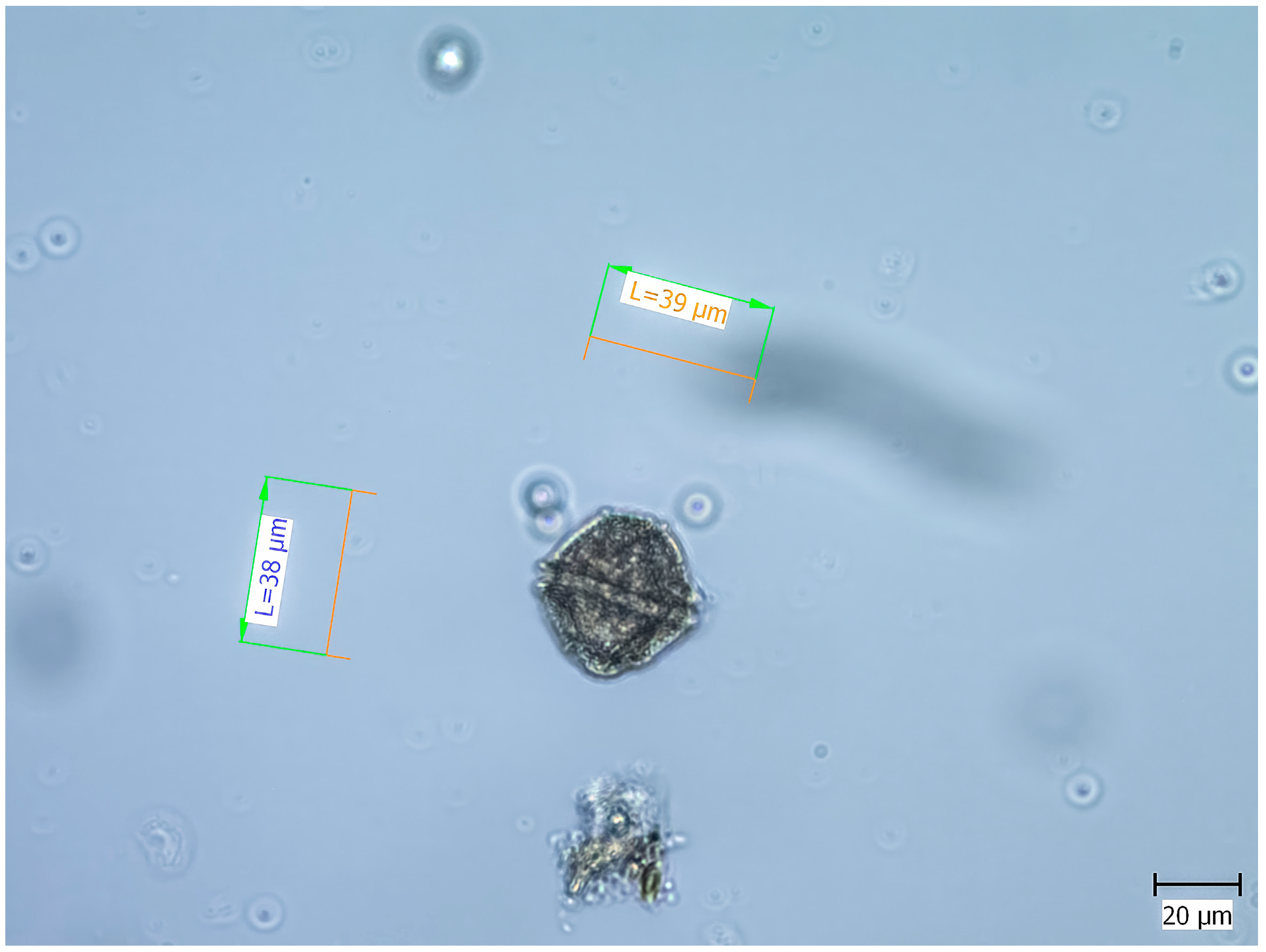
1.2. Morphology of L. polyedra

L. polyedra “is an armoured, marine dinoflagellate species, with dark, orange-brown chloroplasts” [4] (p. 45).

The dimensions of the cells of L. polyedra are “angular, roughly pentagonal and polyhedral-shaped, 40–54 µm in length and 37–53 µm in transdiameter width. No apical horn or antapical spines present. Thecal plates are thick, well defined, and coarsely areolate. Distinct ridges are present along the plate sutures. Numerous large trichocyst pores are present within areolae” [4] (p. 45).

The species found in the Black Sea do not differ from the morphology described above.

1.3. Ecology of L. polyedra

L. polyedra is a bioluminescent planktonic species commonly found in neritic waters [5,6]. “It is responsible for magnificent displays of phosphorescence at night in warm coastal waters” [4] (p. 45).

The feeding of L. polyedra is mixotrophic [7]. L. polyedra “reproduces asexually by binary fission. Sexual reproduction is also part of the life cycle of this species producing spherical spiny cysts” [4] (p. 46).

“Often, the final phase or step of a red tide (of L. polyedra) is the formation of cysts, which act as a resistant resting stage that remains in sediments until conditions are again favorable for growth” [8,9] (p. 2).

The warm-water species Lingulodinium polyedra “is a red tide former that has been associated with fish and shellfish mortality events” [4] (p. 45).

The species is included in the taxonomic reference list of harmful microalgae [10].

1.4. Harmful Algal Blooms (HABs) of L. polyedra Around the World

High concentrations of phytoplankton blooms lead to a change in the colour of sea water and depletion of oxygen in the bottom layers, which causes the demise of fish and other benthos.

During the bloom of L. polyedra, (abundance 700 mln. cells·m⁻³) in Serubal Bay, Portugal, the sea water was reported to have changed to a brown colour [11]. In Todos Santos Bay (Pacific coast of Mexico), the species was recorded in bloom with an abundance ranging from 100 to 1000 mln. cells·m⁻³ [11].

In the period 2000–2015, in Acapulco Bay, Guerrero, Mexico, a bloom of the species was recorded as reaching 286 mln. cells·m⁻³ [12].

In 2021, on the French Atlantic coast, the abundance of the species was reported to be up to 3600 mln. cells·m⁻³ [13].

1.5. Distribution and Blooms of L. polyedra in the Black Sea

The species was first described in the Black Sea by Zernov [14].

In October 1909, S.A. Zernov observed the appearance of rusty-red stripes (bloom) caused by L. polyedra in the coastal zone of Sevastopol [15].

L. polyedra is a mass phytoplanktonic species for the Black Sea, one of the most common in the coastal waters [16,17]. It is usually found in spring and summer [18].

The higher abundances of L. polyedra in the Bulgarian Black Sea waters are related to the influence of the eutrophication processes taking place here over the years [19].

It was found that “Regardless of the temperature variations in the Black Sea or maybe as a result of them, the long-term data models show three states of the ecosystem of the Black Sea North West Shelf (BSNWS) [20]. They include:

• A low-productive ecosystem before 1970 or the so-called “pristine” reference phase
• A highly productive eutrophic system during the 1980s or a phase of intensive anthropogenic eutrophication and destruction of the Black Sea ecosystem
• A transitional, relatively low productive system after the beginning of the 1990s or the so-called post-eutrophication phase in the development of the Black Sea ecosystem” [21] (p. 2).

For the first time in Bulgarian Black Sea waters, the dinflagellate L. polyedra was recorded in the 1950s by Vyara Petrova (IFR-Varna [22]. The species was found in a vast sea area from the village of Kranevo to Cape Maslen. The minimum salinity at which it developed was 12‰. It was also recorded in the brackish Varna Lake [22].

In the pre-eutrophication period, L. polyedra was recorded as a common phytoplankton species in Bulgarian marine waters, but not as a causative agent of blooms [2,3,23,24].

In the autumn of 1956, it was recorded in the biomass of the dominant phytoplanktonic species in the southern coastal waters off the town of Michurin [25].

During most of the eutrophication period (1970 to early 1990s), L. polyedra continued to dominate in the phytoplankton biomass, but monospecific blooms were not recorded [16,26]. The species was found to accompany the formation of “red tides” by Prorocentrum cordatum (Ost.) Dodge, 1976. In the 1970s and 1980s, phytoplankton blooms were a serious environmental problem in the Bulgarian Black Sea waters [27,28,29,30,31,32].

At the end of the eutrophication period in several consecutive years (from 1987 to 1992) in the anthropogenically loaded waters of Varna Bay [21] blooms of L. polyedra were recorded. The abundance of the species exceeded the limit for a bloom (1000 mln. cells·m⁻³), and due to the large cell sizes (40–54 µm in length [4]), it produced a phytoplanktonic biomass above 30,000 mg·m⁻³—a “red tide” level above which degradation of the marine ecosystem begins [19].

Such blooms were observed during the warm months of the year: 1987—an abundance of 1600.00 mln. cells·m⁻³ and biomass 84,403.20 mg·m⁻³ (September, Varna Bay), 1988—an abundance of 1200.00 mln. cells·m⁻³ and biomass 63,302.40 mg·m⁻³ (August, Varna Bay), 1989—an abundance of 1200.00 mln. cells·m⁻³ and biomass 63,302.40 mg·m⁻³ (August, Varna Bay) and 1992—an abundance of 1000.00 mln. cells·m⁻³ and biomass 52,752.00 mg·m⁻³ (August, Varna Bay) [19,33].

Moncheva [33] notes that it is possible that a bloom of L. polyedra was formed as early as November 1984 because, in the same year, cysts of the species were found in bottom sediments. The author assumes that the cyst formation of L. polyedra is associated with mass development to a state of bloom [33].

Moncheva [16] has found that the strain of L. polyedra found along the Bulgarian coast develops optimally at a water temperature of 22.8 °C and a salinity of 17.07‰.

During the post-eutrophication period, L. polyedra was periodically involved in the formation of phytoplanktonic biomass in the northwestern shelf of the Black Sea (from September to October) [34]. In September 2005, the species was registered in Bulgarian waters with a maximum abundance of 8.32 mln. cells·m⁻³ [17]. In August 2008, the species was observed in the Romanian coastal waters with a maximum biomass of 1200 mg·m⁻³ [35].

Although, in recent decades, many scientific publications on the Black Sea have reported a tendency for a decrease in the concentration of nutrients [20,21,32,36,37,38,39,40]. In October 2020 (in Odessa Bay, the Northwestern part of the Black Sea), the development of the dinoflagellate L. polyedra was registered with an abundance of 56,100 mln. cells·m⁻³. “The red tide was so huge and dense that the water glowed at night due to the bioluminescence characteristic of this species“ [15] (p. 1).

1.6. Toxins Produced by L. polyedra

According to data in the literature, L. polyedra is associated with the production of two types of toxic substances—saxitoxin and yessotoxins (YTXs).

In the early 1990s, Bruno et al. [41] reported “the presence of a paralytic shellfish poison (PSP) toxin, saxitoxin, in water samples taken during a bloom of” L. polyedra [4] (p. 46). “In the case of serious intoxication, PSP leads to a variety of neurological symptoms culminating in respiratory arrest and cardiovascular shock or death” [42] (p. 353).

L. polyedra, “the major dinoflagellate species in the recent algal blooms in southern California in 2011 and 2013, was shown to induce allergic responses in humans exposed to the bloom. The chemical natures of the compounds produced by L. polyedrum which induce this response are as of yet unknown” [43] (p. 1).

In studies published in recent years, the toxins associated with L. polyedra are yessotoxins [13,44,45,46,47,48,49]. Huang et al. [49] (p. 2) found that “currently, several dinoflagellates including Protoceratium reticulatum, Lingulaulax polyedra (=Lingulodinium polyedra) and a few Gonyaulax species are known to produce YTXs”. Paz et al. [44] and Pistocchi et al. [48] found yessotoxins in a monoculture of L. polyedra. Pistocchi et al. [48] established that “toxic and non-toxic strains were also reported from different areas [44,47]” [48] (p. 146). The results evidence a high variability in the toxicity of this species or, alternatively, that L. polyedrum becomes toxic only under certain environmental conditions [48].

With regard to the Adriatic area Granéli and Tuner [50] confirmed that, “from 1976 to 1984, this species sustained severe blooms causing seawater discolorations, although these events were never associated with toxic mussels” [48] (p. 147).

Meave del Castillo and Zamudio-Resendiz [12] determined that concentrations of L. polyedra higher than one mln. cells·m⁻³ are a prerequisite for the development of a harmful bloom and for the manifestation of the toxicity of the species.

YTXs are found in shellfish from Europe, Asia, and North America. No cases of yessotoxins poisonings in humans have been reported, but in animals, YTXs have been found to exhibit strong toxic properties [46].

Although, in 2021, a strong bloom of L. polyedra (3600 mln. cells·m⁻³) was found along the French coast, “concentrations of yessotoxins up to 747 μg/kg were recorded in mussels, below the safety threshold of 3750 μg/kg. Oysters, clams and cockles also were contaminated with yessotoxins, but at lower concentrations. The established cultures did not produce yessotoxins at detectable levels, although yessotoxins were detected in the sediment.” [13] (p. 1).

In recent years, yessotoxins have been recorded in the Novorossiysk Bay [51], the Caucasus coast [52] and in Bulgarian Black Sea waters [17]. With an abundance of L. polyedra of 0.3 mln. cells·m⁻³, in Black Sea waters, YTXs have been found in low concentrations in mussel tissues [17,52].

It was established for the Bulgarian marine waters that “despite the variety of potentially toxic species no human health problems have been recorded but it isn’t clear if it is due to misdiagnosis or the strains present in the area are non-toxic or weakly toxic due to lack of proper investigations” [17] (p. 327).

It was concluded that in the Bulgarian part of the Black Sea, “potentially toxic species reach ten times higher abundance“ [17] (p. 327) compared to other areas of the sea, and the abundance of L. polyedra is 28 times higher [17]. “Suggesting a potential threat of toxic event does exist” [17] (p. 327).

The aim of this study (1992–2022) was to provide an overview of the development of L. polyedra in the phytoplankton biocenosis in the Bulgarian part of the Black Sea, taking into account the influence of anthropogenic stress and the climatic variables NAO and SST on the development of the species population.

2. Materials and Methods

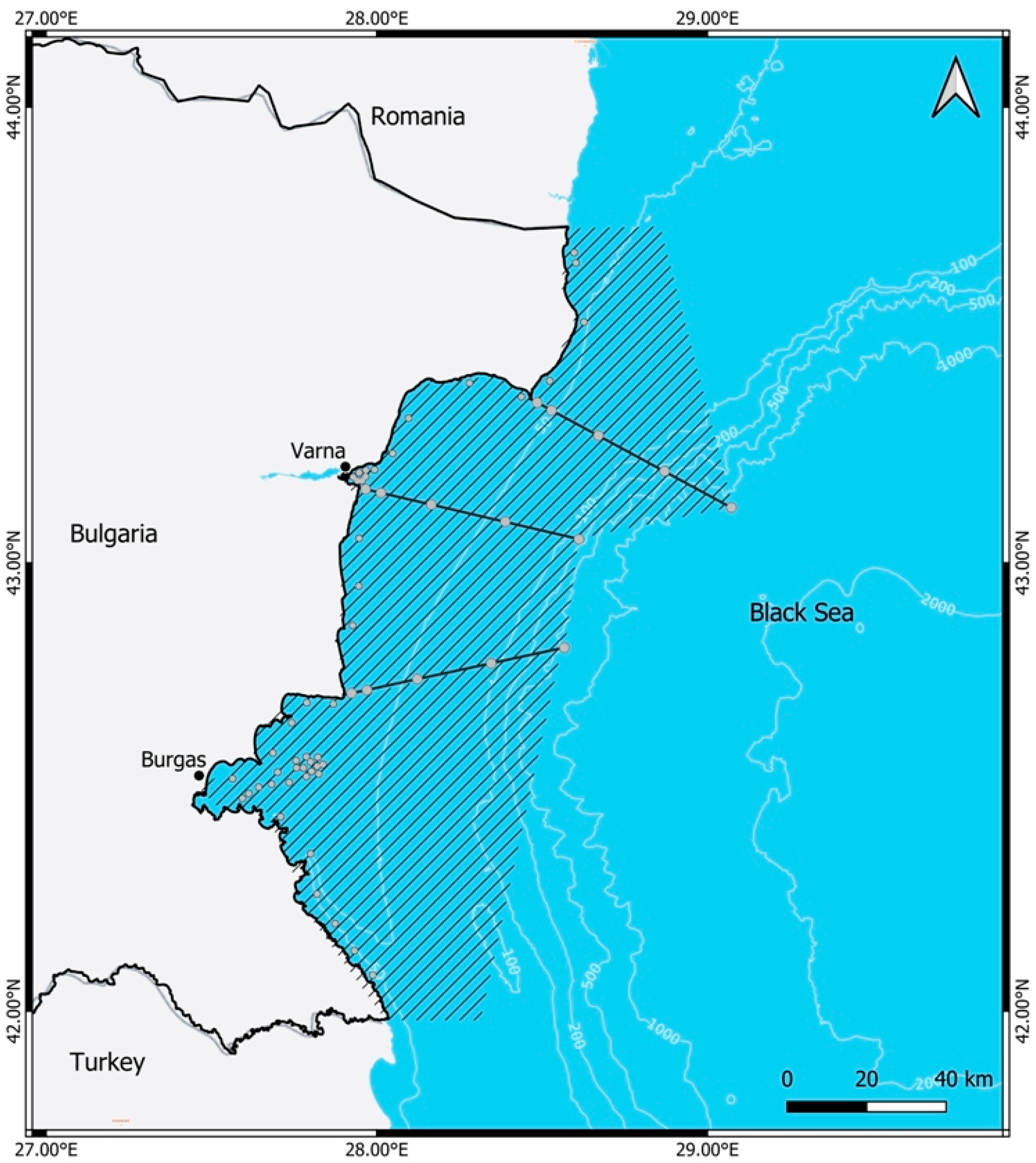
2.1. Study Area

During various research programmes and projects, in the period 1992–2022, the Bulgarian Black Sea water area stretching from Cape Sivriburun in the North to the Rezovska River in the South and with a distance from the Bulgarian coast up to 30 nautical miles was studied (Figure 1). In the study area, from North to South, the 3 main profiles in the monitoring scheme of IFR-Varna are shown—off Cape Kaliakra, Cape Galata and Cape Emine with location of the stations at 1, 3, 10, 20 and 30 nautical miles (used qGIS 3.34.9 Prizren with data sources) [53,54].

2.2. Field Sampling

During the research period (1992–2022) a total of 5126 phytoplankton samples were collected in Bulgarian Black Sea waters monthly and seasonally each year.

The sampling was conducted at 316 stations (as part of national and international monitoring programs of the Institute of Fish Resources (IFR)—Varna, Bulgaria with Niskin bottles, Hydro-Bios, Kiel, Germany (5 L) at the standard depths (0, 5, 10, 25, 50, 75, 100 m). The phytoplankton samples (500 mL) were fixed with 37% formaldehyde solution at a final concentration of 2% on board the research vessels (RV).

2.3. Sample Handling in the Laboratory

The seawater samples were transported to the hydrobiological laboratory (IFR-Varna) and were concentrated by the settling method [55].

The qualitative (taxonomic structure) and quantitative (abundance, biomass) analyses of the samples were performed with a conventional light microscope (Reichert Carl ZEISS, Carl Zeiss GmbH, Wien, Austria; Nikon Eclipse 400, Nikon Instruments, Melville, USA and OlympusBX41, Olympus, Tokyo, Japan), (with magnification 100×, 200×, and 400×) in counting chambers of Palmer–Maloney—0.05 mL and Sedgwick Rafter—1 mL, using standard protocols for the Black Sea [56].

The cell volume of phytoplankton was calculated using geometric formulas [57,58]. The wet biomass was assumed to be equal to the cell volume (r = 1). The biomass was determined through morphometric measurement of phytoplankton units [57].

During the period of this study (1992–2022), the qualitative and quantitative analysis of phytoplankton samples was carried out by various researchers from the Institute of Fish Resources in Varna (Agricultural Academy—Sofia, Bulgaria): Dr. Detelina Murdjeva (1992), Dr. Violeta Velikova (1992–2003), Prof. Dr. Daniela Klisarova (since 1995 to the present day) and Dr. Dimitar Gerdzhikov (since 2002 to the present day).

Taxonomic reference books on the phytoplankton of the Black Sea and the World’s Oceans have been used in the taxonomic determination of the dinoflagellate L. polyedra [1,4,6,59]. In support of the taxonomic identification of the species, original microphotographs from the Black Sea were used. One of them is presented in Figure 2.

Frequency of occurrence (%) was determined by dividing the number of phytoplankton samples in which the species was found by the total number of samples for a given time period and multiplying the result by 100 [60].

The information on the maximum concentrations of L. polyedra for the period 1987–1992 is based on literary sources and our own research [19,33].

2.4. Climate Data

The monthly data for air temperature measured at the meteorological stations Varna and Burgas in the period 1992–2022 are used for the research. The air temperature data are published in the meteorological annuals and bulletins of the National Institute of Meteorology and Hydrology (NIMH), Bulgaria. To clarify the climate impact on the frequency and abundance of L. polyedra the December to March North Atlantic Oscillation Indices (NAOI)—Hurrel station dataset [61,62] were used.

The sea surface temperature (SST) data, version v2.1, were obtained from the Integrated Climate Data Center in Hamburg, Germany, covering the period from September 1981 to the present. These data, known as the OISST dataset (formerly Reynolds SST), were generated using the optimum interpolation (OI) technique, combining Advanced Very High-Resolution Radiometer (AVHRR) infrared channels with buoy and ship observations. These data are provided on a 0.25° spatial grid. For analysis of the Bulgarian Black Sea coast, monthly mean SST data were used, with bilinear interpolation applied to estimate values outside the grid mesh. In order to evaluate the impact of SST on the frequency and abundance of L. polyedra the average values from the following regions: Duranulak, Shabla, Varna, and Tsarevo were taken (

Table 1. The geographical location of the points for SST.

	Longitude (Eastern)	Latitude (Northern)
Durankulak	28.9539	43.6849
Shabla	28.9799	43.5333
Varna	28.3017	43.2026
Tsarevo	28.2239	42.1703

).

2.5. Studying the Dependence of L. polyedra on Sea Surface Temperature (SST) and North Atlantic Oscillation Indices (NAOI)

The development of the species L. polyedra over the years in the BBS waters was analysed using Multivariate analysis of variance (MANOVA) with Post Hoc Tukey test, Bivariate correlation and Nonlinear regression analysis.

The aim was to compile nonlinear predictive models defining the effect of SST and NAO on the changes of the L. polyedra abundance, biomass, volume of cells and frequency of occurrence in the Bulgarian Black Sea waters. Level of significance p < 0.05 were considered statistically significant. Levene’s test of equality of error variances was used to examine the homogeneity of the samples. Predictive models were established by the Cubic equation:

$$Y=\mathit{const}.+b_{1}x+b_2{x}^2+b_3{x}^3$$

(1)

where $Y$ is the observed parameter (abundance, biomass, volume of cells and frequency of occurrence of L. polyedra), $x$ is the fixed factor (SST or NAO), and $\mathit{const}.;b_1;b_2;b_3$ are the model coefficients.

To analyze the development of the species L. polyedra over the years, the population dynamics were examined for separate shorter periods. The following abbreviations were used:

D1—First decade 1992–2000; D1F1—First five-year period of the first decade 1992–1995; D1F2—Second five-year period of the first decade 1996–2000;

D2—Second decade 2001–2010; D2F1—First five-year period of the second decade 2001–2005; D2F2—Second five-year period of the second decade 2006–2010;

D3—Third decade 2011–2020; D3F1—First five-year period of the third decade 2011–2015; D3F2—Second five-year period of the third decade 2016–2020;

D4—Fourth decade 2021–2022; D4F1—First five-year period of the fourth decade 2021–2022.

The basic statistics for the fourth decade are calculated but are not taken into account in the analysis of the results, since this period covers only the last two years of the studied period.

Specialized software for phytoplankton analyses Phytomar 2.0 [63], SPSS Statistics 26.0, and Excel (Microsoft Office, Redmond, Washington DC, USA) were used for data calculations and graphs.

3. Results

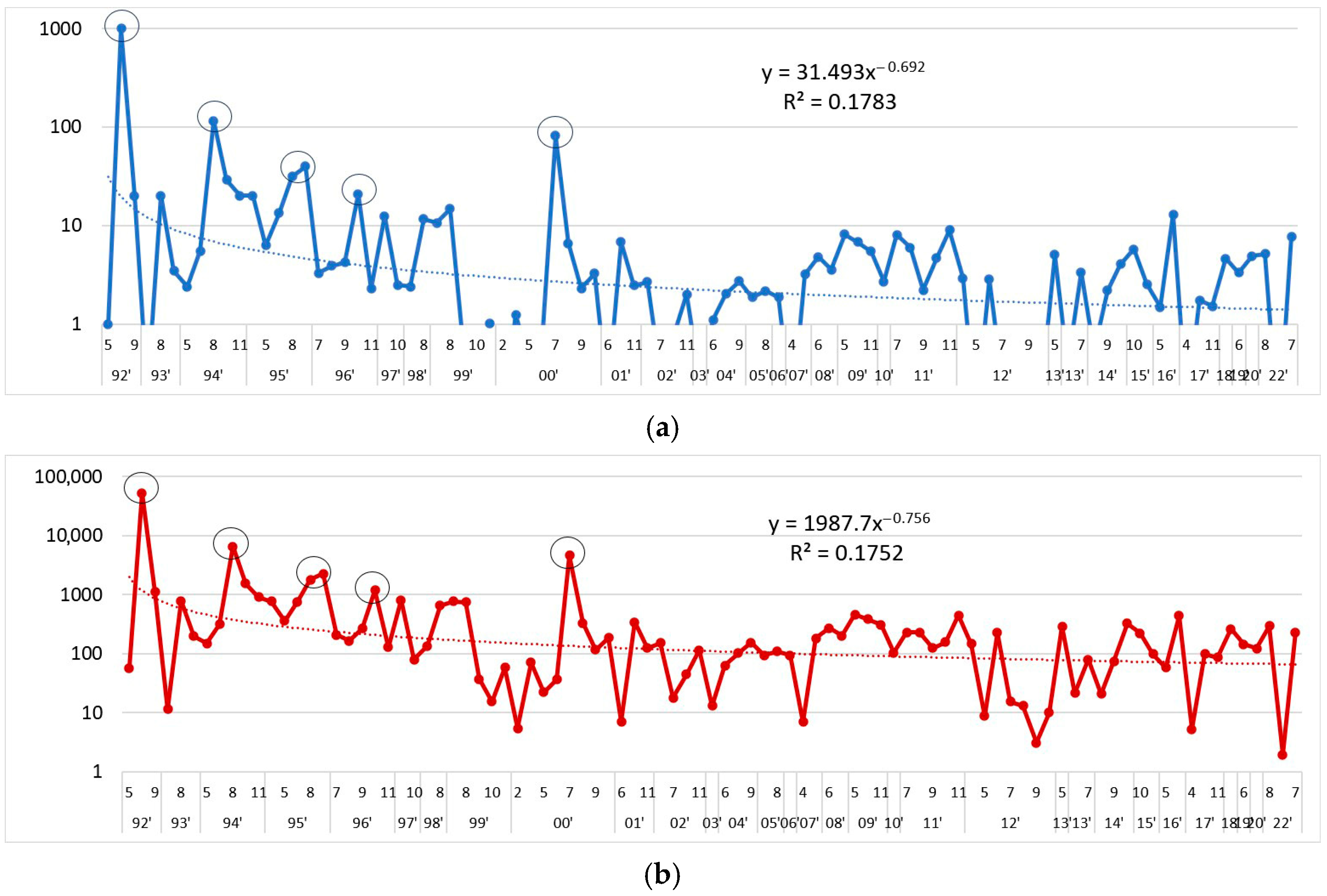
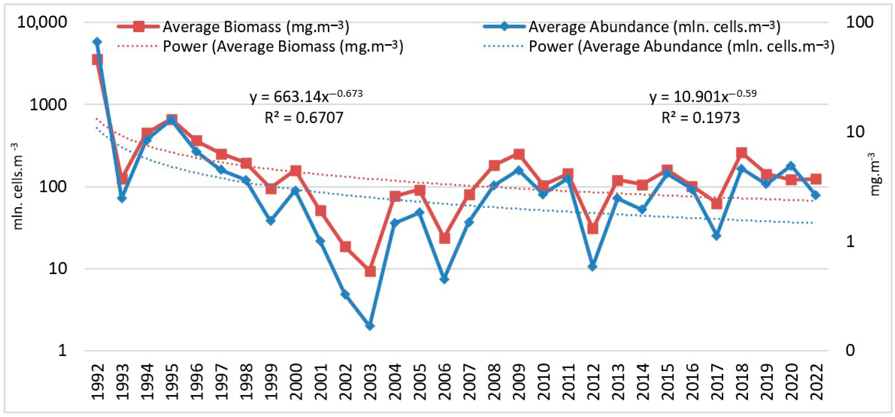
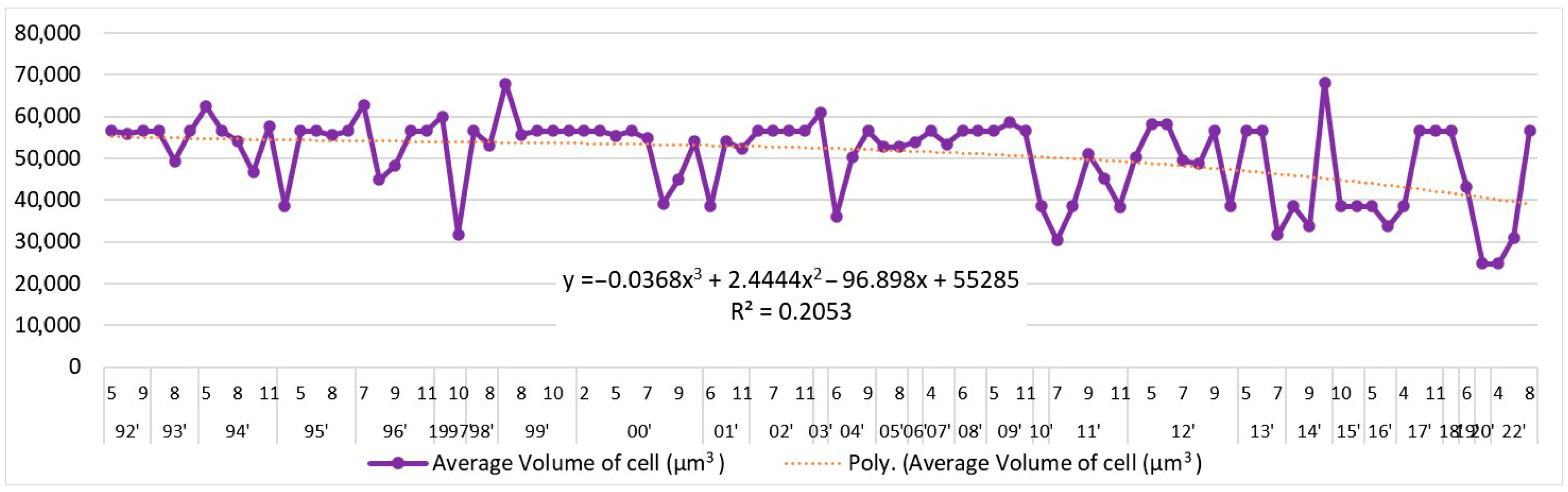
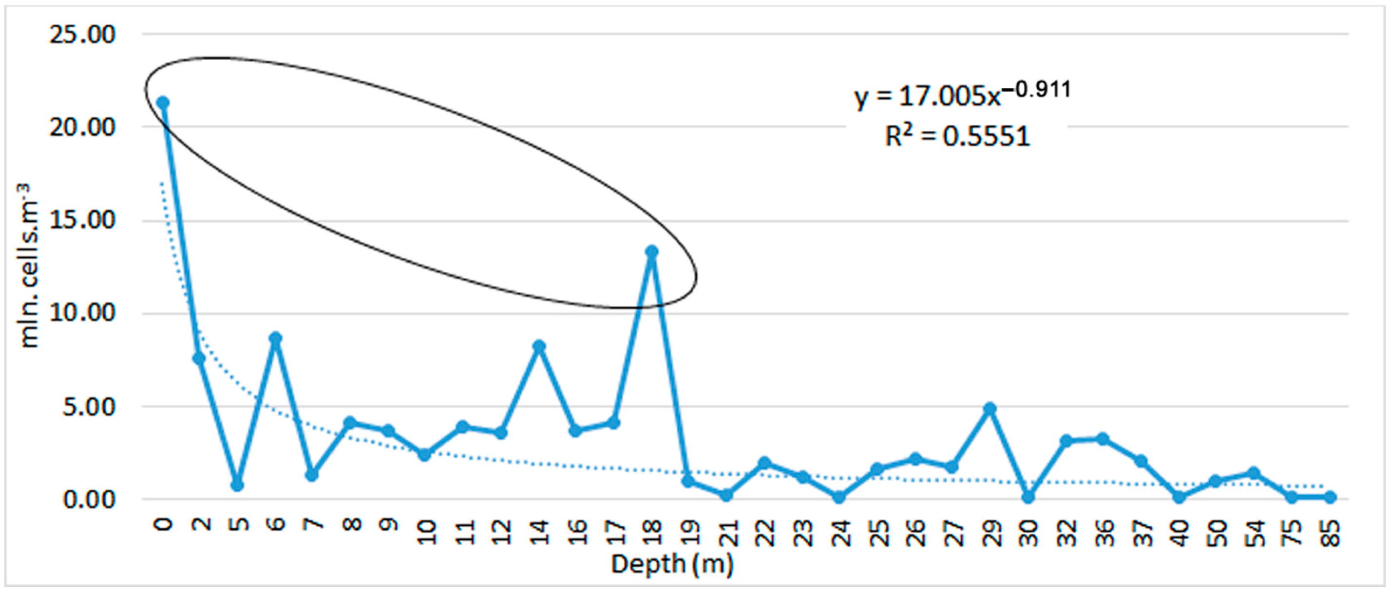
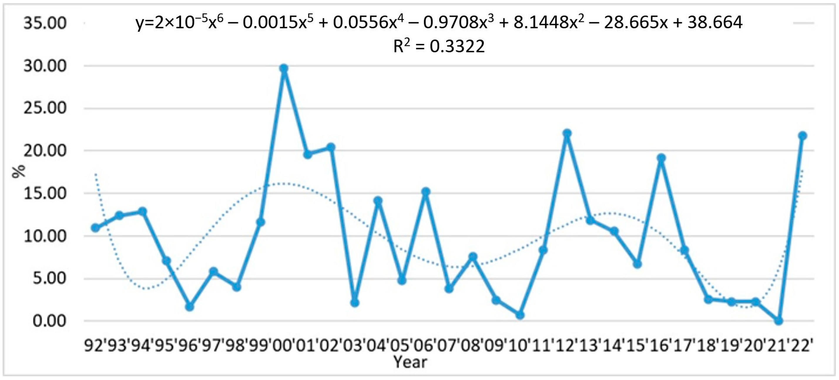
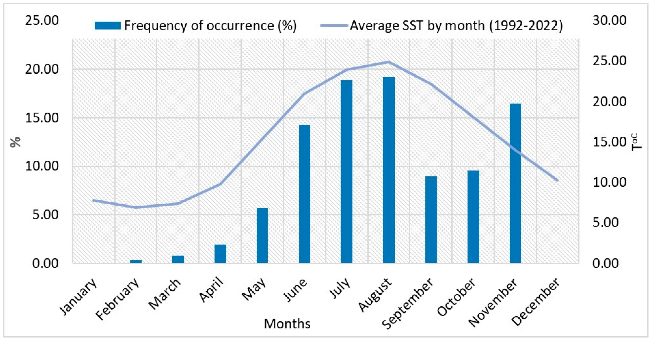
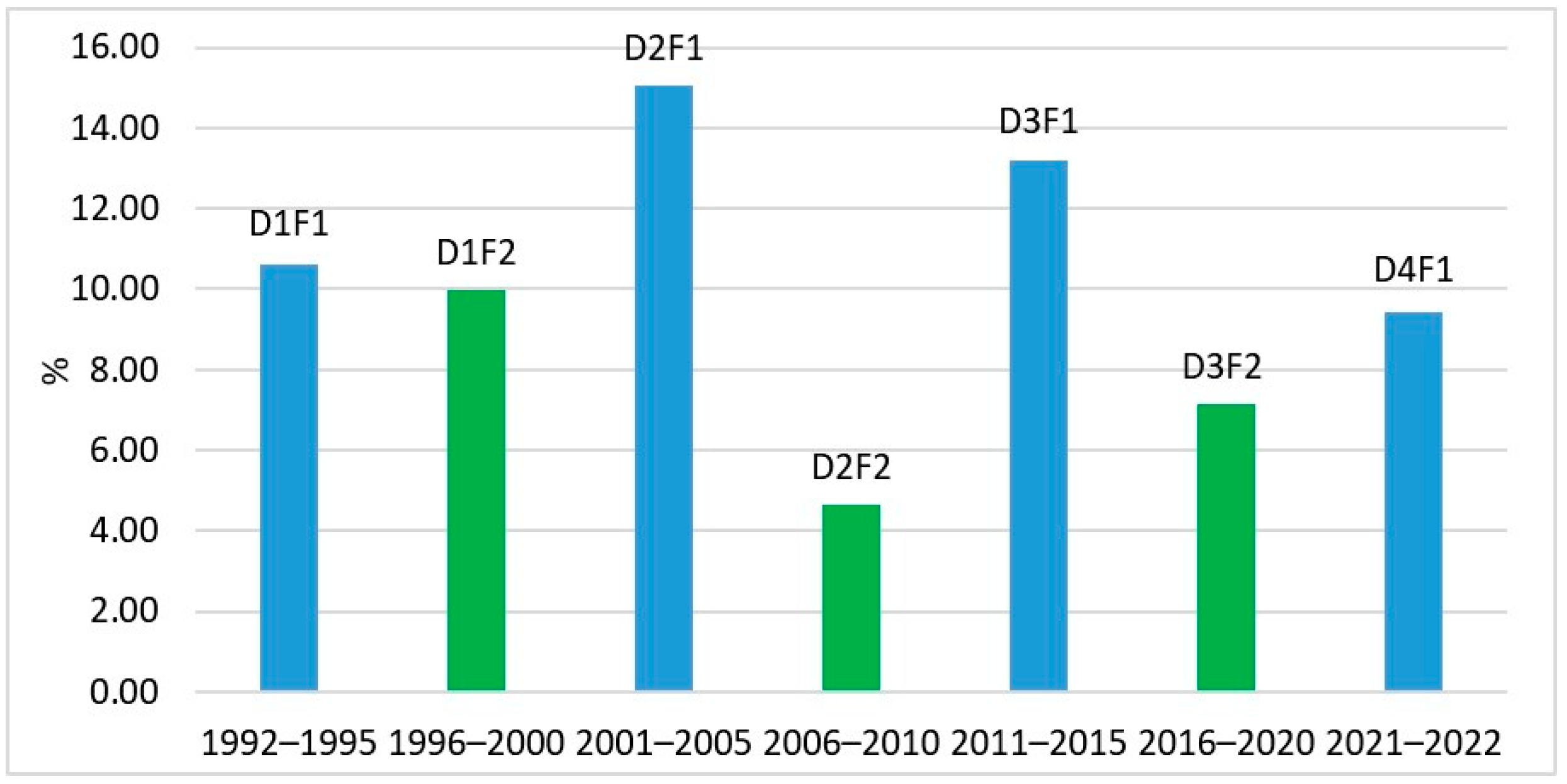
3.1. Tendencies in the Changes of L. polyedra Abundance, Biomass, Volume of Cells and Frequency of Occurrence in the Bulgarian Black Sea Waters

The maximum abundances of L. polyedra in Bulgarian Black Sea waters have changed over the years, with the following trend: y = 31.493x^−0.692; R² = 0.1783, and maximum biomasses by: y = 1987.7x^−0.756; R² = 0.1752.

At the beginning of the study period, in August 1992 in the Gulf of Varna, L. polyedra reached quantitative indicators describing the development of a bloom—an abundance of 1000 (mln. cells·m⁻³) and biomass 52,752.00 mg·m⁻³.

In the 1990s, L. polyedra continued to develop intensively with high biomass (≥1000 mg·m⁻³).

In the first and second decades of the 21st century, the maximum abundances and biomass of the species did not exceed 13 mln. cells·m⁻³ and 460 mg·m⁻³ (Figure 3).

A decrease in the average annual abundance and biomass of L. polyedra was observed for the period from 1992 to the present, following the trends y = 10.901x^−0.59; R² = 0.1973 and y = 663.14x^−0.673; R² = 0.6707, respectively (Figure 4).

A long-term tendency to reduce the volume of L. polyedra cells by y = −0.0368x³ + 2.4444x² − 96.898x + 55,285; R² = 0.2053 has been registered (Figure 4). These volumes in the 1990s averaged 54,035 μm³, while in the second decade of the 21st century, they decreased to an average of 45,457 μm³ (Figure 5).

Statistically significant differences were reported between the average abundance values of L. polyedra during the first decade of the studied period and the second and third decades (

Table 2. Multivariate analysis of average abundance (mln. cells·m⁻³), biomass (mg·m⁻³), volume of cells (µm³), and frequency of occurrence (%) of L. polyedra, 1992–2022 by decade.

Variable	$\overline{\mathit{x}}\pm \mathit{S}\mathit{D}$
	D1	D2	D3	D4
	(n = 38)	(n = 22)	(n = 28)	(n = 3)
Average abundance (mln. cells·m−3)	10.37 ± 28.78 a	1.75 ± 1.64 a	2.38 ± 1.99 a	2.62 ± 2.54
	R2 = 0.047; Sig.(p) = 0.043
Average biomass (mg·m−3)	553.40 ± 1525.57 a	93.69 ± 91.42 a	101.85 ± 87.20 a	124.01 ± 149.69
	R2 = 0.050; Sig.(p) = 0.013
Average volume of cell (µm3)	54,034.98 ± 6849.47 a	53,041.24 ± 6701.50 b	45,456.77 ± 10,846.40 ab	37,427.54 ± 16,852.03
	R2 = 0.223; Sig.(p) = 0.001
Frequency of occurrence (%)	24.93 ± 21.79	20.42 ± 18.13	18.91 ± 11.58	28.17 ± 13.38
	R2 = 0.026; Sig.(p) = 0.510

$\overline{x}$—mean values of the investigated variables; SD—standard deviation; R²—coefficient of determination; n—number of the observations; test: Post Hoc Tukey; D1—the first decade (1992–2000); D2—the second decade (2001–2010); D3—the third decade (2011–2020); D4—the fourth decade (2021–2022). Same superscripts within the row represent significant differences at the 0.05 level, as follows: ^a between investigated variables at D1 and the other decades; ^b between investigated variables at D2 and the other decades.

). The highest average abundance values (10.37 mln. cells·m⁻³) were observed during the first decade. The same tendency was observed regarding the biomass of L. polyedra. Again, statistically significant differences were reported in average biomass during the first decade of the studied period and the second and third decades, with the highest average biomass values (553.40 mg·m⁻³) observed during the first decade. The average values of the volume of cells during the first (54,034.98 µm³) and the second decade (53,041.24 µm³) differed significantly from those during the third decade (45,456.77 µm³). No statistically significant differences were reported in the frequency of occurrence of L. polyedra during the different decades.

For the entire period of study, L. polyedra has occurred with the highest abundances and biomass from July to October (

Table 3. Monthly development of L. polyedra abundance (mln. cells·m⁻³) and biomass (mln. cells·m⁻³), for the period 1992–2022.

Month	Max Abundance (mln. cells·m−3)	Average Abundance (mln. cells·m−3)	Min Abundance (mln. cells·m−3)	Max Biomass (mg·m−3)	Average Biomass (mg·m−3)	Min Biomass (mg·m−3)
2	0.10	0.08	0.06	5.42	4.55	3.67
3	20.00	11.46	2.93	769.30	458.21	147.12
4	1.24	0.39	0.08	70.24	21.09	1.94
5	8.14	2.29	0.04	460.18	130.29	2.08
6	13.33	2.60	0.03	762.13	146.11	1.52
7	81.44	3.11	0.05	4603.07	151.94	1.85
8	1000.00	13.15	0.05	52,752.00	686.72	1.40
9	40.08	5.45	0.05	2265.52	285.76	3.06
10	28.98	5.86	0.06	1528.81	298.17	3.55
11	20.00	2.40	0.05	906.83	128.27	2.08

) at an average sea water temperature of 23.60 °C.

A special feature was the intensive development of the species in March 1995 (Table 3) in the Varna Bay, a coastal zone where high values of total phytoplankton biomass are usually observed [64].

At depth, L. polyedra develops in the well-lit layer of water from 0 m to 18 m deep (Figure 5). The maxima of the development of the species were found at 0, 6, 14 and 18 m. Below this depth, the species occurs with relatively minimal concentrations (below 5 mln. cells·m⁻³) (Figure 6). The tendency with which the abundance of L. polyedra decreases in depth is with power trend line: y = 17.005x^−0.911; R² = 0.5551.

In the period 1992–2022, in Bulgarian Black Sea waters, the species had the highest frequency of occurrence (%) in 2000—29.68%, 2012—22.03%, 2016—19.15% and 2022—21.74% (Figure 7). The trend with which the frequency of occurrence (%) changes over the years is with power trend line: y = 2 × 10⁻⁵x⁶ − 0.0015x⁵ + 0.0556x⁴ − 0.9708x³ + 8.1448x² − 28.665x + 38.664; R² = 0.3322.

It was found that the population of the dinoflagellate L. polyedra develops from February to November (Figure 8). It has a low distribution during the cold months (February to April, mean SST 8.43 °C), while in the months of January and December, the species has not been recorded (Figure 8).

From May to November, the proportion of L. polyedra in phytoplankton samples is over 5%, with the highest proportion of occurrences being found in July (18.90%) and August (19.22%), when SST is higher than 23 °C (Figure 8).

The average abundances (mln. cells·m⁻³) and biomass (mg·m⁻³) of L. polyedra over five-year periods demonstrate a decrease in quantities until 2001–2005, after which there is an upward trend (Figure 9).

Statistically significant differences were found between the average values of the abundance and biomass of L. polyedra during the first and second five-year periods of D1 and D2 (

Table 4. Multivariate analysis of the average abundance (mln. cells·m⁻³), biomass (mg·m⁻³), volume of cells (µm³), and frequency of occurrence (%) of L. polyedra by the five-year periods over the decades.

Variable	D1		D2		D3
	Period (n)	$\overline{\mathit{x}}\pm \mathit{S}\mathit{D}$	Period (n)	$\overline{\mathit{x}}\pm \mathit{S}\mathit{D}$	Period (n)	$\overline{\mathit{x}}\pm \mathit{S}\mathit{D}$
Average abundance (mln. cells·m−3)	D1F1 (16)	19.61 ± 42.96 a	D2F1 (13)	0.97 ± 0.89 a	D3F1 (20)	2.22 ± 1.96
	D1F2 (22)	3.65 ± 5.29 a	D2F2 (9)	2.89 ± 1.84 a	D3F2 (8)	2.78 ± 2.14
Average biomass (mg·m−3)	D1F1 (16)	1035.50 ± 2277.40 b	D2F1 (13)	50.03 ± 45.63 b	D3F1 (20)	96.72 ± 89.51
	D1F2 (22)	202.78 ± 300.10 b	D2F2 (9)	156.74 ± 106.03 b	D3F2 (8)	114.68 ± 85.56
Average volume of cell (µm3)	D1F1 (16)	54,497.53 ± 5503.18	D2F1 (13)	52,301.22 ± 7254.58	D3F1 (20)	46,237.62 ± 10,572.75
	D1F2 (22)	53,698.58 ± 7794.01	D2F2 (9)	54,110.14 ± 6063.871	D3F2 (8)	43,504.68 ± 12,010.96
Frequency of occurrence (%)	D1F1 (16)	25.78 ± 17.63	D2F1 (13)	21.93 ± 16.51	D3F1 (20)	18.32 ± 9.52
	D1F2 (22)	24.32 ± 24.78	D2F2 (9)	18.24 ± 21.09	D3F2 (8)	20.38 ± 16.37

$\overline{x}$—mean values of the investigated variables; SD—standard deviation; R²-coefficient of determination; n—number of the observations; test: Post Hoc Tukey; D1F1—First five-year period of the first decade D1 (1992–1995); D1F2—Second five-year period of the first decade D1 (1996–2000); D2F1—First five-year period of the second decade D2 (2001–2005); D2F2—Second five-year period of the second decade D2 (2006–2010); D3F1—First five-year period of the third decade D3 (2011–2015); D3F2—Second five-year period of the third decade D3 (2016–2020). Same superscripts within the column represent significant differences at the 0.05 level, as follows: ^a between the average abundances over the decades; ^b between the average biomass over the decades.

). Regarding the average volume of cells and the frequency of occurrence of L. polyedra, no statistically significant differences were reported during the first and second five-year periods of the decades.

Tracking the frequency (%) of occurrence of L. polyedra for these periods, it was found that the proportion of occurrence of the species increased at the beginning of each decade. At the end of the decade, L. polyedra occurred with a lower percentage (Figure 10). It is possible that this periodicity is a consequence of the phenomenon recorded by Oguz et al. (2006) [65], that the periodicity in the cycles of NAO affects the enrichment of the surface (photic) water layer of the Black Sea with nutrients at the beginning of each decade.

Summarising the literature data for 1987–1992 [19,33] and the data from our study (1992–2022), it is possible to determine the Bulgarian water areas with maximum abundances and biomass of the potentially toxic species L. polyedra (

Table 5. The maximum values for the species in Bulgarian waters between 1987 and 2022: offshore (to 3 n.m.), open sea (>3 n.m.).

№	Regions	Distance from the Shore	Max of Abundance (mln. cells·m−3)	Max of Biomass (mg·m−3)
1	Biala	offshore	3.35	70.96
2	Albena	offshore	0.16	8.79
3	Balchik	offshore	4.91	121.48
4	Beloslav lake	offshore	11.59	799.35
5	Burgas bay	offshore	40.08	2114.22
6	cape Emine	offshore	18.29	965.08
7	cape Emine	open sea	14.67	674.27
8	cape Galata	offshore	81.44	4603.07
9	cape Galata	open sea	9.43	532.90
10	cape Kaliakra	offshore	9.01	191.15
11	cape Kaliakra	open sea	1.19	67.49
12	cape Maslen	offshore	0.55	31.25
13	Dvoinitca	offshore	0.43	21.41
14	Ilandzhik	offshore	1.51	85.36
15	Kamchia	offshore	0.34	19.00
16	Krapec	offshore	0.26	9.91
17	Rusalka	offshore	2.43	93.32
18	Shabla	offshore	5.67	160.28
19	Sozopol	offshore	2.72	104.73
20	Varna bay	offshore	1600.00	84,403.20
21	Varna lake	offshore	8.14	460.18
22	Varvara	offshore	0.66	37.58
23	Veleka	offshore	1.94	87.86

).

L. polyedra developed most intensively in the eutrophic waters of Varna Bay, Burgas Bay, and Cape Galata (offshore). In all other water areas, the species is with maximum abundance of 18.29 mln. cells·m⁻³ and maximum biomass of 965.08 mg·m⁻³ (Table 5).

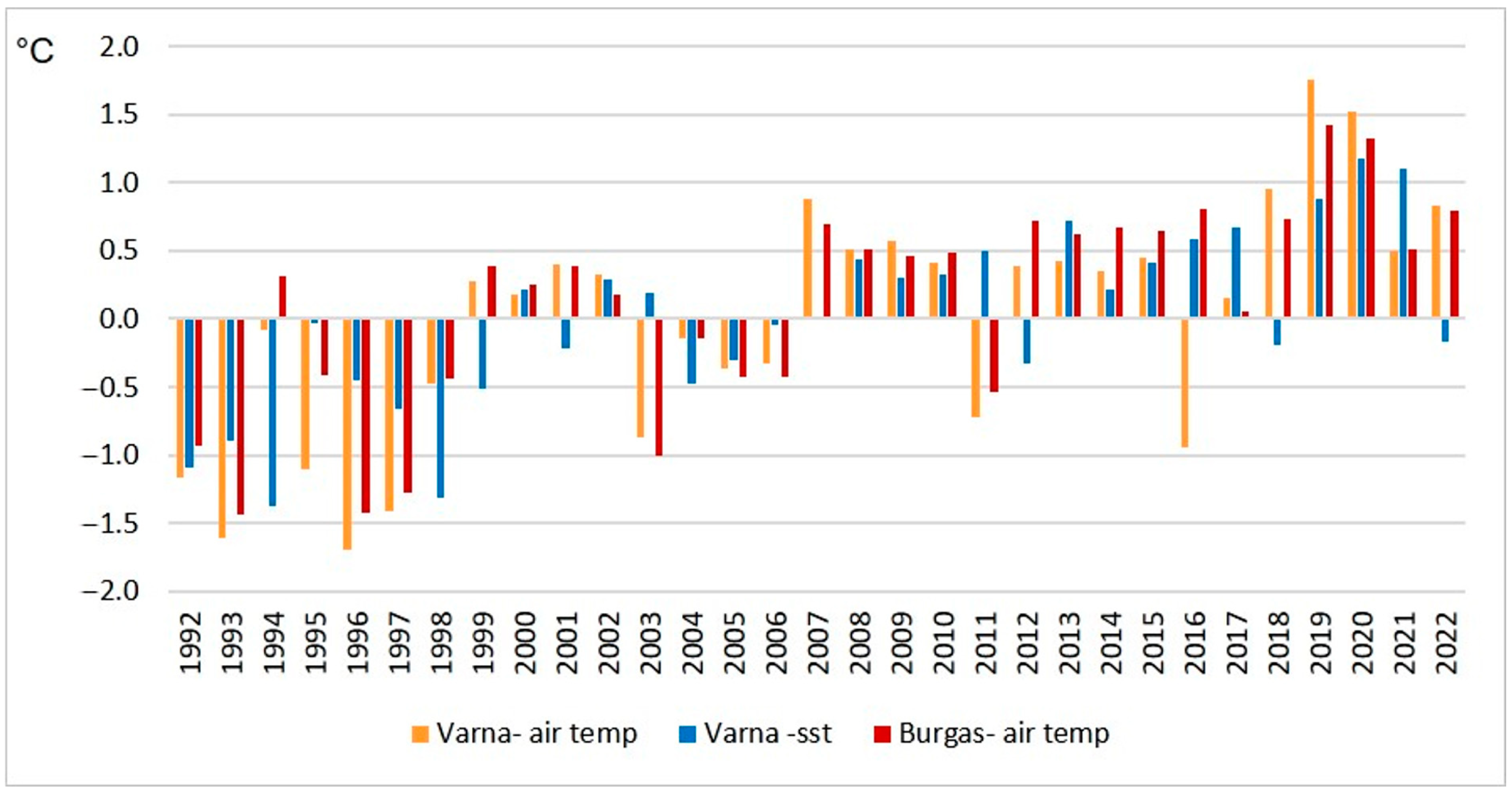
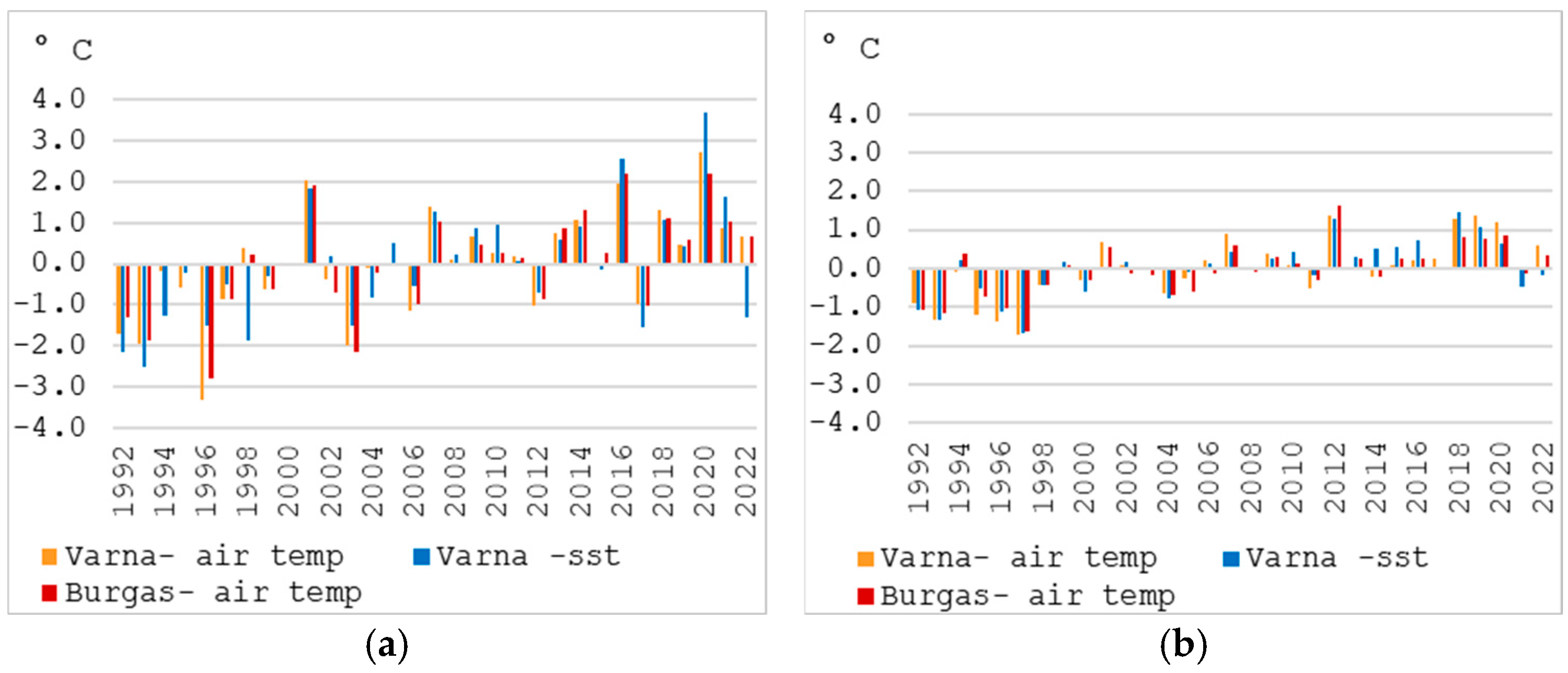
3.2. Climate Characteristics and Observed Changes in Air and Sea Surface Temperature (1992–2022)

According to the Koppen climate classification [66], most Bulgarian Black Sea coast has climatic type Cfa (warm temperate climate, fully humid with a hot summer). Only the southernmost parts of the coastline fall within the Cs (warm temperate climate with dry summer) climate-type zone [67]. The annual cycle of the air temperature is characterized by a minimum in January when average monthly temperatures drop to 2–3 °C, and a maximum in August, reaching 23–24 °C. The average annual air temperature for the study period (1992–2022) is approximately 13 °C. The SST is higher than the air temperature, especially during the colder part of the year.

Long-term temperature changes are characterized by a positive statistically significant trend, with values of 0.6–0.7 °C per decade for annual air temperatures and 0.5 °C per decade for annual SST. The trend during the cold part of the year (November–April) is 0.8 °C per decade (both for air and sea surface temperatures) while in the warm part (May–October) the trend is 0.6–0.7 °C per decade.

The analysis of temperature anomalies calculated relative to the average for the period 1992–2022 for annual air and sea surface temperatures, shows that most of the study period exhibits positive temperature anomalies, while negative anomalies are mainly observed up until 1998 (Figure 11). A relatively cold period was observed from 2002 to 2006.

A similar occurrence of negative and positive temperature anomalies was established for the cold (November–April) and warm (May–October) parts of the year (Figure 12a,b). After 2000, the years with negative anomalies for both the cold and warm half of the year were 2012 and 2017. The notable years are 2016 and 2020 also, with the highest temperature anomaly for the cold half of the study period—over 2 °C. For water, the temperature in 2020 was 3.7 °C higher than the 1992–2022 average.

The highest positive anomalies for the warm half of the year were recorded in 2012, as well as for the period 2018–2020. The first decade of the study period is marked by negative temperature anomalies for May–October (Figure 12).

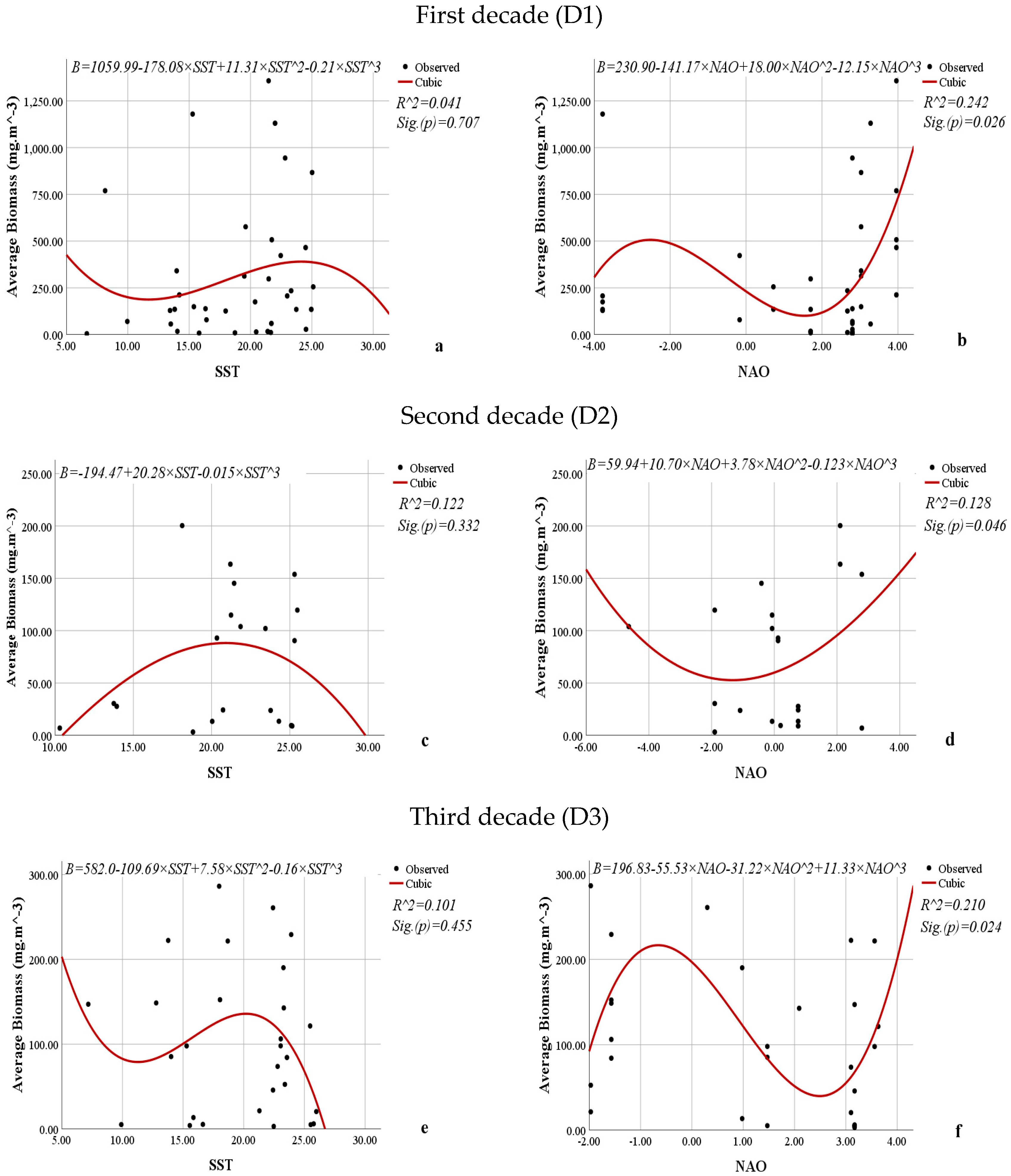
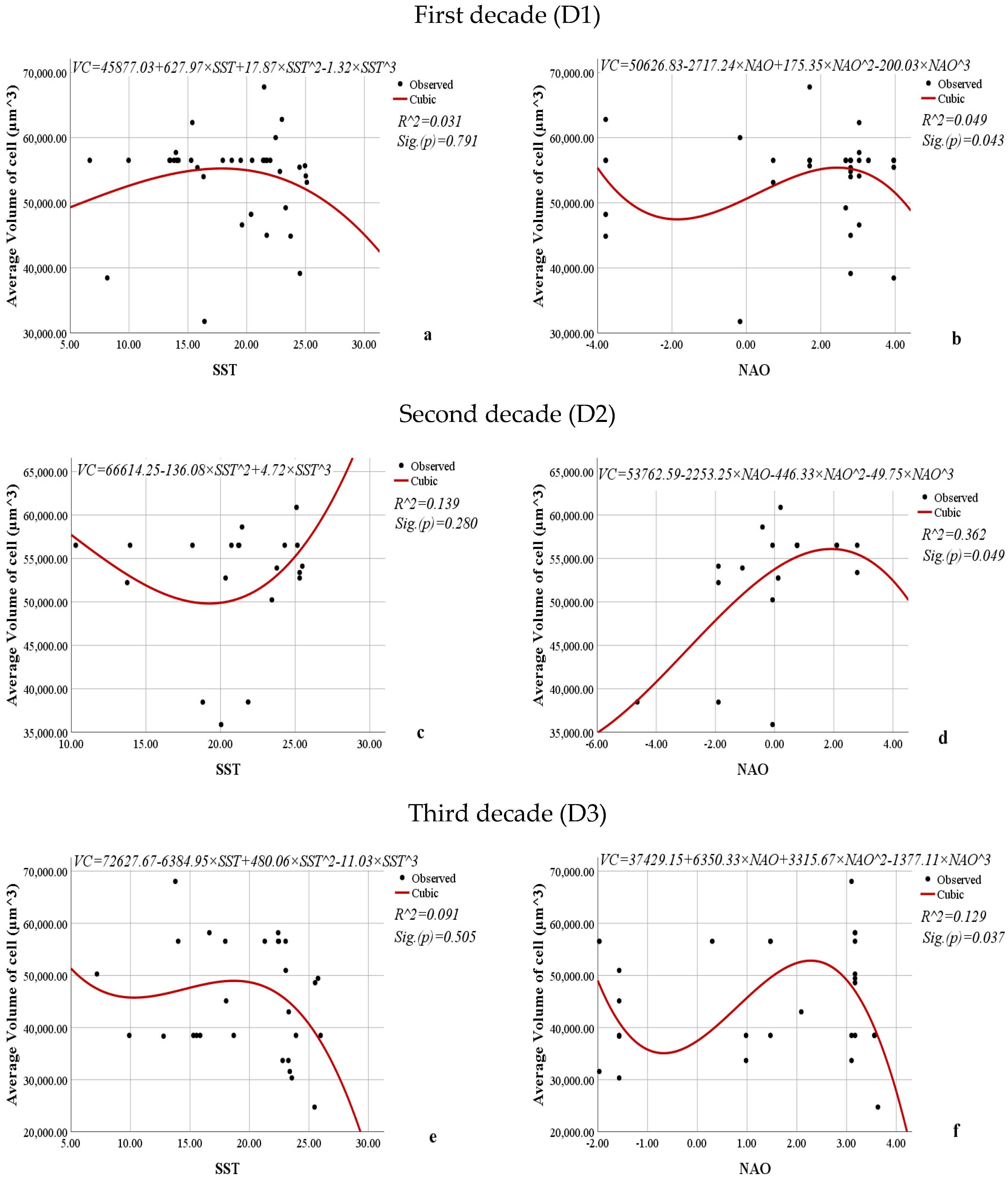
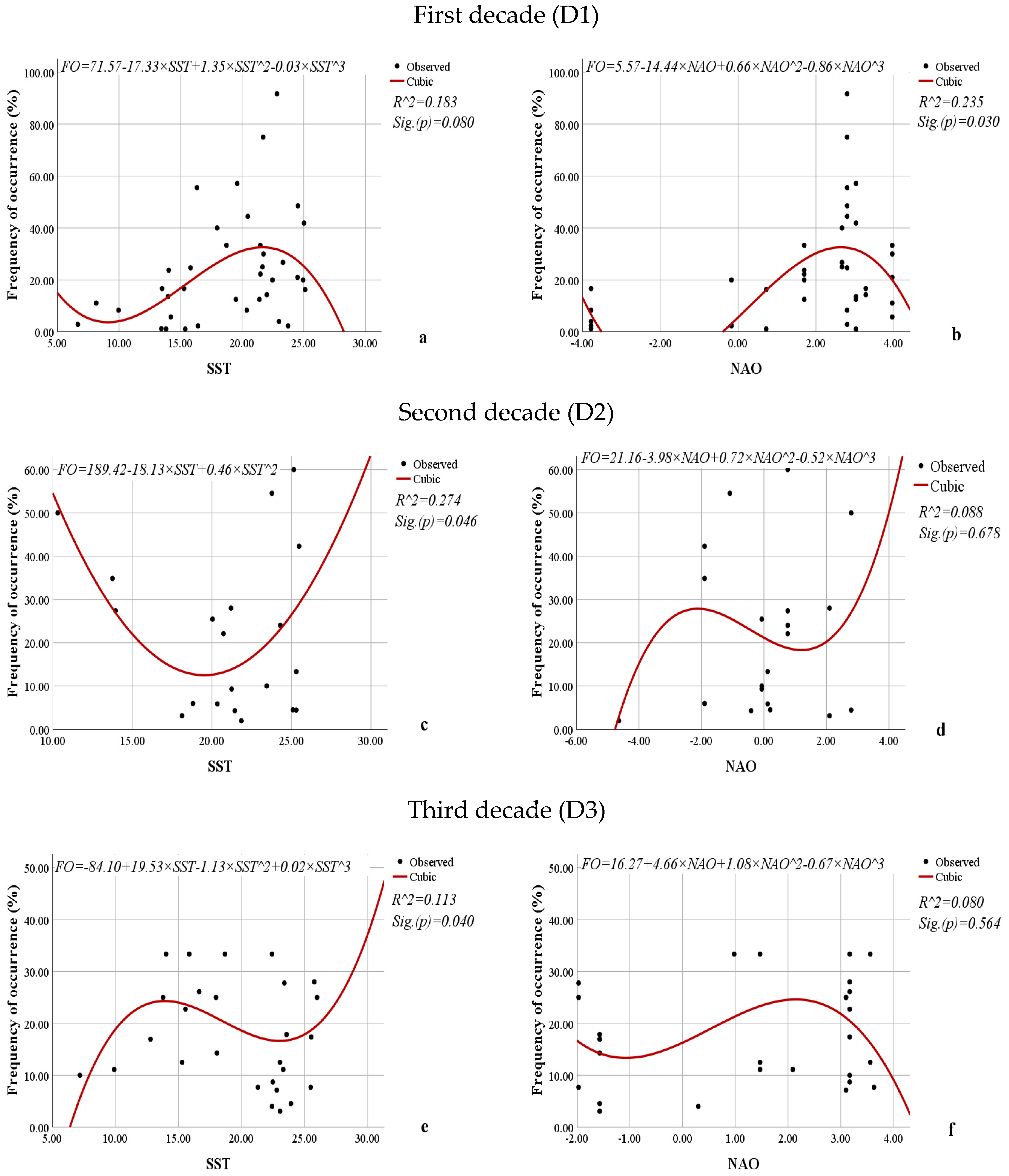
3.3. Relationship Between the Average Abundance (mln. cells·m⁻³), Biomass (mg·m⁻³), Volume of Cells (µm³), Frequency of Occurrence (%) of L. polyedra, and the Sea Surface Temperature and North Atlantic Oscillation Indices

For greater clarity, the relationships between average abundance, biomass, the volume of cells, and the frequency of occurrence of L. polyedra and SST and NAO were investigated for the individual decades. The outliers were removed from the sample to achieve higher accuracy of the developed models. The results show weak correlations between all the monitored parameters and SST and NAO (

Table 6. Bivariate correlation between the average abundance (mln. cells·m⁻³), biomass (mg·m⁻³), volume of cells (µm³), frequency of occurrence (%) of L. polyedra, and the SST and NAO by decade.

n = 88	D1		D2		D3
	SST	NAO	SST	NAO	SST	NAO
Average abundance (mln. cells·m−3)	0.118	0.110	0.242	0.038	0.051	−0.300
Average biomass (mg·m−3)	0.172	0.090	0.216	0.155	−0.085	−0.303
Average volume of cell (µm3)	0.003	0.037	0.056	0.554 *	−0.188	0.067
Frequency of occurrence (%)	0.374 *	0.374 *	−0.152	0.103	−0.054	0.162

* Correlation is significant at the 0.05 level (2-tailed); SST—sea surface temperature; NAO—North Atlantic Oscillation indices.

). The correlation between the frequency of occurrence and SST and NAO for the first decade (0.374), as well as between the average volume of cells and NAO for the second decade (0.554), is moderate and statistically significant.

The influence of SST and NAO on average abundance, biomass, the volume of cells, and the frequency of occurrence of L. polyedra by decade was examined through the obtained nonlinear regression models (Figure 13, Figure 14, Figure 15 and Figure 16). The calculated models showing the relationship between SST and the average abundance of L. polyedra for the three decades are statistically insignificant (Figure 12). The coefficients of determination (0.036, 0.132, and 0.067) indicate that only 3.6 to 13.2% of the variations in abundance over the three decades are due to the influence of SST.

In turn, the obtained models showing the relationship between NAO and the average abundance of L. polyedra over the three decades are statistically significant (0.013, 0.044, 0.018). NAO weakly to moderate (R² = 0.275, 0.151, 0.336) influence the average abundance of L. polyedra over the three decades.

Similar results were obtained for the models showing the relationship between SST and the average biomass of L. polyedra over the three decades (Figure 14). The models are statistically insignificant (0.707, 0.332, 0.455). From the coefficients of determination (0.041, 0.122, and 0.101), it can be concluded that 4.1% to 12.2% of the variations in the average biomass of L. polyedra over the three decades are due to the influence of SST. The NAO has a weak to moderate (R² = 0.242, 0.128, 0.210) but statistically significant (0.026, 0.046, 0.024) effect on the average biomass of L. polyedra over the three decades.

The models expressing the relationships between SST and the average volume of cells of L. polyedra are statistically insignificant (0.791, 0.280, 0.505) for all three decades, indicating that SST does not significantly influence the average volume of cells of L. polyedra (Figure 15).

On the other hand, NAO significantly influences the average volume of cells of L. polyedra across all decades (0.043, 0.049, 0.037). The coefficients of determination (0.049, 0.362, 0.129) show that during the first decade, only 4.9% of the variations in the volume of cells of L. polyedra result from the influence of NAO. During the third decade, 12.9% of the variations in the volume of cells of L. polyedra are attributed to NAO. The impact of NAO is most pronounced in the second decade, as 36.2% of the variations in the volume of cells of L. polyedra result from its influence.

When examining the relationships between SST, NAO, and the frequency of occurrence of L. polyedra over the decades, contradictory results are obtained (Figure 16). For the first decade, the influence of SST is statistically insignificant (0.080), while the impact of NAO is statistically significant (0.030). According to the coefficient of determination (0.235), 23.5% of the variations in the frequency of occurrence of L. polyedra during the first decade are due to the influence of NAO.

According to the models obtained for the second and third decades, the influence of SST is statistically significant (0.046, 0.040), while the impact of NAO is statistically insignificant (0.678, 0.564). The influence of SST is more pronounced during the second decade, with 27.4% of the variations in the frequency of occurrence of L. polyedra due to its impact.

4. Discussion

Blooms of L. polyedra in Bulgarian marine waters were observed exclusively in the late 1980s and early 1990s (Figure 2). Since the early 1990s, blooms of L. polyedra have not been observed, and higher concentrations of the species have been recorded during the warmer months only (Figure 3 and Figure 8, Table 3).

This is consistent with the trend of overall reduction in the concentration of biogenic elements [21,68]. “The decreasing DIN (Dissolved Inorganic Nitrogen) significantly affects the decrease in the abundance and biomass of Dinophyceae” [21] (p. 1).

At the same time, long-term temperature changes are being recorded in Bulgarian marine waters, characterized by a positive statistically significant trend, with values of 0.6–0.7 °C per decade for annual air temperatures and 0.5 °C per decade for annual SST. The trend during the cold part of the year (November–April) is 0.8 °C per decade (both for air and sea surface temperatures) while in the warm part (May–October) the trend is 0.6–0.7 °C per decade.

In the 1990s, when temperature anomalies were predominantly negative, there was a more intensive development of the species (Figure 3, Figure 4, Figure 11 and Figure 12).

Over the past three decades, numerous scientific publications have reported a trend of decreasing phytoplankton abundance, biomass, and the number and intensity of phytoplankton blooms in the Bulgarian marine waters of the Black Sea [20,21,36,37,38]. The number of recorded phytoplankton species causing harmful algal blooms in Bulgarian Black Sea waters has also decreased [21].

Similarly, during our study, we also observed a trend of decreasing abundance, biomass, and distribution of the dinoflagellate L. polyedra (Figure 3 and Figure 7).

After 1992, when L. polyedra was last recorded with a high abundance (1000.00 mln. cells·m⁻³) and biomass (52.752 mg·m⁻³), (“red tide”), the maximum concentrations in Bulgarian marine waters have not exceeded 115.25 mln. cells·m⁻³ (observed in August 1994 in the waters of Varna Bay), and in recent years they have been steadily lower (Figure 3).

During this study, a trend of decreasing cell volumes of the species was also observed. Most likely, this phenomenon is related to the established trend of increasing SST and decreasing the amounts of nutrients [21] (Figure 5).

The results of the statistical analysis on the influence of the climate parameters NAO and SST on the population dynamics of L. polyedra indicate that changes in SST have a weak to negligible impact on the quantitative development (abundance, biomass) of the species (up to 12.2–13.2% of the variations in abundance and biomass are attributed to SST influence). The NAO cycles have a stronger impact on L. polyedra, accounting for 12.8% to 24.2% of the variations in abundance and biomass of the species across different decades (Figure 13 and Figure 14). This appears to be due to the impact of NAO cycles on the physical and biogeochemical properties of Black Sea waters [65].

We found that the NAO has a more significant impact on the morphological characteristics of the species, such as the volume of its cells (Figure 14). NAO significantly influences the average volume of cells of L. polyedra across all decades (0.043, 0.049, 0.037). The impact of NAO is most pronounced in the second decade, as 36.2% of the variations in the volume of cells of L. polyedra result from its influence (Figure 15).

The correlation between the frequency of occurrence and SST and NAO for the first decade (0.374), as well as between the average volume of cells and NAO for the second decade (0.554), is moderate and statistically significant.

L. polyedra predominantly develops in coastal waters at depths of up to 18 m. Vertically, it is found in higher concentrations either at the surface or in the bottom layer, where nutrients are more readily available (Figure 6).

As a result of the conducted analysis, we determined that the Bulgarian marine areas where L. polyedra develops with high densities and biomass are Varna Bay, Cape Galata (offshore), and Burgas Bay (Table 5).

The Varna Bay is one of the marine “hot spots” along the Bulgarian Black Sea coast [21]. “The quality of sea water in the bay is largely determined by the water exchange with the Varna Lake from which eutrophic waters constantly flow in” [69] (p. 71).

On the other hand, the development of phytoplankton in the coastal area near Cape Galata (offshore) is influenced by the currents from the eutrophied Varna Lake and Varna Bay [70].

The waters of Burgas Bay are also strongly influenced by waste emissions from various industries, petroleum derivatives, and wastewater from livestock farms as well as the densely populated residential areas [71].

Since L. polyedra forms cysts after blooming, which are preserved in the sediment [8,9,33], we can expect that under favorable environmental conditions, the species will reach high abundance and biomass again in areas where it has been previously recorded during a bloom.

At the same time, the immense potential of the dinoflagellate L. polyedra to cause red tides under suitable conditions, which threaten both the ecosystem balance of the Black Sea and human health (due to toxins produced by the species), was demonstrated by the intense bloom of the species (56,100 million cells·m⁻³) observed in October 2020 in the anthropogenically influenced waters of Odessa Bay [15].

“The presence of such high abundances is primarily associated with the “closeness” of this area of the Odesa Bay. It is characterized by a limited water exchange with the open water area of the bay, which contributes to an increase of the trophic state of the water.” [15] (p. 4).

It seems that controlling the blooms of L. polyedra is directly dependent on managing coastal pollution sources, as they have the strongest impact on the nutrient supply to the coastal areas and bays where this dinoflagellate is typically found in high concentrations.

5. Conclusions

The results of the present study seem to indicate that the development of the dinoflagellate Lingulodinium polyedra depends on the depth of the water body and the influence of coastal pollution sources. As the distance from the shore increases, the abundance and biomass of the species decrease. This is most likely related to the characteristics of its life cycle. Under unfavorable conditions in the coastal areas, the process of cyst formation intensifies.

On the one hand, the quantitative indicators of L. polyedra in Bulgarian marine waters, such as the abundance, biomass and volume of cells of the species show a persistent trend of reduction. On the other hand, this characteristic demonstrates a reduced threat to hydrobionts from toxin intoxication.

The established influence of climatic factors such as NAO and SST on the species population varies from weak to moderate, with the correlation with NAO cycles being better expressed. This is probably due to the stronger impact of changes in winter temperatures of the 18 m surface water layer, where the species mainly develops. Monitoring of potentially toxic species (including L. polyedra) in the Bulgarian waters of the Black Sea remains a priority for protecting human health.

References

1. Guiry, M.D.; Guiry, G.M. World-Wide Electronic Publication, National University of Ireland, Galway. AlgaeBase. Available online: http://www.algaebase.org (accessed on 12 December 2024).
2. Petrova, V.J. Composition and quantitative distribution of phytoplankton in Varna Bay. Proc. Bot. Inst. BAS 1960, 7, 247–277. (In Bulgarian) [Google Scholar]
3. Petrova, V.J. The phytoplankton of Lake Varna. Proc. Cent. Sci. Res. Inst. Fish Resour.-Varna 1961, 1, 183–220. (In Bulgarian) [Google Scholar]
4. Faust, M.; Gulledge, R. Identifying Harmful Marine Dinoflagellates. Contrib. U. S. Natl. Herb. 2002, 42, 1–144. Available online: http://www.jstor.org/stable/23493225 (accessed on 8 July 2024).
5. Kofoid, C.A. Dinoflagellata of the San Diego region, IV. The genus Gonyaulax, with notes on its skeletal morphology and a discussion of its generic and specific characters. Univ. Cal. Publ. Zool. 1911, 8, 187–269. [Google Scholar]
6. Kiselev, I.A. Dinoflagellata of the Seas and Fresh Waters of the USSR. Determinants of Fauna of the USSR; Zoological Institute of the Academy of Sciences of the USSR: Moscow, Russia, 1950; pp. 1–280. (In Russian) [Google Scholar]
7. Nielsen, L.T.; Kiørboe, T. Feeding currents facilitate a mixotrophic way of life. ISME J. 2015, 9, 2117–2127. [Google Scholar] [CrossRef] [PubMed] [PubMed Central]
8. Taylor, F.J.R. The Biology of Dinoflagellates; Blackwell: Oxford, UK, 1987; pp. 1–785. [Google Scholar]
9. Prego, R.; Bao, R.; Varela, M.; Carballeira, R. Naturally and Anthropogenically Induced Lingulodinium polyedra Dinoflagellate Red Tides in the Galician Rias (NW Iberian Pterenkoeninsula). Toxins 2024, 16, 280. [Google Scholar] [CrossRef] [PubMed]
10. Lundholm, N.; Churro, C.; Escalera, L.; Fraga, S.; Hoppenrath, M.; Iwataki, M.; Larsen, J.; Mertens, K.; Moestrup, Ø.; Murray, S.; et al. (Eds.) (2009 Onwards). IOC-UNESCO Taxonomic Reference List of Harmful Micro Algae. Lingulodinium polyedra (F. Stein) J.D. Dodge, 1989. Available online: https://www.marinespecies.org/hab/aphia.php?p=taxdetails&id=233592 (accessed on 29 October 2024).
11. Amorim, A.; Palma, A.S.; Sampayo, M.A.; Moita, M.T. On a Lingulodinium polyedrum Bloom in Setúbal Bay, Portugal. In Harmful Algal Blooms 2000; Hallegraef, G.M., Blackburn, S.I., Bolch, C.J., Lewis, R.J., Eds.; Intergovernmental Oceanographic Commission of UNESCO: Hobart, Australia, 2001; pp. 133–136. [Google Scholar]
12. Meave del Castillo, M.E.; Zamudio-Resendiz, M.E. Planktonic algal blooms from 2000 to 2015 in Acapulco Bay, Guerrero, Mexico. Acta Bot. Mex. 2018, 125, 61–93. [Google Scholar] [CrossRef]
13. Mertens, K.N.; Retho, M.; Manach, S.; Zoffoli, M.L.; Doner, A.; Schapira, M.; Bilien, G.; Séchet, V.; Lacour, T.; Robert, E.; et al. An unprecedented bloom of Lingulodinium polyedra on the French Atlantic coast during summer 2021. Harmful Algae 2023, 125, 102426. [Google Scholar] [CrossRef] [PubMed]
14. Zernov, S.A. On the problem of studying life in Black Sea. Proc. Emp. Acad. Sci. 1913, 32, 1–310. (In Russian) [Google Scholar]
15. Terenko, G.; Krakhmalnyi, A. Red tide of the Lingulodinium polyedrum (Dinophyceae) in Odessa Bay (Black Sea). Turk. J. Fish. Aquat. Sci. 2022, 22, TRJFAS20312. [Google Scholar] [CrossRef]
16. Moncheva, S.P. On the thermohaline characteristics of development of some massive phytoplankton species from the northern part of the Bulgarian coast. Oceanology 1991, 21, 14–20. (In Bulgarian) [Google Scholar]
17. Dzhembekova, N.; Moncheva, S. Recent trends of potentially toxic phytoplankton species along the Bulgarian Black Sea area. In Proceedings of the 12 International Conference on Marine Science and Technology “Black Sea 2014”, Varna, Bulgaria, 25–27 September 2014; pp. 321–329. [Google Scholar]
18. Ryabushko, L.I. Potentially Dangerous Microalgae of the Azov-Black Sea Basin; ECOSI–Hydrophysics: Sevastopol, Ukraine, 2003; pp. 1–288. (In Russian) [Google Scholar]
19. Velikova, V.; Moncheva, S.; Petrova, D. Phytoplankton dynamics and Red Tides (1987–1997) in the Bulgarian Black Sea. Water Sci. Technol. 1999, 39, 27–36. [Google Scholar] [CrossRef]
20. Oguz, T.; Velikova, V. Abrupt transition of the northwestern Black Sea shelf ecosystem from a eutrophic to an alternative pristine state. Mar. Ecol. Prog. Ser. 2010, 405, 231–242. Available online: http://www.jstor.org/stable/24873891 (accessed on 2 July 2022). [CrossRef]
21. Klisarova, D.; Gerdzhikov, D.; Nikolova, N.; Gera, M.; Veleva, P. Influence of Some Environmental Factors on Summer Phytoplankton Community Structure in the Varna Bay, Black Sea (1992–2019). Water 2023, 15, 1677. [Google Scholar] [CrossRef]
22. Valkanov, A. Catalogue of Our Black Sea Fauna; State Publishing House “Science and Art”: Sofia, Bulgaria, 1957; pp. 1–62. (In Bulgarian) [Google Scholar]
23. Petrova, V.Y. Phytoplankton in the Black Sea in front of the Bulgarian coast during the period 1958–1960. Proc. Inst. Fish Farming Fish.-Varna 1964, 5, 5–32. (In Bulgarian) [Google Scholar]
24. Petrova, V.Y. Peculiarities in the development of phytoplankton in the Black Sea in front of the Bulgarian coast in 1961–1963. Proc. Res. Inst. Fish. Oceanogr.-Varna 1965, 6, 63–74. (In Bulgarian) [Google Scholar]
25. Petrova, V. Phytoplankton in the Black Sea in front of the Bulgarian coast for the period 1954–1957. Proc. Cent. Res. Inst. Fish Farming Fish.-Varna 1963, 3, 31–60. (In Bulgarian) [Google Scholar]
26. Moncheva, S. Phytoplankton in the food of cultured mussels Mytilus galloprovicialis Lam. in the area of Cape Kaliakra. Proc. Inst. Fish Resour.-Varna 1983, 20, 145–152. (In Bulgarian) [Google Scholar]
27. Marasović, I.; Pucher-Petković, T.; Petrova-Karadjova, V. Prorocentrum minimum (Dinophyceae) in the Adriatic and Black Seas. J. Mar. Biol. Assoc. U. K. 1990, 70, 473–476. [Google Scholar] [CrossRef]
28. Petrova-Karadjova, V. Phytoplankton blooms in the Black Sea. Sci. Rep. Sci. Dev. Contemp. Social. Pract. 1979, 2, 8–12. (In Bulgarian) [Google Scholar]
29. Petrova-Karadjova, V.J. Changes in the planktonic flora in the Bulgarian Black Sea waters under the influence of eutrophication. Proc. Inst. Fish Resour. Varna 1984, 21, 105–112. (In Bulgarian) [Google Scholar]
30. Petrova-Karadjova, V.J. The “red tide” of Prorocentrum micans Ehr. and Exuviaella cordata Ost. in the Bay of Varna in November 1984. Hydrobiology 1985, 26, 70–78. (In Bulgarian) [Google Scholar]
31. Temniskova, D. Assoc. Prof. Vyara Petrova-Karadzhova: A life dedicated to the sea. In memory of the 75th anniversary of her birth. Phytol. Balc. 2005, 11, 103–118. Available online: http://www.bio.bas.bg/~phytolbalcan/PDF/11_2/11_2_01_Temniskova.pdf (accessed on 25 June 2024).
32. Mee, L.D. The Black Sea in a crisis: A need for concerted international action. Ambio 1992, 21, 278–285. [Google Scholar]
33. Moncheva, S. On some biological aspects of the “blooming” phenomena. In Proceedings of the Scientific-Practical Conference, Status of Research, Rational Utilization and Protection of Natural Resources of the Varna Region, Varna, Bulgaria, 30 October 1989; pp. 110–121. (In Bulgarian). [Google Scholar]
34. Oguz, T.; Abaza, V.; Akatov, V.; Aktan, Y.; Arashkevich, E.; Birkun, A.; Boicenco, L.; Chikina, M.V.; Cociasu, A.; Daskalov, G.M.; et al. State of the Environment of the Black Sea (2001–2006/7); Black Sea Commission Publications: Istanbul, Turkey, 2008; pp. 1–421. ISBN 978-9944-245-33-3. [Google Scholar]
35. Alexandrov, B.; Krutov, A.; Korshenko, A.; Lavrova, O.; Raykov, V.; Ivanova, P.; Dencheva, K.; Antonidze, E.; Golumbeanu, M.; Gvilava, M.; et al. State of the Environment of the Black Sea (2009–2014/5); Krutov, A., Ed.; Black Sea Commission Publications: Istanbul, Turkey, 2019; pp. 1–811. ISBN 978-605-84837-0-5. [Google Scholar]
36. Shtereva, G.; Velikova, V.; Doncheva, V. Human impact on marine water nutrients enrichment. J. Environ. Prot. Ecol. 2015, 16, 40–48. [Google Scholar]
37. Moncheva, S.; Doncheva, V.; Kamburska, L. On the long-term response of harmful algal blooms to the evolution of eutrophication off the Bulgarian Black Sea coast: Are the recent changes a sign of recovery of the ecosystem-the uncertainties. In Proceedings of the IX International Conference on Harmful Algal Blooms, Hobart, Tasmania, 7–11 February 2000; UNESCO-IOC: Paris, France, 2001; pp. 177–182. [Google Scholar]
38. Moncheva, S.; Slabakova, V.; Doncheva, V. Dominant habitat types in the water column—Phytoplankton. In Initial Assessment of the State of the Marine Environment, According to Article 8 of the WFD and the NOEMS; Publication of Institute of Oceanology: Varna, Bulgaria, 2013; pp. 168–180. (In Bulgarian) [Google Scholar]
39. Mee, L.D.; Friedrich, J.; Gomoiu, M.T. Restoring the Black Sea in Times of Uncertainty. Oceanography 2005, 18, 32–43. [Google Scholar] [CrossRef]
40. Zaitzev, Y.P. Impact of eutrophication on the Black Sea fauna. Gen. Fish. Counc. Mediterr. Stud. Rev. 1993, 64, 63–86. [Google Scholar]
41. Bruno, M.; Gucci, P.M.; Pierdominici, E.; Ioppolo, A.; Volterra, L. Presence of saxitoxin in toxic extracts from Gonyaulax polyedra. Toxicon 1990, 28, 1113–1116. [Google Scholar] [CrossRef] [PubMed]
42. Wang, D. Neurotoxins from Marine Dinoflagellates: A Brief Review. Mar. Drugs 2008, 6, 349–371. [Google Scholar] [CrossRef]
43. Lee, J. Environmental Bloom of Lingulodinium polyedrum in Southern California: Potential Health Risks. Master’s Thesis, University of California, San Diego, CA, USA, 2015. Available online: https://escholarship.org/uc/item/3zb9b1rp (accessed on 20 February 2022).
44. Paz, B.; Riobó, P.; Fernández, M.L.; Fraga, S.; Franco, J.M. Production and release of yessotoxins by the dinoflagellates Protoceratium reticulatum and Lingulodinium polyedrum in culture. Toxicon 2004, 44, 251–258. [Google Scholar] [CrossRef] [PubMed]
45. Howard, M.D.A.; Smith, G.J.; Kudela, R.M. Phylogenetic relationships of yessotoxin-producing dinoflagellates based on the large subunit and internal transcribed spacer ribosomal DNA domains. Appl. Environ. Microbiol. 2009, 7, 54–63. [Google Scholar] [CrossRef] [PubMed]
46. Knechtges, P. Food Safety: Theory and Practice; Jones & Bartlett Learning: Bulrington, VT, USA, 2012; pp. 1–459. [Google Scholar]
47. Stobo, L.A.; Lewis, J.; Quilliam, M.A.; Hardstaff, W.R.; Gallacher, S.; Webster, L.; Smith, E.; McKenzie, M. Detection of Yessotoxin in UK and Canadian Isolates of Phytoplankton and Optimization and Validation of LC-MS Methods; Bates, S., Ed.; Gulf Fisheries Centre: Moncton, NB, Canada, 2003; pp. 8–14.
48. Pistocchi, R.; Guerrini, F.; Pezzolesi, L.; Riccardi, M.; Vanucci, S.; Ciminiello, P.; Dell’Aversano, C.; Forino, M.; Fattorusso, E.; Tartaglione, L.; et al. Toxin Levels and Profiles in Microalgae from the North-Western Adriatic Sea—15 Years of Studies on Cultured Species. Mar. Drugs 2012, 10, 140–162. [Google Scholar] [CrossRef] [PubMed]
49. Huang, S.; Mertens, K.N.; Derrien, A.; David, O.; Shin, H.H.; Li, Z.; Cao, X.; Cabrini, M.; Klisarova, D.; Gu, H. Gonyaulax montresoriae sp. nov. (Dinophyceae) from the Adriatic Sea produces predominantly yessotoxin. Harmful Algae 2025, 141, 102761. [Google Scholar] [CrossRef]
50. Granéli, E.; Tuner, J.T. Ecology of Harmful Algae; Springer: Berlin/Heidelberg, Germany, 2006; pp. 1–413. [Google Scholar]
51. Yasakova, O.N. Seasonal dynamics of potentially toxic and harmful species of planktonic algae in Novorossiysk Bay (Black Sea). Biol. Sea 2013, 39, 98–105. (In Russian) [Google Scholar]
52. Morton, S.L.; Vershinin, A.; Leighfield, T.; Smith, L.; Quilliam, M. Identification of yessotoxin in mussels from the Caucasian Black Sea Coast of the Russian Federation. Toxicon 2007, 50, 581–584. [Google Scholar] [CrossRef]
53. European Marine Observation and Data Network (EMODnet). Available online: https://emodnet.ec.europa.eu/en/bathymetry (accessed on 4 November 2024).
54. Basemap. Available online: https://becagis.vn/becagis-for-community/?lang=en (accessed on 4 November 2024).
55. Morozova-Vodyanitskaya, N.V. Phytoplankton of the Black Sea, part II. Proc. Sevastopol Biol. Stn. 1954, 8, 11–99. (In Russian) [Google Scholar]
56. Moncheva, S.; Parr, B. Manual for Phytoplankton Sampling and Analysis in the Black Sea; Black Sea Commission: Istanbul, Turkey, 2010; pp. 1–68. [Google Scholar]
57. Edler, L. Recommendations for Marine Biological Studies in the Baltic Sea Phytoplankton and Chlorophyll; Baltic Marine Biologists: Uppsala, Sweden, 1979; pp. 5–38. [Google Scholar]
58. Olenina, I.; Hajdu, S.; Edler, L.; Andersson, A.; Wasmund, N.; Busch, S.; Göbel, J.; Gromisz, S.; Huseby, S.; Huttunen, M.; et al. Biovolumes and size-classes of phytoplankton in the Baltic Sea. HELCOM Balt. Sea Environ. Proc. 2006, 106, 1–144. [Google Scholar]
59. Lebour, M.V. The Dinoflagellates of Northern Seas; Marine Biological association of the United Kingdom: Plymouth, UK, 1925; pp. 1–251. [Google Scholar]
60. Dajoz, R. Précis D’écologie, 7th ed.; Dunod: Paris, France, 2000; pp. 1–615. (In French) [Google Scholar]
61. Hurrell, J.; Phillips, A.; National Center for Atmospheric Research Staff (Eds.) Last Modified 2023-07-10 “The Climate Data Guide: Hurrell North Atlantic Oscillation (NAO) Index (Station-Based)”. Available online: https://climatedataguide.ucar.edu/climate-data (accessed on 13 December 2024).
62. Schneider, D.P.; Deser, C.; Fasullo, J.; Trenberth, K.E. Climate Data Guide Spurs Discovery and Understanding. Eos Trans. AGU 2013, 94, 121–122. [Google Scholar] [CrossRef]
63. Klisarova, D. Phytomar 2.0—Software; Institute of Fish Resources: Varna, Bulgaria, 2008. [Google Scholar]
64. Velikova, V.; Atanasova, V.; Manasieva, S.; Daskalov, G. Some aspects regarding the recent state of the Black Sea ecosystem. Proc. Inst. Fish.-Varna 1996, 24, 105–116. (In Bulgarian) [Google Scholar]
65. Oguz, T.; Dippner, J.W.; Kaymaz, Z. Climatic regulation of the Black Sea hydro-meteorological and ecological properties at interannual-to-decadal time scales. J. Mar. Syst. 2006, 60, 235–254. [Google Scholar] [CrossRef]
66. Kottek, M.; Grieser, J.; Beck, C.; Rudolf, B.; Rubel, F. World Map of the Köppen-Geiger climate classification updated. Meteorol. Z. 2006, 15, 259–263. [Google Scholar] [CrossRef]
67. Rachev, G.; Asenova, N. Contemporary Changes in Air Temperature and Precipitation in Bulgaria. Annu. Sofia Univ. St. Kliment Ohridski Fac. Geol. Geogr. 2018, 110, 7–24. (In Bulgarian) [Google Scholar]
68. Velikova, V.; Cociasu, A.; Popa, L.; Boicenco, L.; Petrova, D. Phytoplankton community and hydrochemical characteristics of the Western Black Sea. Water Sci. Technol. 2005, 51, 9–18. [Google Scholar] [CrossRef] [PubMed]
69. Shtereva, G. Water quality in Varna Bay after the flood in June 2014. Proceeding US-Varna Ser. Mar. Sci. 2014, 1, 67–74. (In Bulgarian) [Google Scholar]
70. Velikova, V.; Petrova, D. State of phytoplankton community in the lakes of Beloslav and of Varna during the period from 1991 till 1997. Proc. Inst. Fish Resour. 1999, 25, 103–124. (In Bulgarian) [Google Scholar]
71. Stoykov, S.; Kolarov, P.; Stanev, T.; Murdjeva, D.; Atanassova, V.; Kolemanova, K. Ecological state of the Bourgas bay biota (1991–1992). Proc. Inst. Fish.-Varna 1994, 22, 5–57. (In Bulgarian) [Google Scholar]
Figure 1. A map of the studied area of the Black Sea water (1992–2022), (Author: Ms. Radinela Stefanova—IFR-Varna).
Diversity 17 00105 g001
Figure 2. Microphotography of the Lingulodinium polyedra (Autors: Daniela Klisarova and Dimitar Gerdzhikov).
Diversity 17 00105 g002
Figure 3. Maximum abundance (mln. cells·m−3) (a) and maximum biomass (mg·m−3) (b) of L. polyedra, by months, 1992–2022 (logarithmic scale).
Diversity 17 00105 g003
Figure 4. Average annual abundance (mln. cells·m−3) and biomass (mg·m−3) of L. polyedra, 1992–2022 (logarithmic scale).
Diversity 17 00105 g004
Figure 5. Average volume of the cells (µm3) of L. polyedra, by months, 1992–2022.
Diversity 17 00105 g005
Figure 6. Distribution of average abundance (mln. cells·m−3) of L. polyedra in depth (m), 1992–2022.
Diversity 17 00105 g006
Figure 7. Long term dynamics (1992–2022) of frequency of occurrence (%) of L. polyedra.
Diversity 17 00105 g007
Figure 8. Percent frequency of occurrence of L. polyedra in the phytoplankton samples (left axis) and average SST (right axis), by month, 1992–2022.
Diversity 17 00105 g008
Figure 9. Average of five-year periods, abundance (mln. cells·m−3) and biomass (mg·m−3) of L. polyedra, 1992–2022 (D1F1—First five-year period of the first decade 1992–1995; D1F2—Second five-year period of the first decade 1996–2000; D2F1—First five-year period of the second decade 2001–2005; D2F2—Second five-year period of the second decade 2006–2010; D3F1—First five-year period of the third decade 2011–2015; D3F2—Second five-year period of the third decade 2016–2020; D4F1—First five-year period of the fourth decade 2021–2022).
Diversity 17 00105 g009
Figure 10. Five-year periods, percent frequency of occurrence of L. polyedra in the phytoplankton samples, 1992–2022 (D1F1—First five-year period of the first decade 1992–1995; D1F2—Second five-year period of the first decade 1996–2000; D2F1—First five-year period of the second decade 2001–2005; D2F2—Second five-year period of the second decade 2006–2010; D3F1—First five-year period of the third decade 2011–2015; D3F2—Second five-year period of the third decade 2016–2020; D4F1—First five-year period of the fourth decade 2021–2022).
Diversity 17 00105 g010
Figure 11. Annual temperature anomalies according to the average for the period 1992–2022.
Diversity 17 00105 g011
Figure 12. Temperature anomalies according to the average for the period 1992–2022—for November–April (a) and May–October (b).
Diversity 17 00105 g012
Figure 13. Nonlinear regression models showing the relationships between the SST or NAO and the average abundance (mln. cells·m−3) of L. polyedra by decade.
Diversity 17 00105 g013
Figure 14. Nonlinear regression models showing the relationships between the SST or NAO and the average biomass (mg·m−3) of L. polyedra by decade.
Diversity 17 00105 g014
Figure 15. Nonlinear regression models showing the relationships between the SST or NAO and the average volume of cells (µm3) of L. polyedra by decades.
Diversity 17 00105 g015
Figure 16. Nonlinear regression models showing the relationships between the SST or NAO and the frequency of occurrence (%) of L. polyedra by decade.
Diversity 17 00105 g016