
Virtual Screening with Gnina 1.0


Abstract
:1. Introduction
2. Methods
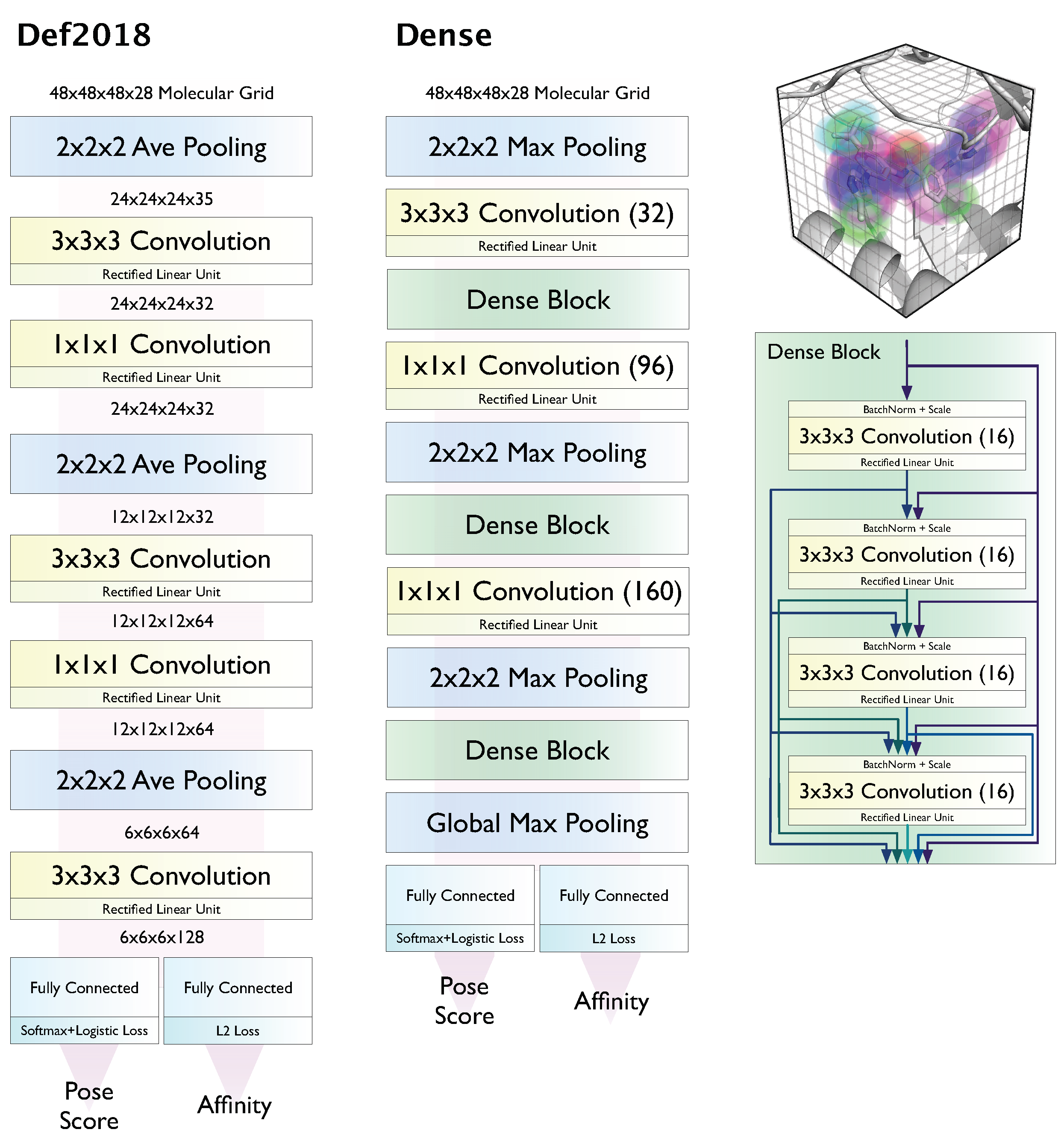
2.1. Models
2.2. Metrics
2.3. Benchmarks
2.4. Comparisons
3. Results
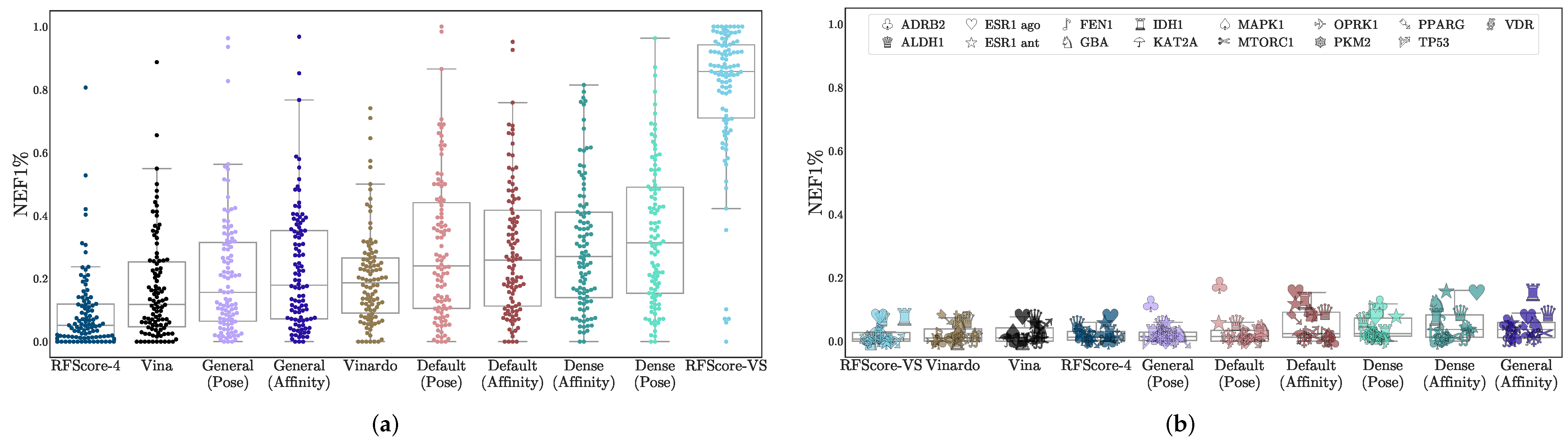
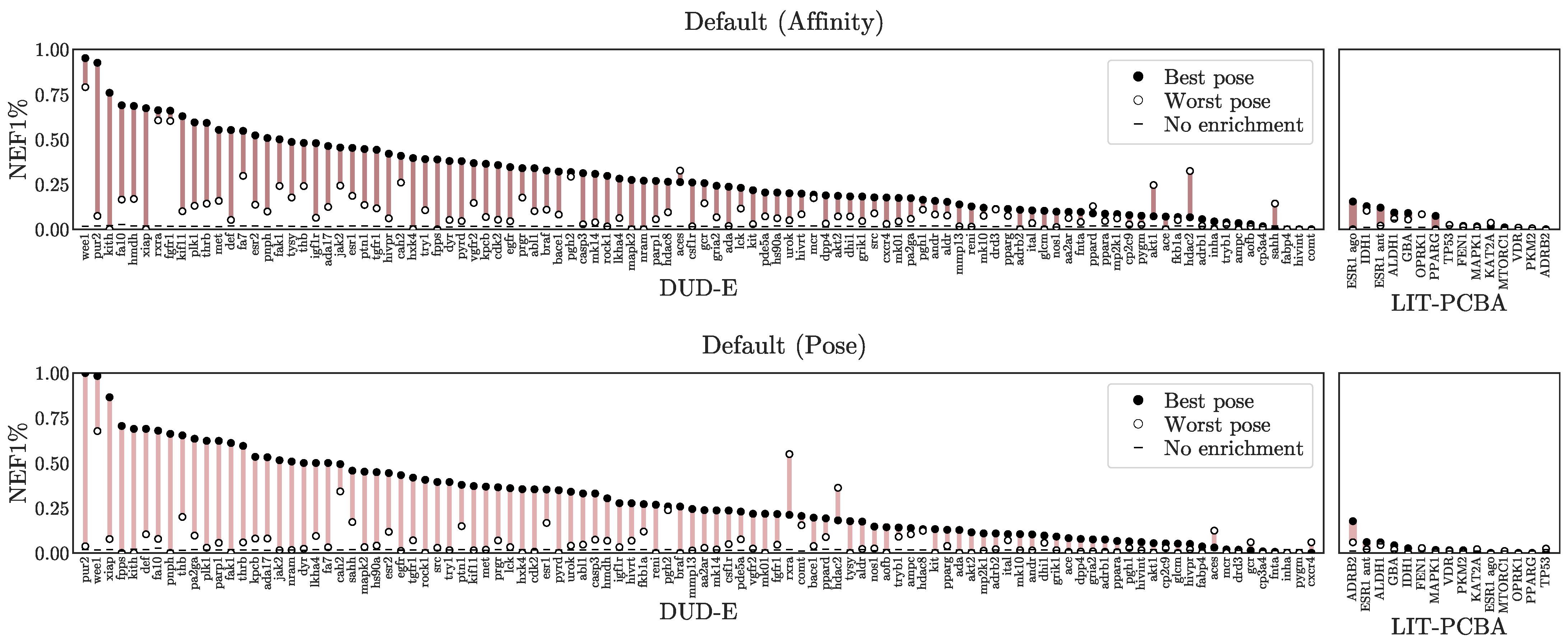
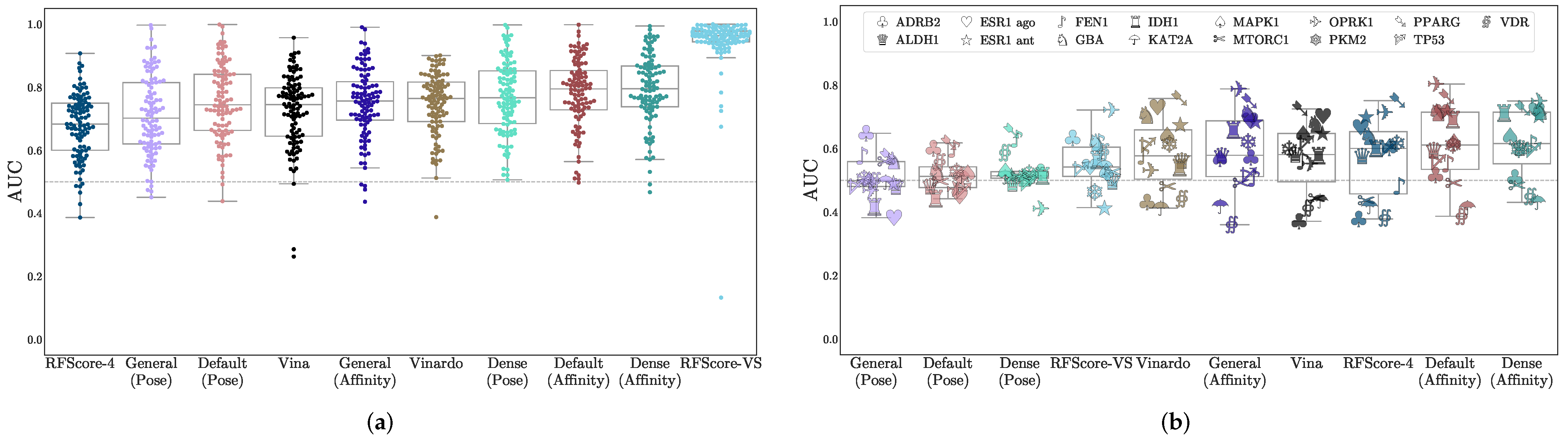
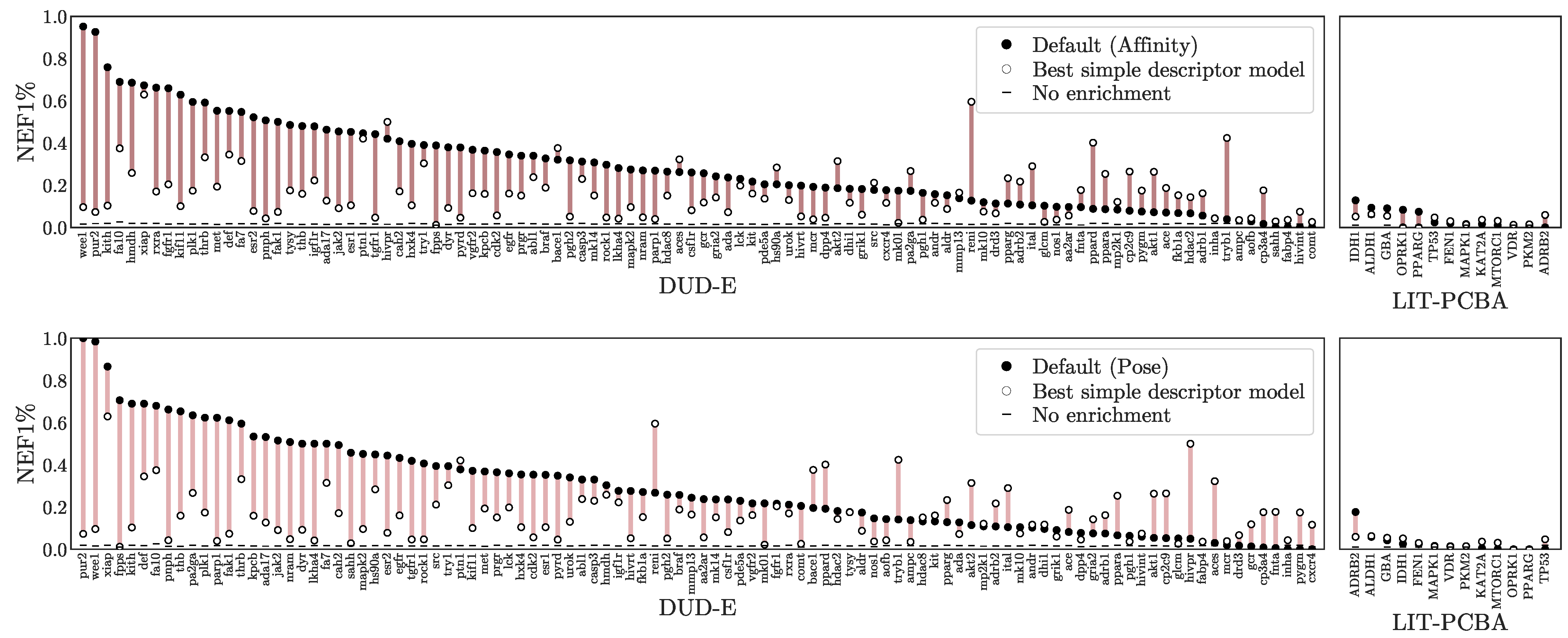
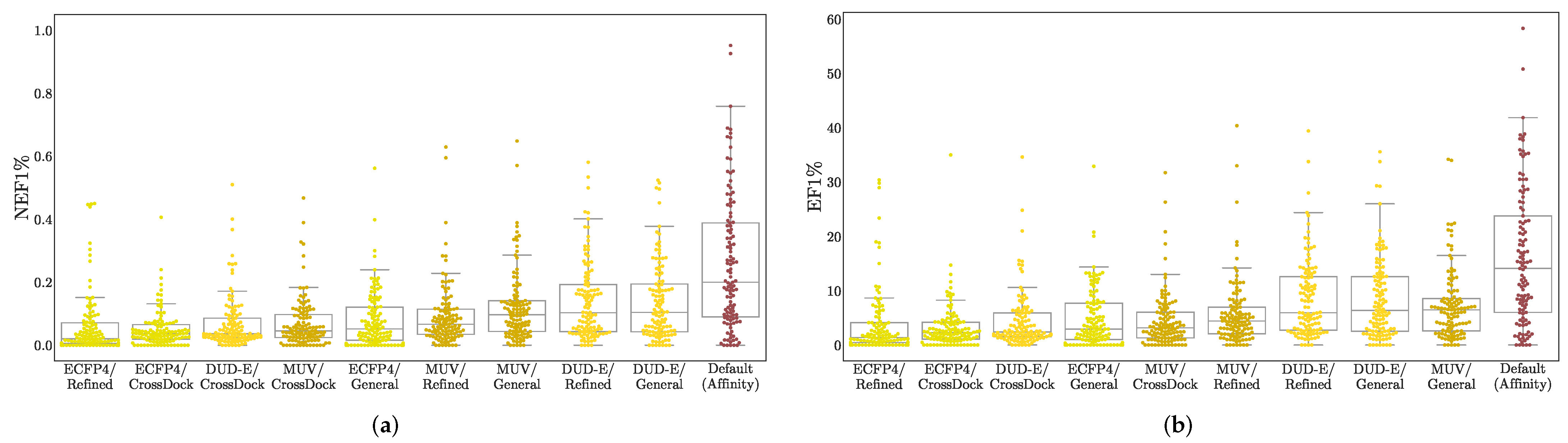
3.1. Virtual Screening Performance
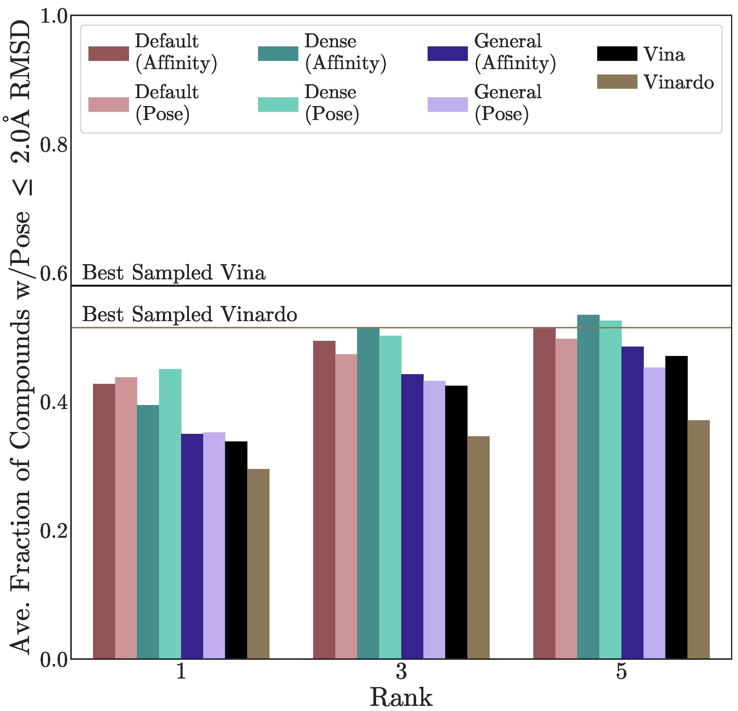
3.2. Pose Prediction Performance
3.3. Understanding Performance
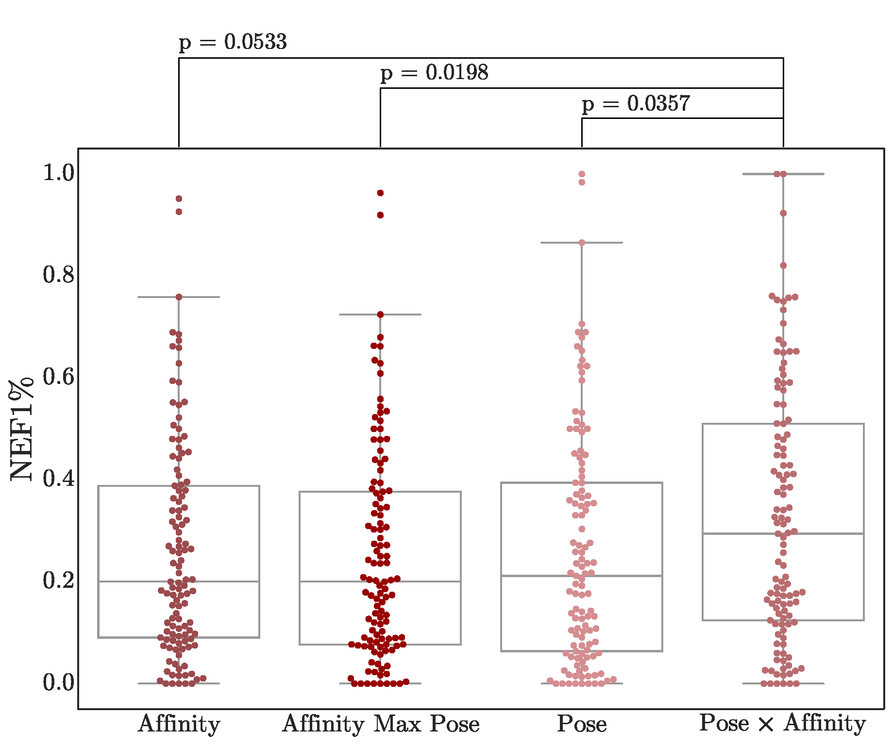
3.4. Score Adjustment
4. Conclusions
Supplementary Materials
Author Contributions
Funding
Institutional Review Board Statement
Informed Consent Statement
Data Availability Statement
Conflicts of Interest
Sample Availability
References
- Huang, S.Y.; Grinter, S.Z.; Zou, X. Scoring functions and their evaluation methods for protein–ligand docking: Recent advances and future directions. Phys. Chem. Chem. Phys. 2010, 12, 12899–12908. [Google Scholar] [CrossRef]
- Harder, E.; Damm, W.; Maple, J.; Wu, C.; Reboul, M.; Xiang, J.Y.; Wang, L.; Lupyan, D.; Dahlgren, M.K.; Knight, J.L.; et al. OPLS3: A Force Field Providing Broad Coverage of Drug-like Small Molecules and Proteins. J. Chem. Theory Comput. 2016, 12, 281–296. [Google Scholar] [CrossRef] [PubMed]
- Yin, S.; Biedermannova, L.; Vondrasek, J.; Dokholyan, N.V. MedusaScore: An Accurate Force Field-Based Scoring Function for Virtual Drug Screening. J. Chem. Inf. Model. 2008, 48, 1656–1662. [Google Scholar] [CrossRef] [PubMed] [Green Version]
- Case, D.A.; Cheatham, T.E.; Darden, T.; Gohlke, H.; Luo, R.; Merz, K.M.; Onufriev, A.; Simmerling, C.; Wang, B.; Woods, R.J. The Amber biomolecular simulation programs. J. Comput. Chem. 2005, 26, 1668–1688. [Google Scholar] [CrossRef] [PubMed] [Green Version]
- Cheng, T.; Li, X.; Li, Y.; Liu, Z.; Wang, R. Comparative assessment of scoring functions on a diverse test set. J. Chem. Inf. Model. 2009, 49, 1079–1093. [Google Scholar] [CrossRef] [PubMed]
- Ewing, T.J.; Makino, S.; Skillman, A.G.; Kuntz, I.D. DOCK 4.0: Search strategies for automated molecular docking of flexible molecule databases. J. Comput. Aided Mol. Des. 2001, 15, 411–428. [Google Scholar] [CrossRef]
- Brooks, B.R.; Bruccoleri, R.E.; Olafson, B.D. CHARMM: A program for macromolecular energy, minimization, and dynamics calculations. J. Comput. Chem. 1983, 4, 187–217. [Google Scholar] [CrossRef]
- Lindahl, E.; Hess, B.; Van Der Spoel, D. GROMACS 3.0: A package for molecular simulation and trajectory analysis. J. Mol. Model. 2001, 7, 306–317. [Google Scholar] [CrossRef]
- Jorgensen, W.L.; Maxwell, D.S.; Tirado-Rives, J. Development and testing of the OPLS all-atom force field on conformational energetics and properties of organic liquids. J. Am. Chem. Soc. 1996, 118, 11225–11236. [Google Scholar] [CrossRef]
- Jones, G.; Willett, P.; Glen, R.C.; Leach, A.R.; Taylor, R. Development and validation of a genetic algorithm for flexible docking. J. Mol. Biol. 1997, 267, 727–748. [Google Scholar] [CrossRef] [Green Version]
- Koes, D.R.; Baumgartner, M.P.; Camacho, C.J. Lessons learned in empirical scoring with smina from the CSAR 2011 benchmarking exercise. J. Chem. Inf. Model. 2013, 53, 1893–1904. [Google Scholar] [CrossRef] [PubMed]
- Eldridge, M.D.; Murray, C.W.; Auton, T.R.; Paolini, G.V.; Mee, R.P. Empirical scoring functions: I. The development of a fast empirical scoring function to estimate the binding affinity of ligands in receptor complexes. J. Comput. Aided Mol. Des. 1997, 11, 425–445. [Google Scholar] [CrossRef]
- Böhm, H.J. The development of a simple empirical scoring function to estimate the binding constant for a protein-ligand complex of known three-dimensional structure. J. Comput. Aided Mol. Des. 1994, 8, 243–256. [Google Scholar] [CrossRef] [PubMed]
- Wang, R.; Lai, L.; Wang, S. Further development and validation of empirical scoring functions for structure-based binding affinity prediction. J. Comput. Aided Mol. Des. 2002, 16, 11–26. [Google Scholar] [CrossRef]
- Korb, O.; Stützle, T.; Exner, T.E. Empirical scoring functions for advanced protein-ligand docking with PLANTS. J. Chem. Inf. Model. 2009, 49, 84–96. [Google Scholar] [CrossRef] [PubMed]
- Friesner, R.A.; Banks, J.L.; Murphy, R.B.; Halgren, T.A.; Klicic, J.J.; Mainz, D.T.; Repasky, M.P.; Knoll, E.H.; Shelley, M.; Perry, J.K.; et al. Glide: A new approach for rapid, accurate docking and scoring. 1. Method and assessment of docking accuracy. J. Med. Chem. 2004, 47, 1739–1749. [Google Scholar] [CrossRef]
- Trott, O.; Olson, A.J. AutoDock Vina: Improving the speed and accuracy of docking with a new scoring function, efficient optimization, and multithreading. J. Comput. Chem. 2010, 31, 455–461. [Google Scholar] [CrossRef] [Green Version]
- Huang, S.Y.; Zou, X. Mean-Force Scoring Functions for Protein-Ligand Binding. Annu. Rep. Comp. Chem. 2010, 6, 280–296. [Google Scholar]
- Muegge, I.; Martin, Y.C. A general and fast scoring function for protein-ligand interactions: A simplified potential approach. J. Med. Chem. 1999, 42, 791–804. [Google Scholar] [CrossRef]
- Gohlke, H.; Hendlich, M.; Klebe, G. Knowledge-based scoring function to predict protein-ligand interactions. J. Mol. Biol. 2000, 295, 337–356. [Google Scholar] [CrossRef]
- Zhou, H.; Skolnick, J. GOAP: A generalized orientation-dependent, all-atom statistical potential for protein structure prediction. Biophys. J. 2011, 101, 2043–2052. [Google Scholar] [CrossRef] [PubMed] [Green Version]
- Mooij, W.T.; Verdonk, M.L. General and targeted statistical potentials for protein-ligand interactions. Proteins 2005, 61, 272–287. [Google Scholar] [CrossRef] [PubMed]
- Huang, S.Y.; Zou, X. An iterative knowledge-based scoring function to predict protein-ligand interactions: II. Validation of the scoring function. J. Comput. Chem. 2006, 27, 1876–1882. [Google Scholar] [CrossRef] [PubMed]
- Ballester, P.J.; Mitchell, J.B.O. A machine learning approach to predicting protein-ligand binding affinity with applications to molecular docking. Bioinformatics 2010, 26, 1169–1175. [Google Scholar] [CrossRef] [Green Version]
- Li, J.; Fu, A.; Zhang, L. An overview of scoring functions used for protein–ligand interactions in molecular docking. Interdiscip. Sci. Comput. Life Sci. 2019, 11, 320–328. [Google Scholar] [CrossRef]
- Durrant, J.D.; McCammon, J.A. NNScore 2.0: A Neural-Network Receptor-Ligand Scoring Function. J. Chem. Inf. Model. 2011, 51, 2897–2903. [Google Scholar] [CrossRef]
- Hassan, M.M.; Mogollon, D.C.; Fuentes, O.; Sirimulla, S. DLSCORE: A Deep Learning Model for Predicting Protein-Ligand Binding Affinities. ChemRxiv 2018. [Google Scholar] [CrossRef]
- Wojcikowski, M.; Kikielka, M.; Stepniwska-Dziubinska, M.M.; Siedlecki, P. Development of a protein-ligand extended connectivity (PLEC) fingerprint and its application for binding affinity predictions. Bioinformatics 2019, 35, 1334–1341. [Google Scholar] [CrossRef] [Green Version]
- Shen, C.; Ding, J.; Wang, Z.; Cao, D.; Ding, X.; Hou, T. From machine learning to deep learning: Advances in scoring functions for protein–ligand docking. Wiley Interdiscip. Rev. Comput. Mol. Sci. 2020, 10, e1429. [Google Scholar] [CrossRef]
- Li, H.; Sze, K.H.; Lu, G.; Ballester, P.J. Machine-learning scoring functions for structure-based drug lead optimization. Wiley Interdiscip. Rev. Comput. Mol. Sci. 2020, 10, e1465. [Google Scholar] [CrossRef] [Green Version]
- Ragoza, M.; Hochuli, J.; Idrobo, E.; Sunseri, J.; Koes, D.R. Protein–Ligand scoring with Convolutional neural networks. J. Chem. Inf. Model. 2017, 57, 942–957. [Google Scholar] [CrossRef] [Green Version]
- Li, H.; Leung, K.S.; Wong, M.H.; Ballester, P.J. Correcting the impact of docking pose generation error on binding affinity prediction. BMC Bioinform. 2016, 17, 308. [Google Scholar] [CrossRef] [PubMed] [Green Version]
- Sieg, J.; Flachsenberg, F.; Rarey, M. In need of bias control: Evaluating chemical data for machine learning in structure-based virtual screening. J. Chem. Inf. Model. 2019, 59, 947–961. [Google Scholar] [CrossRef] [PubMed]
- Wallach, I.; Heifets, A. Most ligand-based classification benchmarks reward memorization rather than generalization. J. Chem. Inf. Model. 2018, 58, 916–932. [Google Scholar] [CrossRef]
- Chen, L.; Cruz, A.; Ramsey, S.; Dickson, C.J.; Duca, J.S.; Hornak, V.; Koes, D.R.; Kurtzman, T. Hidden bias in the DUD-E dataset leads to misleading performance of deep learning in structure-based virtual screening. PLoS ONE 2019, 14, e0220113. [Google Scholar] [CrossRef] [PubMed]
- Huang, N.; Shoichet, B.K.; Irwin, J.J. Benchmarking sets for molecular docking. J. Med. Chem. 2006, 49, 6789–6801. [Google Scholar] [CrossRef] [Green Version]
- Mysinger, M.M.; Carchia, M.; Irwin, J.J.; Shoichet, B.K. Directory of useful decoys, enhanced (DUD-E): Better ligands and decoys for better benchmarking. J. Med. Chem. 2012, 55, 6582–6594. [Google Scholar] [CrossRef]
- Rohrer, S.G.; Baumann, K. Maximum unbiased validation (MUV) data sets for virtual screening based on PubChem bioactivity data. J. Chem. Inf. Model. 2009, 49, 169–184. [Google Scholar] [CrossRef]
- Tran-Nguyen, V.K.; Jacquemard, C.; Rognan, D. LIT-PCBA: An Unbiased Data Set for Machine Learning and Virtual Screening. J. Chem. Inf. Model. 2020, 60, 4263–4273. [Google Scholar] [CrossRef]
- Marugan, J.; Dehdashti, S.; Zheng, W.; Southall, N.; Inglese, J.; Austin, C. HTS for Identification of Inhibitors against the ERK Signaling Pathway Using a Homogenous Cell-Based Assay; Probe Reports from the NIH Molecular Libraries Program [Internet]; National Center for Biotechnology Information: Bethesa, MD, USA, 2010. [Google Scholar]
- McNutt, A.T.; Francoeur, P.; Aggarwal, R.; Masuda, T.; Meli, R.; Ragoza, M.; Sunseri, J.; Koes, D.R. GNINA 1.0: Molecular docking with deep learning. J. Cheminform. 2021, 13, 43. [Google Scholar] [CrossRef]
- Ragoza, M.; Turner, L.; Koes, D.R. Ligand pose optimization with atomic grid-based convolutional neural networks. arXiv 2017, arXiv:1710.07400. [Google Scholar]
- Sunseri, J.; King, J.E.; Francoeur, P.G.; Koes, D.R. Convolutional neural network scoring and minimization in the D3R 2017 community challenge. J. Comput. Aided Mol. Des. 2019, 33, 19–34. [Google Scholar] [CrossRef]
- Hochuli, J.; Helbling, A.; Skaist, T.; Ragoza, M.; Koes, D.R. Visualizing convolutional neural network protein-ligand scoring. J. Mol. Graph. Model. 2018, 84, 96–108. [Google Scholar] [CrossRef]
- Francoeur, P.G.; Masuda, T.; Sunseri, J.; Jia, A.; Iovanisci, R.B.; Snyder, I.; Koes, D.R. Three-dimensional convolutional neural networks and a cross-docked data set for structure-based drug design. J. Chem. Inf. Model. 2020, 60, 4200–4215. [Google Scholar] [CrossRef]
- Sunseri, J.; Ragoza, M.; Collins, J.; Koes, D.R. A D3R prospective evaluation of machine learning for protein-ligand scoring. J. Comput. Aided Mol. Des. 2016, 30, 761–771. [Google Scholar] [CrossRef] [PubMed] [Green Version]
- Li, J.; Liu, W.; Song, Y.; Xia, J. Improved method of structure-based virtual screening based on ensemble learning. RSC Adv. 2020, 10, 7609–7618. [Google Scholar] [CrossRef]
- Norinder, U.; Carlsson, L.; Boyer, S.; Eklund, M. Introducing conformal prediction in predictive modeling. A transparent and flexible alternative to applicability domain determination. J. Chem. Inf. Model. 2014, 54, 1596–1603. [Google Scholar] [CrossRef] [PubMed]
- Cortés-Ciriano, I.; Bender, A. Deep confidence: A computationally efficient framework for calculating reliable prediction errors for deep neural networks. J. Chem. Inf. Model. 2018, 59, 1269–1281. [Google Scholar] [CrossRef] [Green Version]
- Liu, S.; Alnammi, M.; Ericksen, S.S.; Voter, A.F.; Ananiev, G.E.; Keck, J.L.; Hoffmann, F.M.; Wildman, S.A.; Gitter, A. Practical model selection for prospective virtual screening. J. Chem. Inf. Model. 2018, 59, 282–293. [Google Scholar] [CrossRef] [PubMed] [Green Version]
- Quiroga, R.; Villarreal, M.A. Vinardo: A scoring function based on autodock vina improves scoring, docking, and virtual screening. PLoS ONE 2016, 11, e0155183. [Google Scholar] [CrossRef] [Green Version]
- Wójcikowski, M.; Ballester, P.J.; Siedlecki, P. Performance of machine-learning scoring functions in structure-based virtual screening. Sci. Rep. 2017, 7, 46710. [Google Scholar] [CrossRef] [Green Version]
- Pedregosa, F.; Varoquaux, G.; Gramfort, A.; Michel, V.; Thirion, B.; Grisel, O.; Blondel, M.; Prettenhofer, P.; Weiss, R.; Dubourg, V.; et al. Scikit-learn: Machine Learning in Python. J. Mach. Learn. Res. 2011, 12, 2825–2830. [Google Scholar]
- O’Boyle, N.M.; Banck, M.; James, C.A.; Morley, C.; Vandermeersch, T.; Hutchison, G.R. Open Babel: An open chemical toolbox. J. Cheminform. 2011, 3, 33. [Google Scholar] [CrossRef] [Green Version]
- Liu, Z.; Li, Y.; Han, L.; Li, J.; Liu, J.; Zhao, Z.; Nie, W.; Liu, Y.; Wang, R. PDB-wide collection of binding data: Current status of the PDBbind database. Bioinformatics 2014, 31, 405–412. [Google Scholar] [CrossRef] [PubMed]
- Muchmore, S.W.; Debe, D.A.; Metz, J.T.; Brown, S.P.; Martin, Y.C.; Hajduk, P.J. Application of belief theory to similarity data fusion for use in analog searching and lead hopping. J. Chem. Inf. Model. 2008, 48, 941–948. [Google Scholar] [CrossRef]
- Ricci-Lopez, J.; Aguila, S.A.; Gilson, M.K.; Brizuela, C.A. Improving Structure-Based Virtual Screening with Ensemble Docking and Machine Learning. J. Chem. Inf. Model. 2021, 61, 5362–5376. [Google Scholar] [CrossRef]
- Shen, C.; Hu, Y.; Wang, Z.; Zhang, X.; Pang, J.; Wang, G.; Zhong, H.; Xu, L.; Cao, D.; Hou, T. Beware of the generic machine learning-based scoring functions in structure-based virtual screening. Brief. Bioinform. 2020, 22, bbaa070. [Google Scholar] [CrossRef] [PubMed]


| DUD-E | MUV |
|---|---|
| molecular weight | |
| number of hydrogen bond acceptors | number of hydrogen bond acceptors |
| number of hydrogen bond donors | number of hydrogen bond donors |
| number of rotatable bonds | |
| logP | logP |
| net charge | |
| number of all atoms | |
| number of heavy atoms | |
| number of boron atoms | |
| number of bromine atoms | |
| number of carbon atoms | |
| number of chlorine atoms | |
| number of fluorine atoms | |
| number of iodine atoms | |
| number of nitrogen atoms | |
| number of oxygen atoms | |
| number of phosphorus atoms | |
| number of sulfur atoms | |
| number of chiral centers | |
| number of ring systems | |
| 6 features | 17 features |
| Model | DUD-E | LIT-PCBA | ||||
|---|---|---|---|---|---|---|
| AUC | NEF1% | EF1% | AUC | NEF1% | EF1% | |
| RFScore-4 | 0.683 | 0.0514 | 3.02 | 0.6 | 0.013 | 1.28 |
| RFScore-VS | 0.963 | 0.857 | 51.9 | 0.542 | 0.00733 | 0.733 |
| Vina | 0.745 | 0.118 | 7.05 | 0.581 | 0.011 | 1.1 |
| Vinardo | 0.764 | 0.187 | 11.4 | 0.577 | 0.0103 | 0.99 |
| General (Affinity) | 0.756 | 0.179 | 11.6 | 0.579 | 0.037 | 2.06 |
| General (Pose) | 0.702 | 0.156 | 10.3 | 0.498 | 0.0147 | 1.3 |
| Dense (Affinity) | 0.795 | 0.27 | 17.7 | 0.616 | 0.037 | 2.58 |
| Dense (Pose) | 0.767 | 0.313 | 20.4 | 0.514 | 0.0238 | 1.81 |
| Default (Affinity) | 0.795 | 0.258 | 15.6 | 0.611 | 0.0238 | 1.88 |
| Default (Pose) | 0.744 | 0.241 | 15.8 | 0.512 | 0.0147 | 1.47 |
Publisher’s Note: MDPI stays neutral with regard to jurisdictional claims in published maps and institutional affiliations. |
© 2021 by the authors. Licensee MDPI, Basel, Switzerland. This article is an open access article distributed under the terms and conditions of the Creative Commons Attribution (CC BY) license (https://creativecommons.org/licenses/by/4.0/).
Share and Cite
Sunseri, J.; Koes, D.R. Virtual Screening with Gnina 1.0. Molecules 2021, 26, 7369. https://doi.org/10.3390/molecules26237369
Sunseri J, Koes DR. Virtual Screening with Gnina 1.0. Molecules. 2021; 26(23):7369. https://doi.org/10.3390/molecules26237369
Chicago/Turabian StyleSunseri, Jocelyn, and David Ryan Koes. 2021. "Virtual Screening with Gnina 1.0" Molecules 26, no. 23: 7369. https://doi.org/10.3390/molecules26237369
APA StyleSunseri, J., & Koes, D. R. (2021). Virtual Screening with Gnina 1.0. Molecules, 26(23), 7369. https://doi.org/10.3390/molecules26237369