
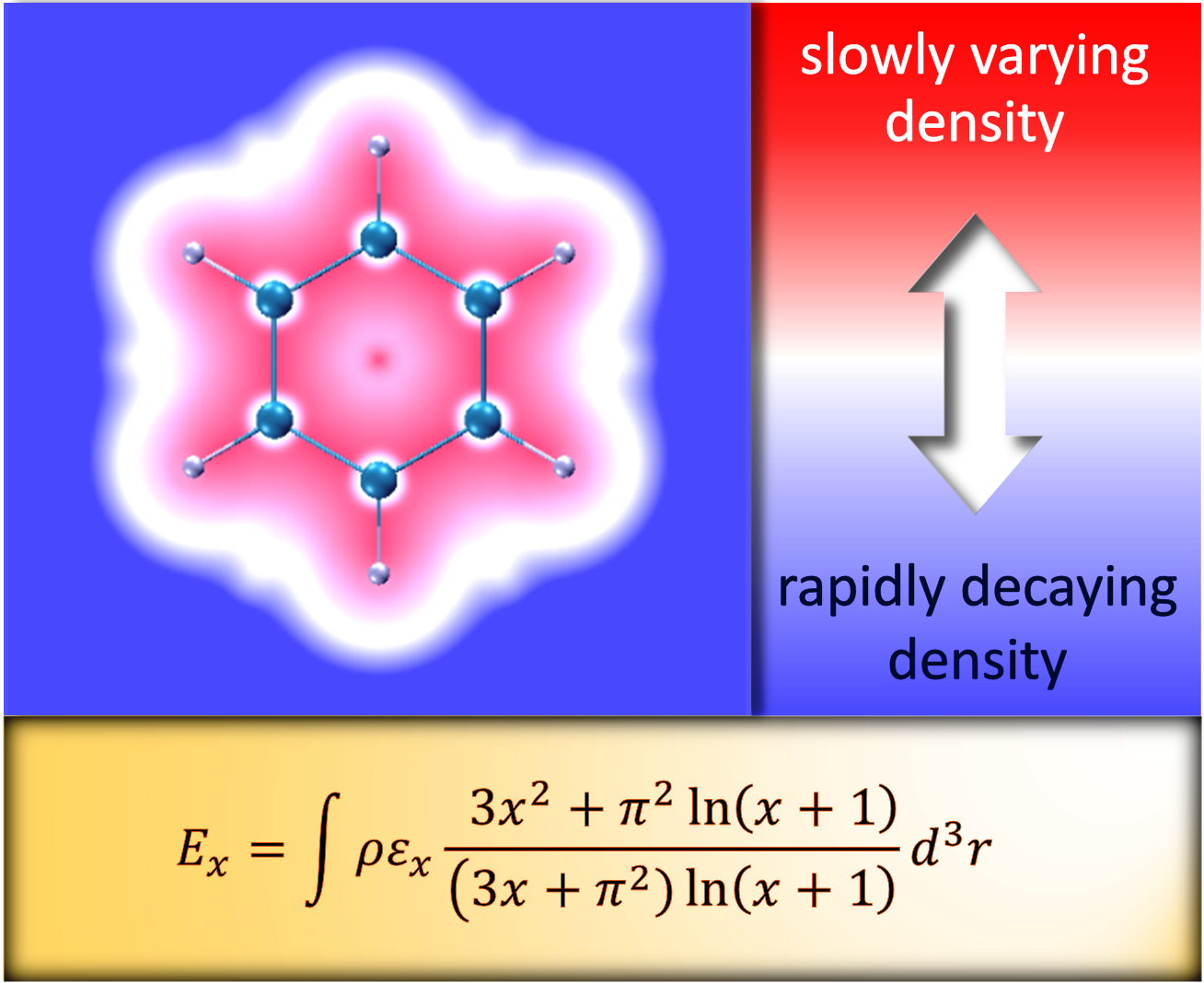
Simple and Accurate Exchange Energy for Density Functional Theory


Abstract

1. Introduction
2. Results
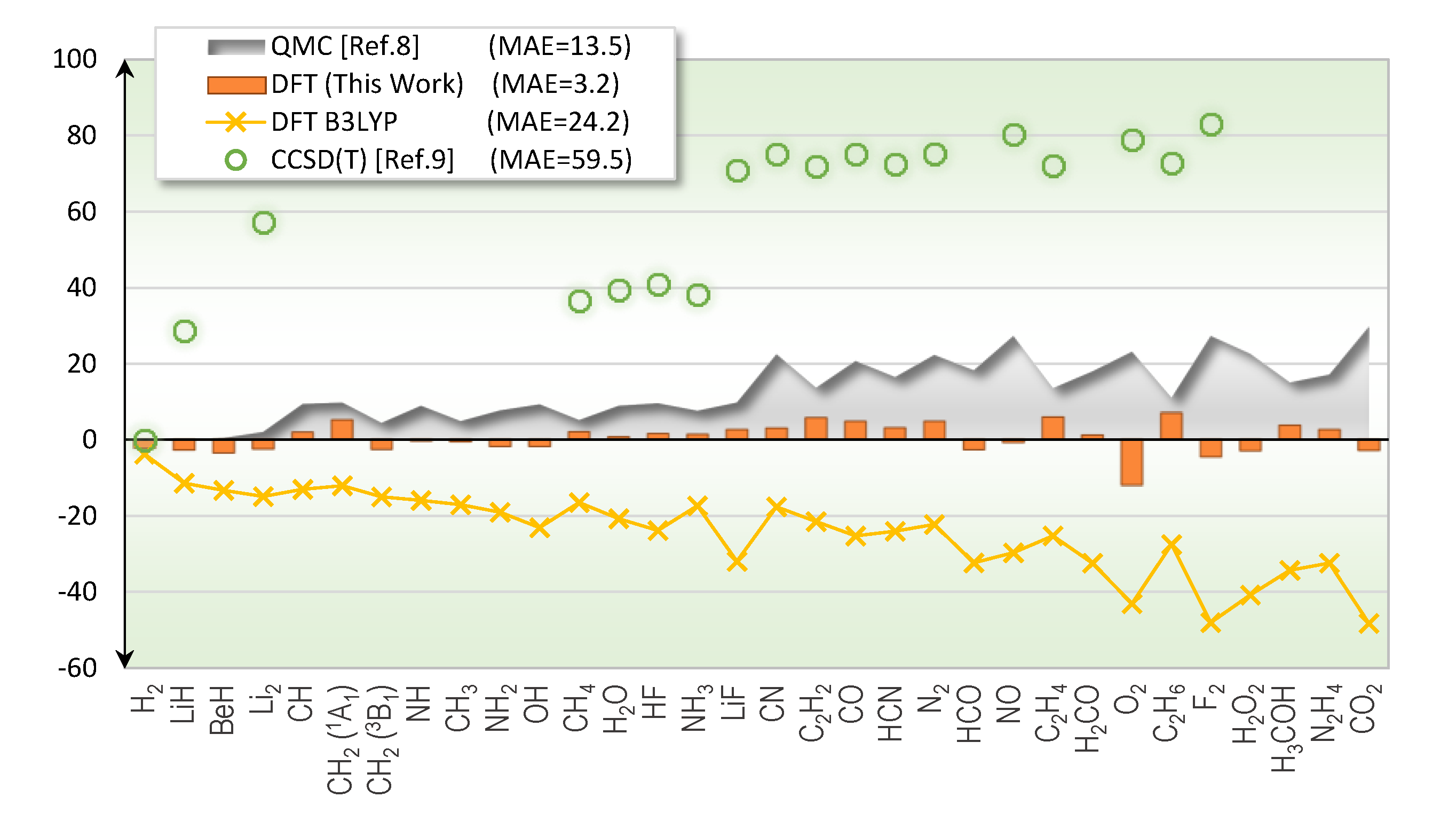
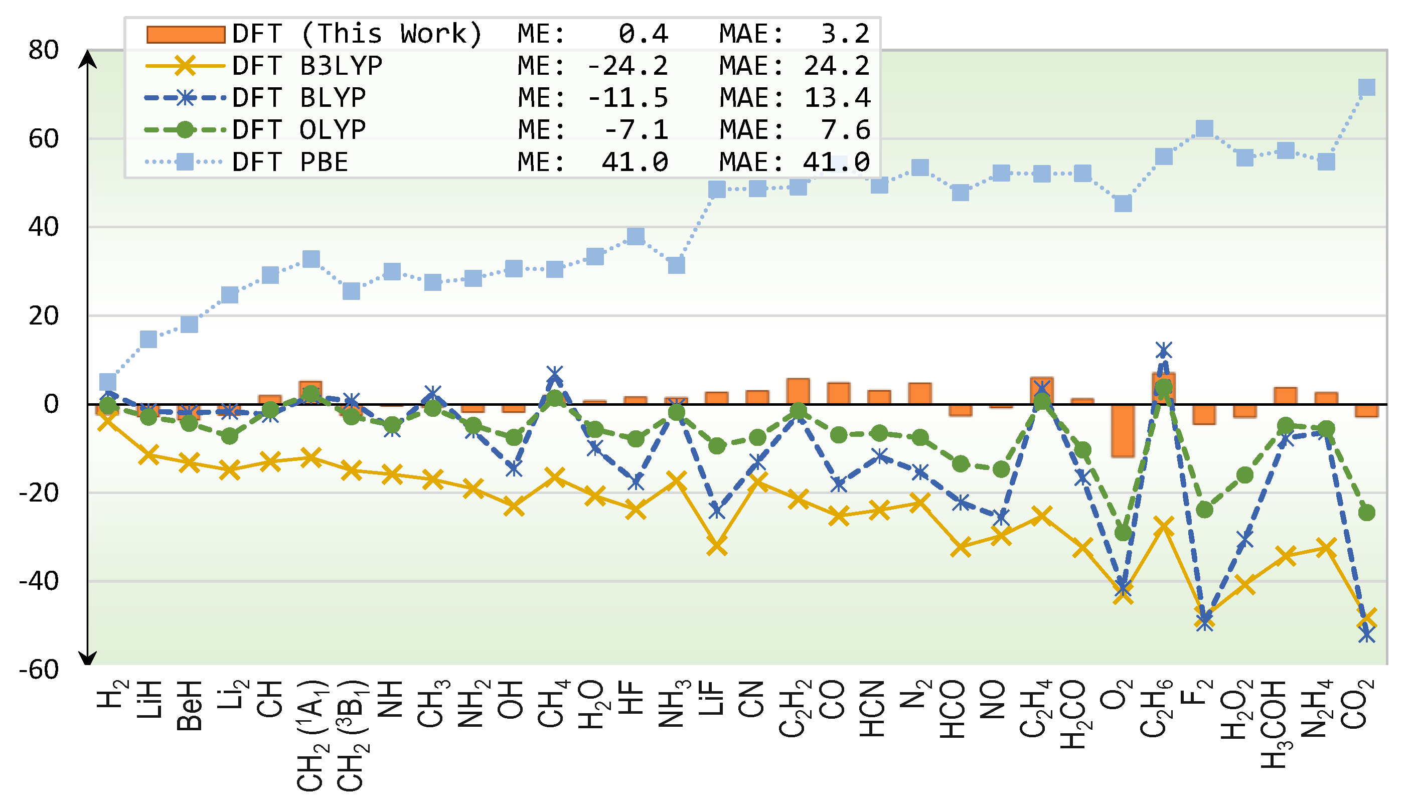
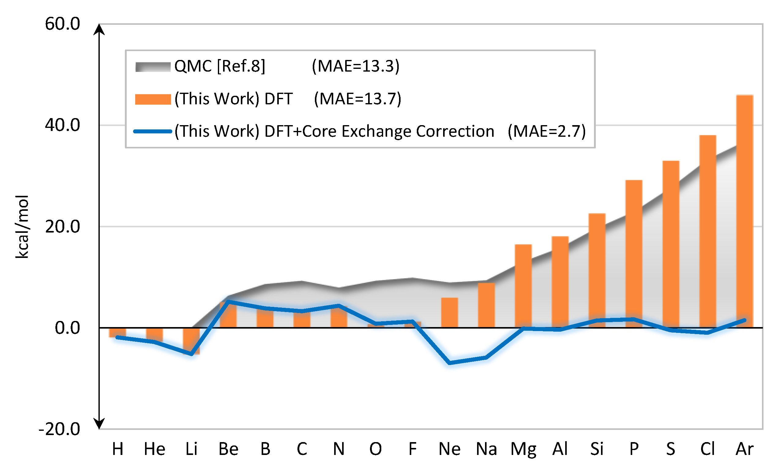
2.1. Total Energy
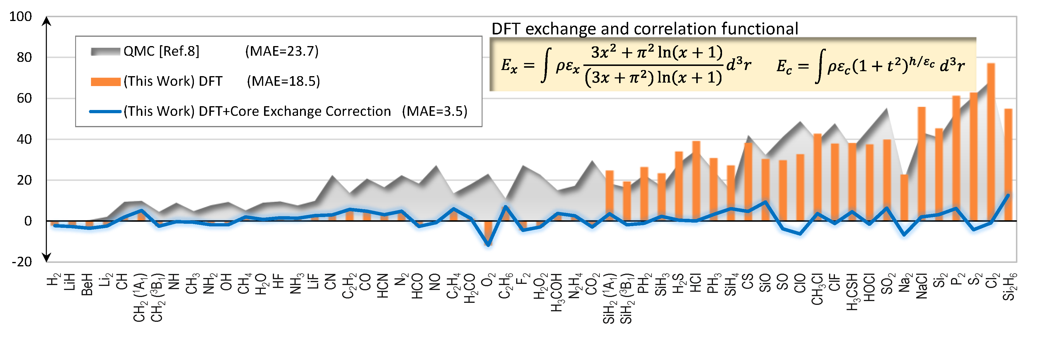
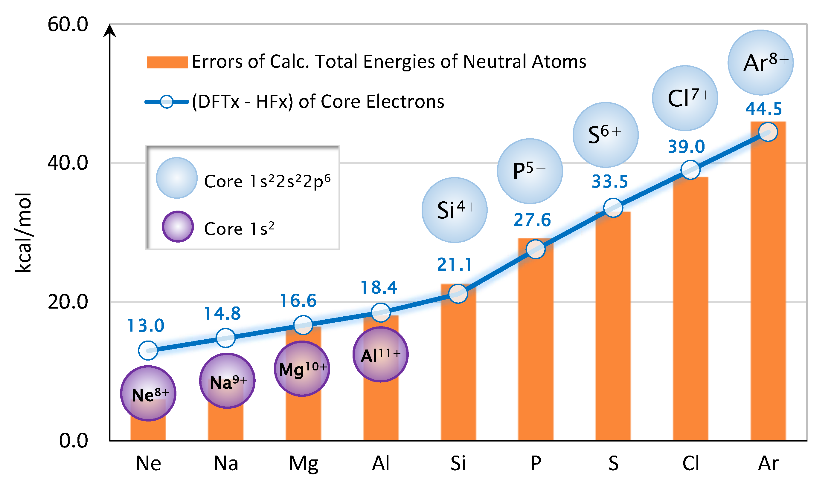
2.2. Core Exchange Correction Scheme
2.3. Bond Energy and Zero Point Energy
3. Discussion
4. Materials and Methods
5. Conclusions
Supplementary Materials
Author Contributions
Funding
Acknowledgments
Conflicts of Interest
References
- Hohenberg, P.; Kohn, W. Inhomogeneous electron gas. Phys. Rev. 1964, 136, B864–B871. [Google Scholar] [CrossRef]
- Kohn, W.; Sham, L.J. Self-consistent equations including exchange and correlation effects. Phys. Rev. 1965, 140, A1133–A1138. [Google Scholar] [CrossRef]
- Constable, E.C.; Housecroft, C.E. Chemical bonding: The journey from miniature hooks to density functional theory. Molecules 2020, 25, 2623. [Google Scholar] [CrossRef]
- Szabo, A.; Ostlund, N.S. Modern Quantum Chemistry: Introduction to Advanced Electronic Structure Theory; Dover Publications: New York, NY, USA, 1996. [Google Scholar]
- Bartlett, R.J.; Purvis, G.D. Many-body perturbation theory, coupled-pair many-electron theory, and the importance of quadruple excitations for the correlation problem. Int. J. Quantum Chem. 1978, 14, 561–581. [Google Scholar] [CrossRef]
- Needs, R.J.; Towler, M.D.; Drummond, N.D.; López Ríos, P. Continuum variational and diffusion quantum Monte Carlo calculations. J. Phys. Condens. Matter 2010, 22, 023201. [Google Scholar] [CrossRef] [PubMed]
- O’Neill, D.P.; Gill, P.M.W. Benchmark correlation energies for small molecules. Mol. Phys. 2005, 103, 763–766. [Google Scholar] [CrossRef]
- Nemec, N.; Towler, M.D.; Needs, R.J. Benchmark all-electron ab initio quantum Monte Carlo calculations for small molecules. J. Chem. Phys. 2010, 132, 034111. [Google Scholar] [CrossRef] [PubMed]
- Ranasinghe, D.S.; Petersson, G.A. CCSD(T)/CBS atomic and molecular benchmarks for H through Ar. J. Chem. Phys. 2013, 138, 144104. [Google Scholar] [CrossRef]
- Feller, D.; Peterson, K.A.; Grant Hill, J. On the effectiveness of CCSD(T) complete basis set extrapolations for atomization energies. J. Chem. Phys. 2011, 135, 044102. [Google Scholar] [CrossRef]
- Becke, A.D. Density-functional exchange-energy approximation with correct asymptotic behavior. Phys. Rev. A 1988, 38, 3098–3100. [Google Scholar] [CrossRef]
- Perdew, J.P.; Burke, K.; Ernzerhof, M. Generalized gradient approximation made simple. Phys. Rev. Lett. 1996, 77, 3865–3868. [Google Scholar] [CrossRef]
- Almbladh, C.O.; Von Barth, U. Exact results for the charge and spin densities, exchange-correlation potentials, and density-functional eigenvalues. Phys. Rev. B 1985, 31, 3231–3244. [Google Scholar] [CrossRef] [PubMed]
- Elliott, P.; Burke, K. Non-empirical derivation of the parameter in the B88 exchange functional. Can. J. Chem. 2009, 87, 1485–1491. [Google Scholar] [CrossRef]
- Kleinman, L. Exchange density-functional gradient expansion. Phys. Rev. B 1984, 30, 2223–2225. [Google Scholar] [CrossRef]
- Lehtola, S.; Steigemann, C.; Oliveira, M.J.T.; Marques, M.A.L. Recent developments in LIBXC—A comprehensive library of functionals for density functional theory. SoftwareX 2018, 7, 1–5. [Google Scholar] [CrossRef]
- Lehtola, S. Assessment of initial guesses for self-consistent field calculations. Superposition of atomic potentials: Simple yet efficient. J. Chem. Theory Comput. 2019, 15, 1593–1604. [Google Scholar] [CrossRef] [PubMed]
- Dirac, P.A.M. Note on exchange phenomena in the Thomas atom. Math. Proc. Cambridge Philos. Soc. 1930, 26, 376–385. [Google Scholar] [CrossRef]
- Chachiyo, T.; Chachiyo, H. Understanding electron correlation energy through density functional theory. Comput. Theor. Chem. 2020, 1172, 112669. [Google Scholar] [CrossRef]
- Stephens, P.J.; Devlin, F.J.; Chabalowski, C.F.; Frisch, M.J. Ab initio calculation of vibrational absorption and circular dichroism spectra using density functional force fields. J. Phys. Chem. 1994, 98, 11623–11627. [Google Scholar] [CrossRef]
- Becke, A.D. Density-functional thermochemistry. III. The role of exact exchange. J. Chem. Phys. 1993, 98, 5648–5652. [Google Scholar] [CrossRef]
- Lee, C.; Yang, W.; Parr, R.G. Development of the Colle-Salvetti correlation-energy formula into a functional of the electron density. Phys. Rev. B 1988, 37, 785–789. [Google Scholar] [CrossRef] [PubMed]
- Gill, P.M.W.; Johnson, B.G.; Pople, J.A.; Frisch, M.J. The performance of the Becke—Lee—Yang—Parr (B—LYP) density functional theory with various basis sets. Chem. Phys. Lett. 1992, 197, 499–505. [Google Scholar] [CrossRef]
- Handy, N.C.; Cohen, A.J. Left-right correlation energy. Mol. Phys. 2001, 99, 403–412. [Google Scholar] [CrossRef]
- Dale, S.G.; Johnson, E.R.; Becke, A.D. Interrogating the Becke’05 density functional for non-locality information. J. Chem. Phys. 2017, 147, 154103. [Google Scholar] [CrossRef] [PubMed]
- Jensen, F. Unifying general and segmented contracted basis sets. Segmented polarization consistent basis sets. J. Chem. Theory Comput. 2014, 10, 1074–1085. [Google Scholar] [CrossRef] [PubMed]
- Scott, A.P.; Radom, L. Harmonic vibrational frequencies: An evaluation of Hartree−Fock, Møller−Plesset, quadratic configuration interaction, density functional theory, and semiempirical scale factors. J. Phys. Chem. 1996, 100, 16502–16513. [Google Scholar] [CrossRef]
- Lide, D.R. CRC Handbook of Chemistry and Physics: A Ready-Reference of Chemical and Physical Data; CRC Press: Boca Raton, FL, USA, 2005. [Google Scholar]
- Brown, M.D.; Trail, J.R.; López Ríos, P.; Needs, R.J. Energies of the first row atoms from quantum Monte Carlo. J. Chem. Phys. 2007, 126, 224110. [Google Scholar] [CrossRef]
- March, N.H. Asymptotic formula far from nucleus for exchange energy density in Hartree-Fock theory of closed-shell atoms. Phys. Rev. A 1987, 36, 5077–5078. [Google Scholar] [CrossRef]
- Kittel, C. Introduction to Solid State Physics; John Wiley & Sons: New York, NY, USA, 1996. [Google Scholar]
- Barbieri, P.L.; Fantin, P.A.; Jorge, F.E. Gaussian basis sets of triple and quadruple zeta valence quality for correlated wave functions. Mol. Phys. 2006, 104, 2945–2954. [Google Scholar] [CrossRef]
- Schuchardt, K.L.; Didier, B.T.; Elsethagen, T.; Sun, L.; Gurumoorthi, V.; Chase, J.; Li, J.; Windus, T.L. Basis set exchange: A community database for computational sciences. J. Chem. Inf. Model. 2007, 47, 1045–1052. [Google Scholar] [CrossRef]
- A compact open-source quantum simulation software for molecules. Siam Quantum, 1.2.15; Chachiyo, T.: Phitsanulok, Thailand, 2020. [Google Scholar]
Sample Availability: Samples of the compounds are not available from the authors. |


| Equations (1) and (2) | Equations (1) and (2) | |
|---|---|---|
| Total Energy | ||
| ME | 16.9 | 1.0 |
| MAE | 18.5 | 3.5 |
| first-row ME | 0.4 | 0.4 |
| first-row MAE | 3.2 | 3.2 |
| Bond Energy | ||
| ME | −1.9 | −1.0 |
| MAE | 4.7 | 3.5 |
| first-row ME | −0.3 | −0.4 |
| first-row MAE | 4.4 | 3.2 |
| Dipole Moment | ||
| MAE | 0.11 | |
| Zero Point Energy | ||
| MAE (6–31G*) | 0.12 |
© 2020 by the authors. Licensee MDPI, Basel, Switzerland. This article is an open access article distributed under the terms and conditions of the Creative Commons Attribution (CC BY) license (http://creativecommons.org/licenses/by/4.0/).
Share and Cite
Chachiyo, T.; Chachiyo, H. Simple and Accurate Exchange Energy for Density Functional Theory. Molecules 2020, 25, 3485. https://doi.org/10.3390/molecules25153485
Chachiyo T, Chachiyo H. Simple and Accurate Exchange Energy for Density Functional Theory. Molecules. 2020; 25(15):3485. https://doi.org/10.3390/molecules25153485
Chicago/Turabian StyleChachiyo, Teepanis, and Hathaithip Chachiyo. 2020. "Simple and Accurate Exchange Energy for Density Functional Theory" Molecules 25, no. 15: 3485. https://doi.org/10.3390/molecules25153485
APA StyleChachiyo, T., & Chachiyo, H. (2020). Simple and Accurate Exchange Energy for Density Functional Theory. Molecules, 25(15), 3485. https://doi.org/10.3390/molecules25153485