1. Introduction
The Vaia storm, which occurred in Northeastern Italy at the end of October 2018, felled large volumes of timber causing serious ecological and financial losses, with unexpected challenges for forest managers. The wind gusts exceeded 200 km h
−1; over 490 Municipalities in six administrative Regions registered forest damages over an area of 67,000 km
2 [
1,
2,
3].
Windstorms are a major disturbance factor for European forests, as more than half of all the damage to forests by volume is due to wind. Since 1950, more than 130 storms have been recorded, causing notable damage to forests in Europe with on average two destructive storms each year and 38 million cubic meters of forest destroyed per year. Frequent disturbances by wind damage may alter the forest C sequestration capacity; if forest ecosystems are to be accounted for in mitigating atmospheric carbon dioxide (CO
2), it is important to quantify the impacts of disturbance [
4]. A repeated disturbance may also have an influence on biodiversity [
5,
6] and promote insects and pathogens outbreaks [
7]. There is evidence that the actual severity of storms in the wake of climatic changes may increase during the next decades and that evaluating their impact on forest resources is important for all parties that are engaged in the forest economy, ecology, and planning [
8,
9].
Remote sensing is fundamental for both primary assessment of damages and post-emergency phase, to get a more precise view of the actual damage and plan for the salvage of the wood and the restocking of the area. In general, a combination of field inventory and remote sensing approaches are needed to establish the area, the volume, the species, the quality, and the percentage of trees damaged in stands [
8]. Possibly, the most effective remote sensing data to monitor forest damages are those collected through airborne platforms, such as very high spatial resolution aerial photographs that are often used by public forest services [
10]. Lidar data showed to be useful as well, not only to delineate the damaged areas but also to provide an evaluation of the volume of fallen trees [
11,
12]. However, airborne surveys are expensive, can be conducted on a limited area, and are difficult to be carried out under adverse meteorological conditions that often persists for weeks after a storm.
Satellite remote sensing data cover large spatial extents providing repeated information at lower costs. Jointly used with ground truth collected by professional foresters, satellite data can help to both delineate the forest areas impacted by windthrow, as well as to estimate the damages.
The delineation of impacted areas is frequently carried out with optical data [
1,
2,
3,
13], even if cloud cover can delay the availability of images for months as previously evidenced also in the Vaia case [
14]. Synthetic Aperture Radar (SAR) data may also be employed, even if it requires expert knowledge. SAR data have the advantage of being weather insensitive, providing also forest structural information, and being complementary to optical data [
15,
16,
17].
The estimation of the volume of fallen trees, or above ground biomass (AGB), is a more complex task with respect to delineation of damaged areas. Optical data are of limited help due to saturation effects occurring at medium and even low AGB values [
18]. Since 2000, when SAR space-borne systems started delivering repeated data, many studies have exploited SAR data for above-ground biomass estimation [
19,
20]. In the case of windthrown, knowing the amount of AGB occurring in a forest prior to the event allows for an estimation of the fallen timber amount after the impact.
The explicit estimation of the timber loss caused by Vaia using satellite remote sensing was not yet undertaken, and here it was attempted for the first time. [
21] attempted the prediction of damage severity in a test area, using a combination of remote sensing, machine learning, and Web-GIS tools, based on Sentinel 2 vegetation indices. [
22] summarized data on impacts provided by local administrations, aggregated at municipality level. [
23] highlighted the inconsistencies of data on Vaia damages delivered by local administrations, both among them and with respect to national level data. Unfortunately, there was a delay in publishing the 3rd (2015) national forest inventory results, causing a lack of recent data on forest stocks and fluxes, and no information is availableto establish the amount of fallen timber prior to the event. Furthermore, the Italian National Statistics Institute (ISTAT) forest production data for 2018 did not provide statistical evidence about the Vaia catastrophic event.
The novelty of this research is in the comparison of different estimates of the timber loss caused by the Vaia event in two study sites, named Trento and UMA (Unione Montana Agordina), where Vaia caused notable damages and where only the delineation of the damaged areas was made available by official sources. The volume or biomass datasets used to quantify the amount of timber occurring pre-Vaia event were produced with different methodologies and are characterized by different accuracies. The datasets, here illustrated and compared for the first time, resemble the type of information that a forest manager might potentially find or produce, and that should be used to assist in the decision-making process. The datasets include: (a) pre-existing local growing stock volume maps based on lidar data; (b) a recent national-level volume map produced in the framework of the AgriDigit project (
www.progettoagridigit.it. Last access on: 3 November 2021) according to the methodology described in [
24]; and (c) a new AGB estimate just produced specifically for this research. Three specific objectives were defined: (i) to test a methodology for producing updated AGB information based on satellite remote sensing data temporarily close to the windthrow; (ii) to evaluate the differences in forest timber losses according to the various datasets; and (iii) to discuss the options available to properly inform forest management.
2. Materials and Methods
2.1. Study Areas and Field Data
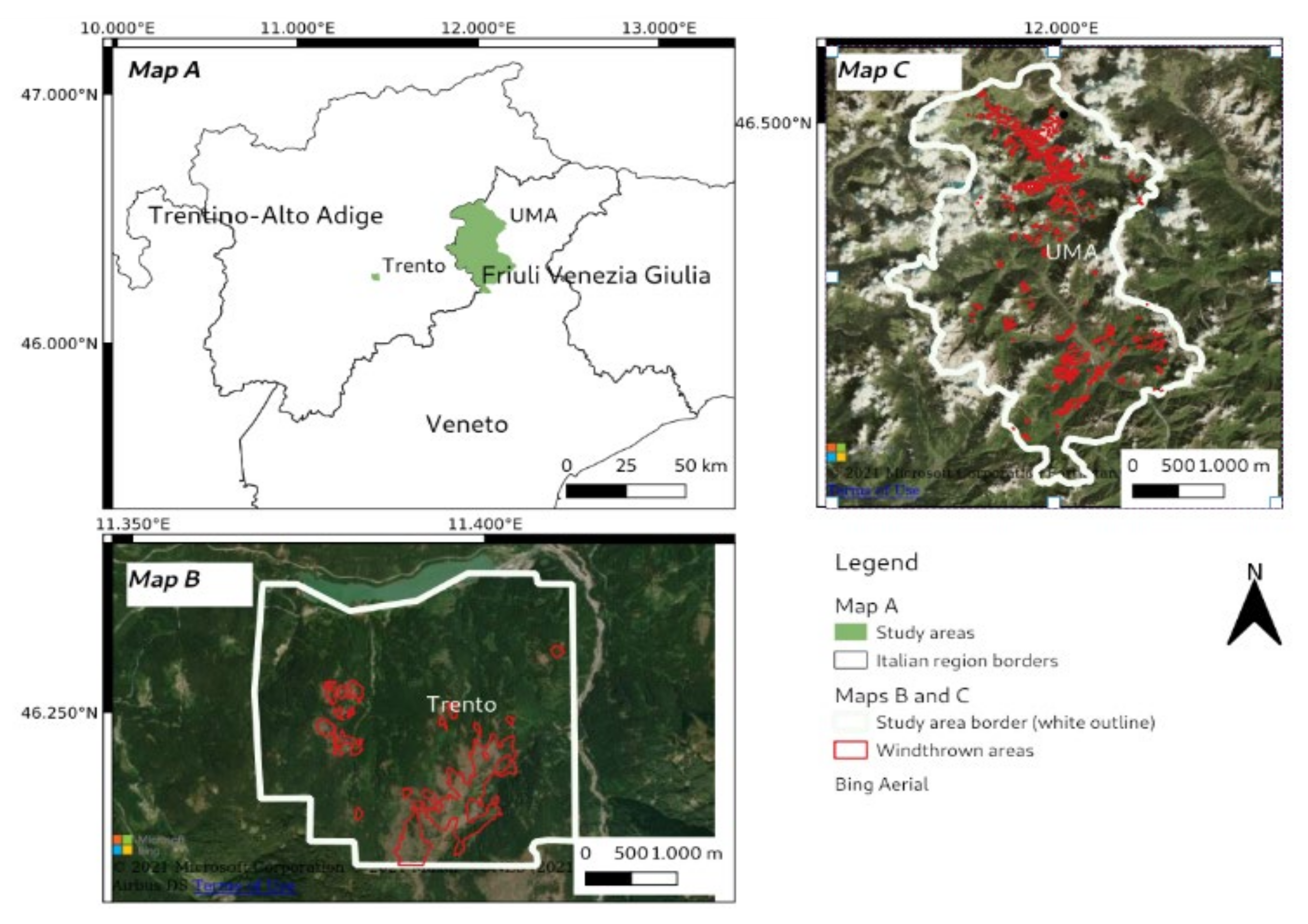
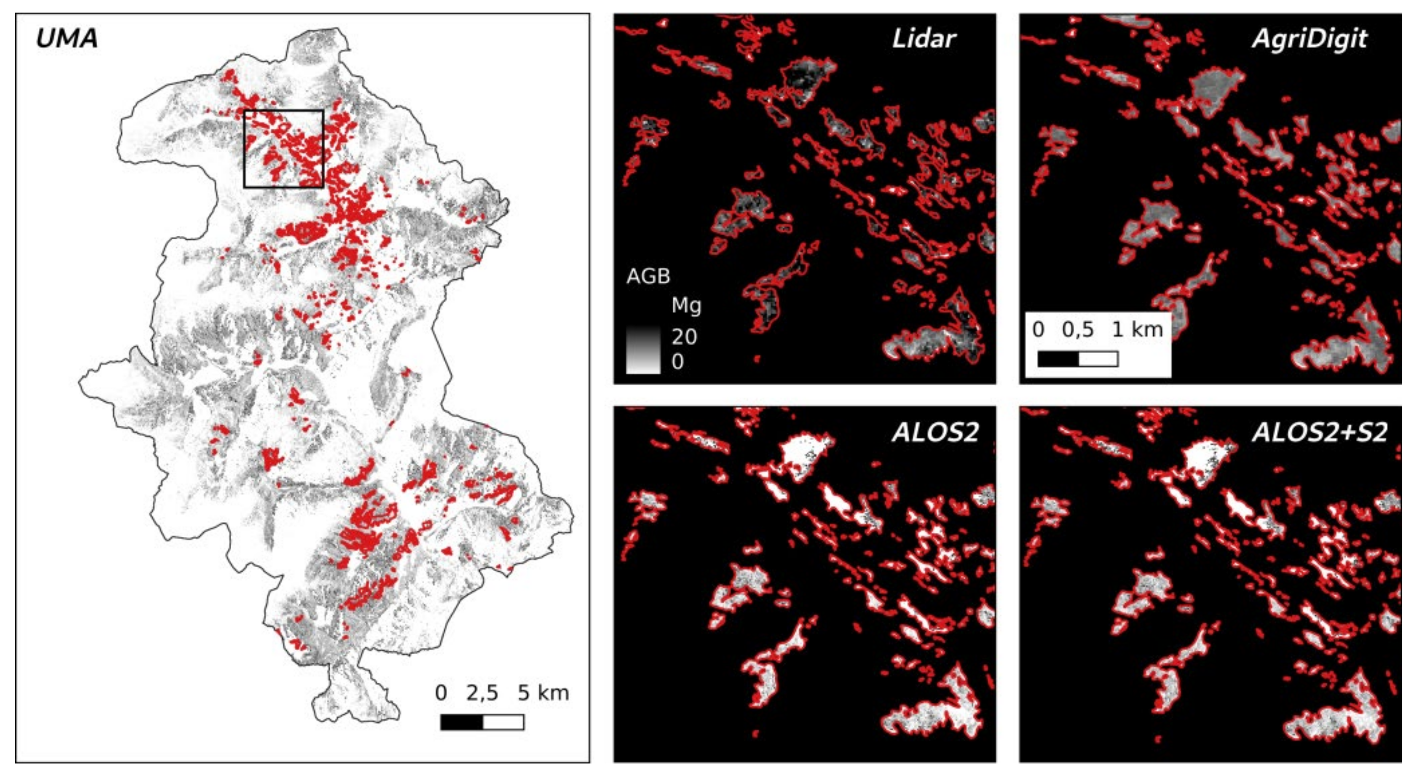
The study areas selected for this study—Trento and UMA—are both in the European Alpine Space, in a mountain range located respectively in the Trentino Alto-Adige and Veneto regions, in northern Italy (
Figure 1). The forests in this range are mainly composed of conifer species, with dominance of Picea abies and occurrence of Larix decidua, Abies alba, and Acer pseudoplatanus; deciduous stands are less diffuse and often dominated by Fagus sylvatica, also intermixed with conifer species. The two areas overlap an ALOS2 SAR Fine Beam Mode dual polarization image, that covers approximately an area of 70 × 70 km. The areas were impacted by the 2018 October Vaia storm. According to Corine Land Cover information, the Trento area is smaller, with about 1170 ha of forests, while the UMA area is larger, with about 12,340 ha of forests.
In the Trento and UMA areas, 82 ground sample plots were collected in 2018 and 2019. The height, breast height diameter (DBH), species, and the stem position of single trees with DBH values above 7.5 cm were recorded for each sample. The Trento ground dataset includes 30 plots of 15 m radius each, while UMA comprises 52 plots ranging between 13 m to 20 m radius. All samples are in the Alpine region, with an average height above sea level of 1422 m and, higher and lower heights above sea level of 2012 m and 852 m, respectively. Trento plots were sampled during the 2019 campaign [
25], while UMA was sampled in 2018 right before the Vaia event. To compute AGB plot values from DBH, species, and height information, the [
26] formulas were used. Single tree AGB values were averaged at plot level and the AGB values per plot (in Mg/ha) were obtained after normalization for plot area. Overall, the AGB collected in these 82 sample areas ranged from 6.9 to 817 Mg/ha, with average and standard deviation values of 247 Mg/ha and 142 Mg/ha, respectively.
During the modeling step, about 50% of the field plots were removed from the analysis, as they occur in steep mountain areas of SAR data distortion. Other plots were also excluded, including outliers in AGB or ALOS2 HH and HV distributions (four plots) and few plots covered by less than 3 ALOS2 pixels (a pixel was considered valid when >70% of its surface falls inside the plot). In total, 34 plots remained available for training and testing the AGB models (
Figure 2). These 34 field plots were still representative, covering a broad AGB range (6.9–619.2 Mg ha
−1), with a mean value of 218.5 Mg/ha and standard deviation of 168.8 Mg/ha. The tree species dominance occurring in these plots resulted comparable with the dominance usually reported in this Alpine mountain range, with the prevalence of Picea abies (27 plots), followed by Larix decidua (5 plots), Fagus sylvatica (1 plot), and Acer pseudoplatanus (1 plot).
2.2. Pre-Existing Volume Maps
In the Trento area, a timber volume map was generated through a single tree segmentation procedure based on an airborne lidar survey conducted in 2014 by the Autonomous Province of Trento with an OPTECH ALTM 3100 sensor, which returned a point cloud with a minimal point density of 8 points/m
2. The data were used to detect single trees with calibrated parameters according to vertical structure and chronological class. This procedure uses an adaptive distance threshold that affects the precision of tree detection, allowing for the limitation of over- and under-estimation [
25]. The tree heights and positions were extracted by segmenting the trees from the point cloud using the method defined in [
27]. The map, with 10 m spatial resolution, was validated using the Trento plots described in 2.1 and was characterized by a relative root mean squared error (RMSE) of 9.5% [
28].
In the UMA area, a timber volume map was generated by the InForTrac project (
https://infortrac.wordpress.com/. Last access on 3 November 2021) using the lidar-assisted area-based method detailed in [
29]. The input information for this method consists of a canopy height model (CHM) calculated from lidar-derived digital terrain and surface models. These models, with 1 m spatial resolution, were derived from an airborne survey of the Veneto Region carried out in 2015. The final volume map, with 25 m spatial resolution, was validated using UMA plots and has a relative RMSE equal to 8.2% [
30].
The growing stock volume map obtained within the AgriDigit project (AD23m), with a spatial resolution of 23 m, is based on different inputs including satellite data, the 2005 Italian National Forest Inventory data aggregated at 1 km grid, and auxiliary variables such as the 1981–2010 climate data gridded at 1 km spatial resolution, the European Space Agency ecoregions map, and a 2007 Digital Terrain Model. From the AgriDigit map, volume data for Trento and UMA areas were extracted; this product was just released as a service for the sub-project ‘Precision Forestry’ (July 2021) and here firstly tested. Specifically, the satellite inputs include: a Landsat 7 2004–2006 cloud free composite, the 2007 ALOS Palsar Japanese Space Agency (JAXA) mosaic, and the 2019 Canopy Height Model (CHM) data from the Global Ecosystem Dynamics Investigation (GEDI) mission. The map produced by the AgriDigit project contributes to overcoming the scarcity of information on Italian forest stocks, providing a 2005 baseline. However, the reported accuracy of this map for the mixed and conifer Alpine forests is limited, with a coefficient of determination (R2) of 0.35 and a RMSE of 67% (AgriDigit service report).
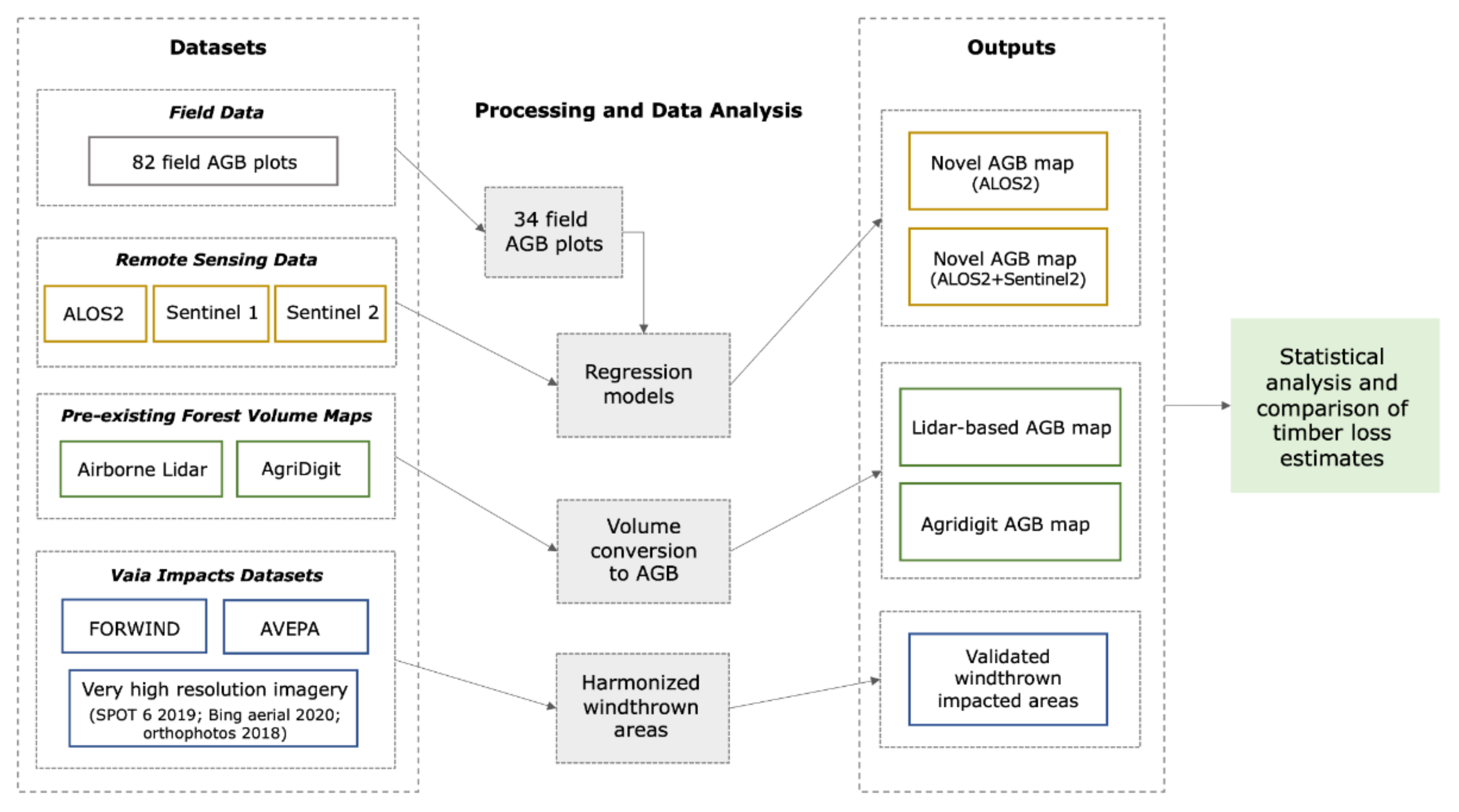
To allow comparison with the newly SAR-based biomass map generated by this research, all the volume values of the mentioned maps were converted to above ground biomass (
Figure 2). Biomass can be calculated from Volume (V) by first estimating the wood density (WD) of the volume and then “expanding” this value with a biomass expansion factor (BEF) to consider the biomass of the other aboveground components. The following [
30] formula was applied, using a WD value of 0.4 [
31] and a BEF of 1.2 [
32]:
2.3. Remote Sensing Data
To estimate the AGB occurring in the study areas right before the Vaia event, different combinations of ALOS2 (Advanced Land Observing Satellite-2), Copernicus Sentinel 1 and Sentinel 2 remote sensing data were tested.
ALOS2 is a Japanese satellite equipped with a L-band Synthetic Aperture Radar (SAR) [
33]. A Fine Beam Mode (Single Look Complex) scene covering the study areas, with dual polarization (HH and HV), from the closest date prior to the Vaia event (18 September 2018) was processed using the European Space Agency (ESA) Sentinel Application Platform (SNAP). The pre-processing included calibration, selection of Gamma naught for the analysis, speckle filtering with 3 × 3 Frost filter [
34], SAR simulation to produce the distortions mask, and Range Doppler terrain correction using the Shuttle Radar Topography Mission Digital Elevation Model at 1 Arcsec. The processed scene had a final spatial resolution of 14.5 m; areas with SAR distortions (layover, shadow, and foreshortening effects) were masked out prior to further analysis. The ALOS2 decibel values were linearized, and plot-level statistics were extracted from the two polarizations, including: minimum, maximum, mean, polarization subtraction (HH − HV), and polarization addition (HH + HV). Sentinel 1 polarizations and Sentinel 2 vegetation indices were also joined to ALOS2 data, after resampling their resolution to meet the ALOS2 one (14.5 m).
The ESA Sentinel 1 is a constellation of SAR satellites operating at C-band [
35]. An Interferometric Wide Swath SLC scene with dual polarization (VV and VH) from satellite 1B, dated 4 September 2018, was selected and processed with SNAP. The pre-processing steps included Tops Split, Slice Assembly, application of orbit file, Calibration, and selection of Gamma naught for the analysis, Tops Deburst, Tops Merge, speckle filtering with Frost 7 × 7, Multilooking 4 × 1, SAR simulation to produce the distortions mask, and Range Doppler terrain correction using the Shuttle Radar Topography Mission Digital Elevation Model at 1 Arcsec. The processed scene has a pixel spacing of 14 m; areas of SAR distortions (layover, shadow, and forthshortening effects) were masked out prior to further analysis.
The ESA Sentinel 2 is a constellation of multispectral satellites with 13 bands with 10–60 m spatial resolution. Given the lack of cloud-free images in the months prior to the Vaia event, a mosaic of cloud-free images (cloudy pixels <3%) extracted from Google Earth Engine (GEE) was generated over the study areas using images collected in the June-October months from 2015 to 2018. The mosaic was composed using pixels with the lowest cloud coverage value among those available from different dates of the time series, without using the ‘reducer’ functions available in GEE. In fact, the use of GEE reducers was discarded since it produces a mixture of spectral signatures from different images, applying an aggregation function (e.g., quantiles, average, minimum) to the vector composed by the pixels from different time series dates.
After resampling the 20 m bands at 10 m spatial resolution, 21 spectral vegetation indices were calculated, including those most frequently computed for Landsat and Sentinel 2 data [
36]. Pixels representing outliers in vegetation indices, caused by the merging of different S2 images, were excluded. The list of indices is presented in
Supplementary Materials Table S1, as well as the formulas and references. Finally, a GNDVI value >0.5 derived from Sentinel 2 composite was used to mask out non-forest areas in all the remote sensing datasets.
2.4. The Vaia Impacts Dataset
To compare the estimates of fallen timber according to different datasets, a clean layer of impacted sites for the two study areas was needed for the extraction of information. The windthrown impacted areas dataset documented by [
37] and the 2019 dataset provided by the Veneto Region agency for agriculture subsidies AVEPA (Agenzia Veneta per i Pagamenti in Agricoltura) were thus harmonized, refined, and jointly used to create a cleaned Vaia impacts dataset.
Ref. [
37] is an open access spatially explicit database of wind-related impacts at a pan-European scale for the period 2000–2018 (FORWIND). The methods used to produce this dataset include a correlation analysis between FORWIND data and land cover changes retrieved from the Landsat-based Global Forest Change dataset and the MODIS Global Disturbance Index.
The Veneto Region AVEPA dataset provides Vaia impacted areas obtained through a semi-automatic classification approach of remote sensing data (Sentinel 2, SPOT6, and SPOT7 satellite imagery from pre- and post-event dates), validated and corrected through photointerpretation of 2018 orthophotos from AGEA (Agenzia per le Erogazioni in Agricoltura).
Through the Topology Checker tool in QGIS software, inconsistencies in topology were corrected in each dataset; the areas below 100 m2 were removed to meet the resolution of the remote sensing data and volume or AGB datasets used in this study. Where available, the percentage of fallen trees was used to exclude those impacted areas with a large presence of remaining standing trees, setting a threshold of fallen trees >80% thus retaining only areas severely damaged by the storm. Information from the two datasets was joined; all the damaged areas were visually validated to further exclude sites with damages below the 80% threshold, and to improve the polygon delineation given the multiple topological inconsistencies found in both datasets.
The result was a supervised and validated dataset of Vaia impacted sites for the two study areas, Trento and UMA, that includes only polygons larger than 100 m
2, where damages were severe (>80% of fallen trees), and where a further check was performed by means of on-screen evaluation of high-resolution imagery (SPOT 6 post-event 2019 image; Bing aerial imagery 2020; and orthophotos 2018 from the Regione Veneto) (
Figure 2).
2.5. Data Analysis
The first step was to test the production of new AGB information temporarily as close as possible to the Vaia event in the two study areas, based on recent SAR and optical satellite data. To this aim, the remote sensing images detailed in paragraph 2.3 (ALOS2, Sentinel 1, and Sentinel 2) and the field data described in 2.1 were jointly used to set up and validate different regression models, then selecting the most accurate one to estimate the AGB occurring in the impacted areas prior to Vaia, and thus the timber that fell with the event.
ALOS2 was used as the main remote sensing dataset, given the well-known L-band SAR sensitivity to above ground biomass [
17,
38]. Two different algorithms were tested for modeling AGB, always using the Leave-One-Out (LOO) cross-validation approach to account for the limited amount of ground truth [
39]. Stepwise Multilinear Regression (SMLR) represents the most basic form of linear regression analysis and thus a reference [
40]. It is an iterative algorithm adding or removing terms from a linear model based on their statistical significance in explaining the response value. The model was evaluated by means of the coefficient of correlation (R2) and the Variance Inflation Factor (VIF), which provides a measure of the overfitting that might be caused by highly correlated input variables [
41]. Partial Least Square Regression (PLSR) algorithm is similar to Principal Component Regression, and it is especially suited to deal with multicollinearity effects [
42]. It is a technique that reduces the predictors to a smaller set of uncorrelated components and performs least squares regression on these components, instead of on the original data. The model was evaluated by means of the coefficient of correlation (R2), and the PRESS statistics [
43]. The most accurate models were used to generate Trento and UMA AGB predicted values.
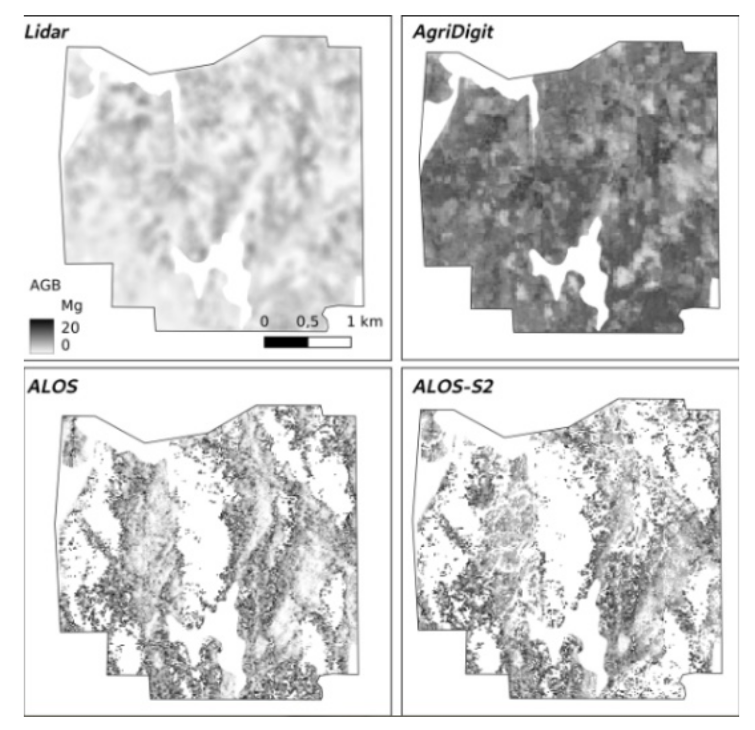
The second step was to analyze and compare the different available AGB datasets, both the pre-existing and newly produced. This step involved four different AGB datasets: the new AGB estimates based on (1) ALOS2 alone (2) ALOS2 plus Sentinel inputs; (3) the AgriDigit AGB estimates; and (4) the local lidar-based AGB estimates. First, basic statistics were computed for each dataset, masking out non forest areas according to the Corine Land Cover 2018 dataset. Then, using the Vaia impacts vector dataset defined in 2.4, the AGB values were extracted from each of the four AGB layers. An ANOVA test was firsly run to assess if there were significant differences in the results, and subsequently the Tukey’s test for multiple comparisons of means [
44] was performed, to assess which differences were significant according to each estimation method. The analysis was carried out in R [
45] (R Core Team 2021).
Figure 2 illustrates the different steps.
4. Discussion
The provision of accurate information on the amount of fallen timber after a windthrown or similar destructive event is not an easy task in the lack of spatially explicit and updated biomass or volume national data. On the other hand, this type of data is critical for making informed decisions to manage impacted forests.
Information on Vaia impacted areas was here reviewed and for the first time harmonized. The data provided by the Regione Veneto AVEPA and the EU FORWIND layer showed inconsistencies between them as well as topological issues. Hence, a refinement step based on visual interpretation of very high-resolution imagery was needed to produce a reliable layer of damaged areas. [
23] identified similar inconsistencies on Vaia windthrown data; together these evidences encourage a rapid adoption of a single methodology to map forest damages at a national level.
To quantify the fallen timber, different available layers were exploited and a novel AGB estimate was generated using ALOS2 alone or ALOS2 plus Sentinel 2 satellite data collected close to the Vaia event. Among the available layers, the preexisting lidar-based datasets can be considered a benchmark, given the high reliability of volume or biomass estimates based on laser scanning, which allows to sample the forest vertical structure at fine scale [
17,
19,
48,
49]. Even if the conversion of volume to biomass could be a potential source of error, and the coverage is partial over the UMA area (
Table 2), the Trento and UMA lidar collections are relatively recent (2014 and 2015, respectively). However, due to the high related costs, these layers are not always available and lidar data is not frequently collected. For instance, at the Italian national level the last lidar coverage was only partial, covering 43% of the country between 2008 and 2012. The option of producing volume or AGB estimates from this type of data is hampered by the lack of accessible field calibration and validation data.
The AgriDigit dataset is the most recent available estimate of forest volume for the Italian territory, and its applied use was here tested for the first time. However, the declared accuracy over the considered forest types is low, and the date and coverage of the ground samples used to train and validate the model over the study region (samples derived from 2005 Italian national forest inventory) are poor. Thus, the reliability of these estimates might be limited.
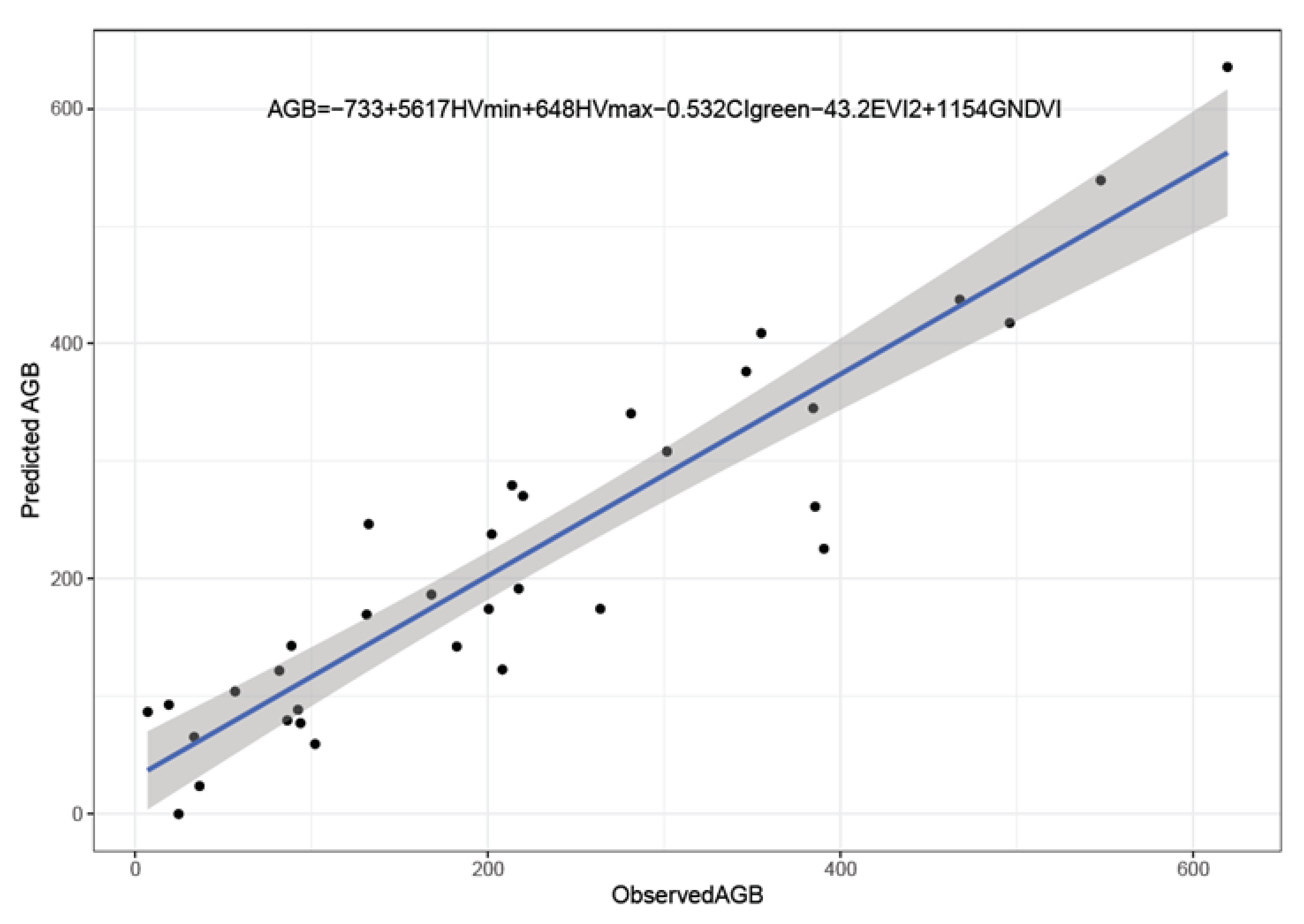
The novel AGB estimates here produced from satellite data show that this information may be generated soon after the event using a simple and well-known regression model (SMLR). However, results must be carefully interpreted being aware of the limited size of test areas and validation samples. The models cover a wide AGB range and are characterized by medium (ALOS2, R2 = 0.65) to high (ALOS2 + S2, R2 = 0.8) accuracy. The modeling differences between SMLR and PLSR algorithms are minimal and do not justify the adoption of an advanced statistical method such as PLSR. L-band SAR data have a limited cost compared to lidar airborne surveys, and satellite data provide a large area coverage with a high revisit time allowing for the production of updated information. Even if the forest biomass increment is slow in time, timber management activities can alter the forest volume and cause errors if old biomass or volume data are used; consequently, using updated data is critical. The use of SAR to estimate AGB is frequently advised to overcome cloud cover issues that affect other data types, as already demonstrated by several authors [
38,
50,
51,
52]. On the other hand, the distortion effects caused by steep slopes in SAR data excluded many forest areas in mountainous regions from the analysis. The use of vegetation indices from Sentinel 2 improved model accuracy but also introduced additional mosaic artifacts and further reduced the area with valid data. In addition, a mosaic based on two years of S2 images had to be generated due to cloud cover issues, requiring additional work steps. Unfortunately, for many areas affected by Vaia damages, it was not possible to produce AGB estimates, and the practical applicability of the method remains only partial over steep mountain ranges.
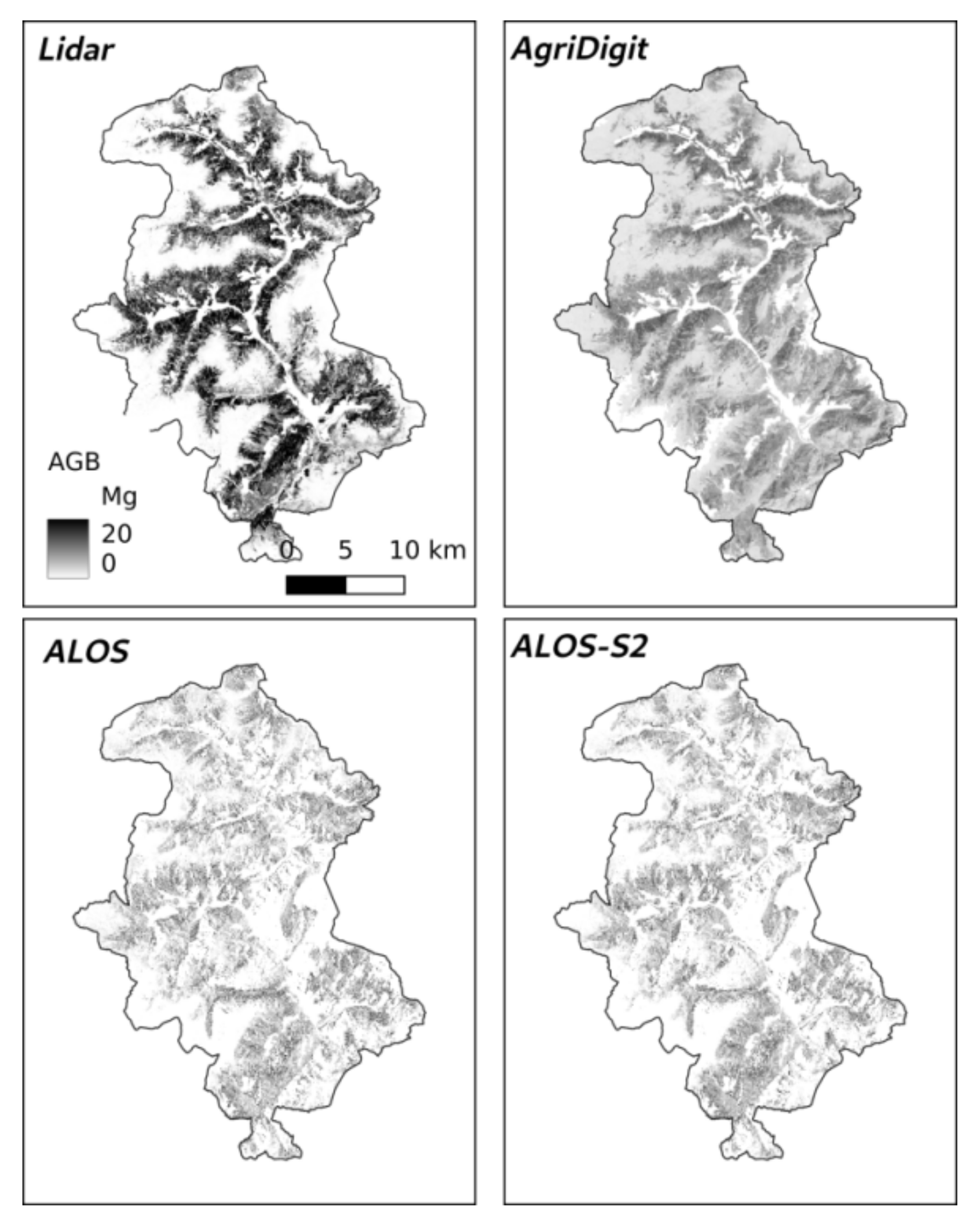
The basic statistics of the four AGB estimates, which are the lidar-based, AgriDigit, and two SAR-based, are different (
Table 2). Considering that the statistics are extracted from different extents where valid data occur, a comparison is challenging. In Trento, where the lidar-based and AgriDigit estimates cover similar areas (92 and 97% of the CLC forest area, respectively), the former shows higher statistics for range, median and quartiles, possibly indicating an underestimation of AGB in the AgriDigit layer. In UMA, only the two SAR-based estimates have similar extent; the one based on ALOS2 data exhibits lower values than the ALOS2 + S2 estimate, except for the average AGB on the third quartile, suggesting that the introduction of Sentinel 2 causes an overestimation of AGB values.
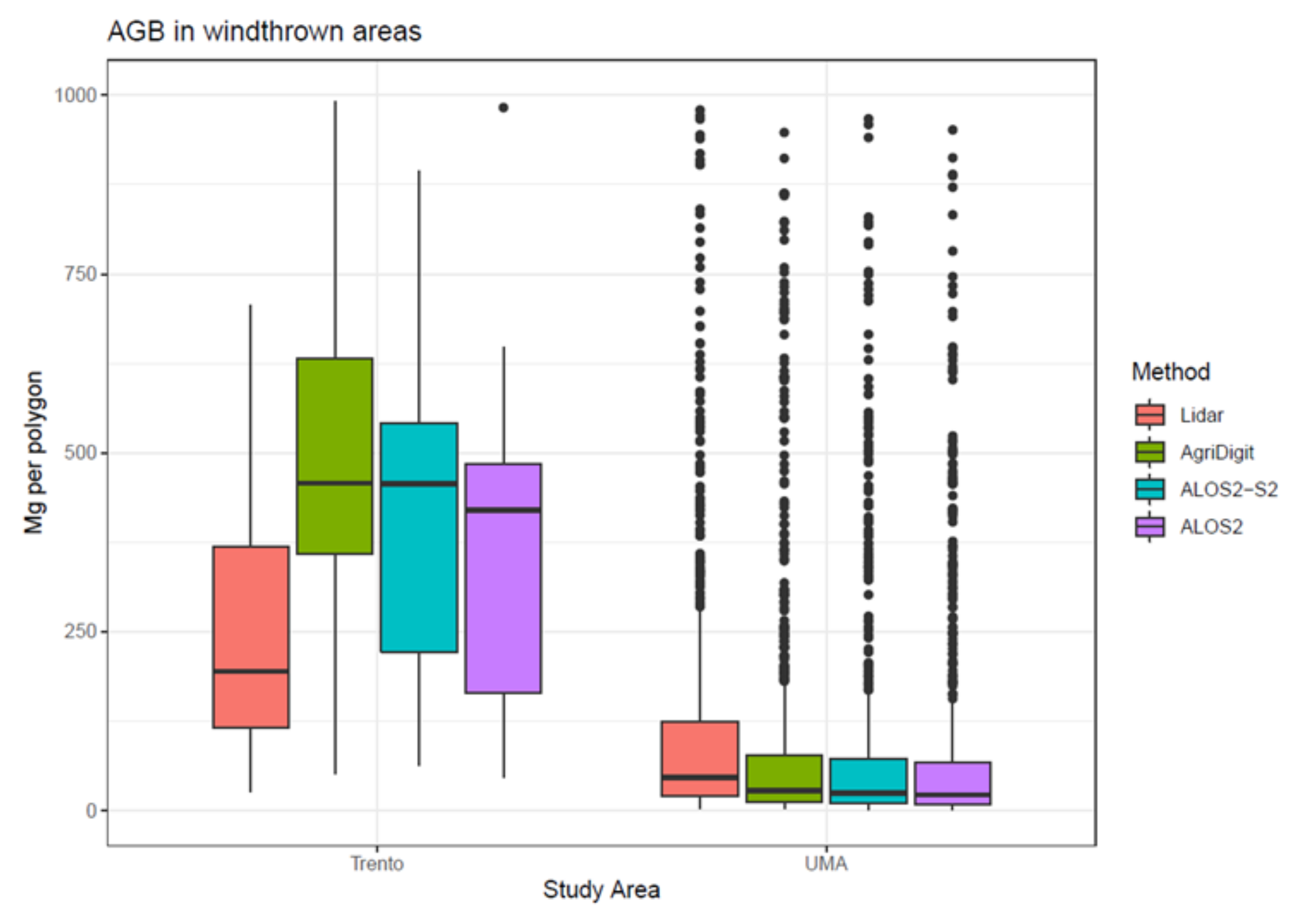
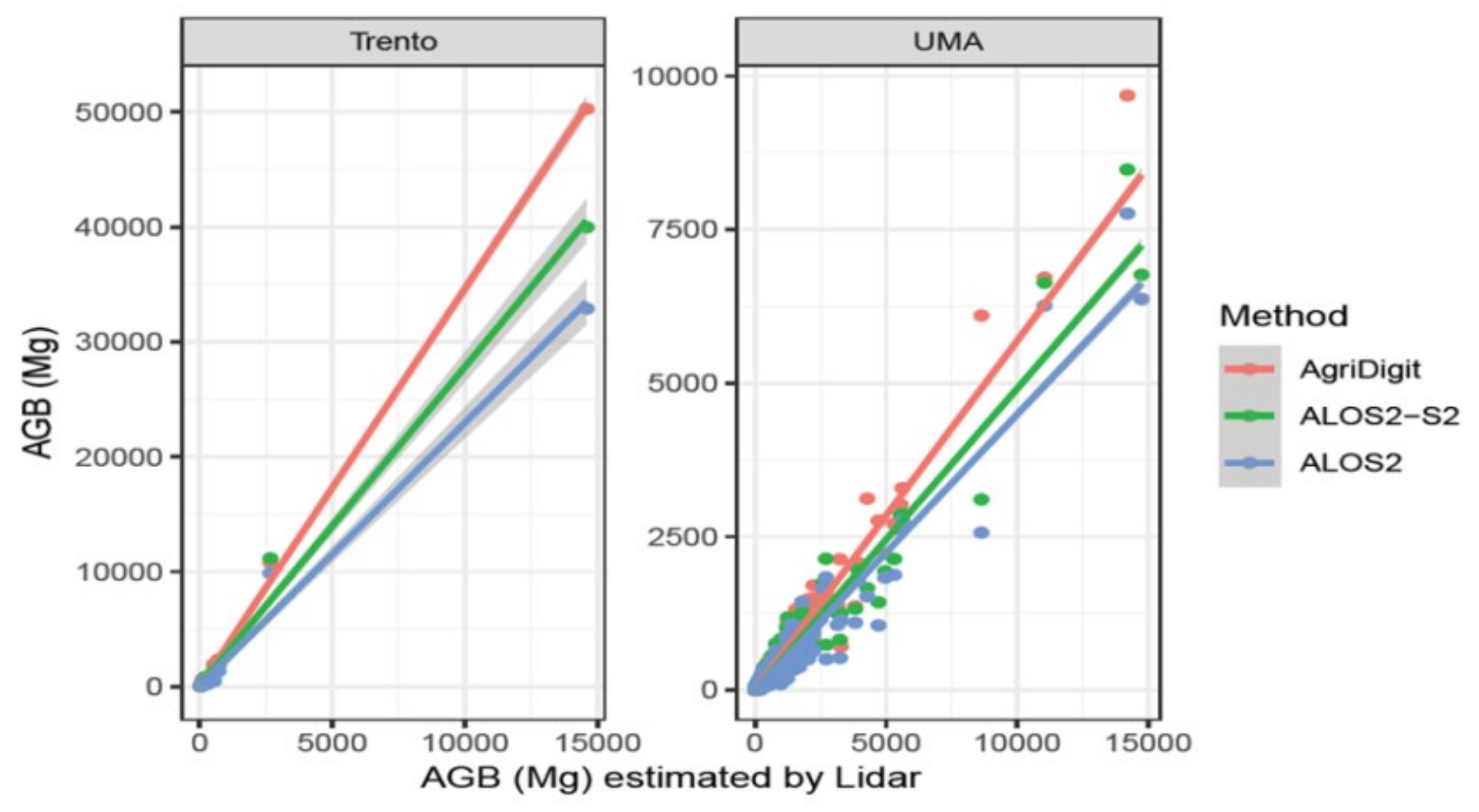
When comparing the amount of AGB occurring in windthrown polygons, that is the information requested to evaluate the forest damages and the amount of timber lost, for Trento obtained significant differences were obtained—according to the pairwise Wilcoxon test—only for the ‘lidar-based—AgriDigit’ pair, with AgriDigit underestimating AGB in comparison to lidar-based estimate, similar to what was derived from the statistics of the overall layers. However, also the ‘lidar-based—ALOS2 + S2’ pair showed a
p-value at the threshold of significance in this area, with ALOS2 + S2 overestimating AGB with respect to lidar. Instead for UMA all the pairs resulted significantly different, except for the ‘ALOS2—ALOS2 + S2’ one. The Uganda country-level study from [
52] suggests that the major source of variation in different AGB estimates is caused by calibration data, and to a lesser degree by remote sensing data used to upscale field values. However, the present research shows different results as the lidar-based and SAR-based estimates use the same calibration datasets but exhibit large differences. In particular, the data in Trento suggest that SAR or SAR + S2 overestimate AGB in windthrown polygons when compared to lidar, while the opposite is observed in UMA.
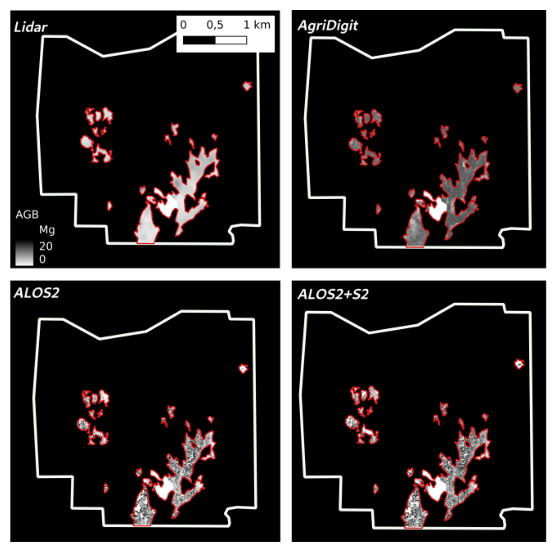
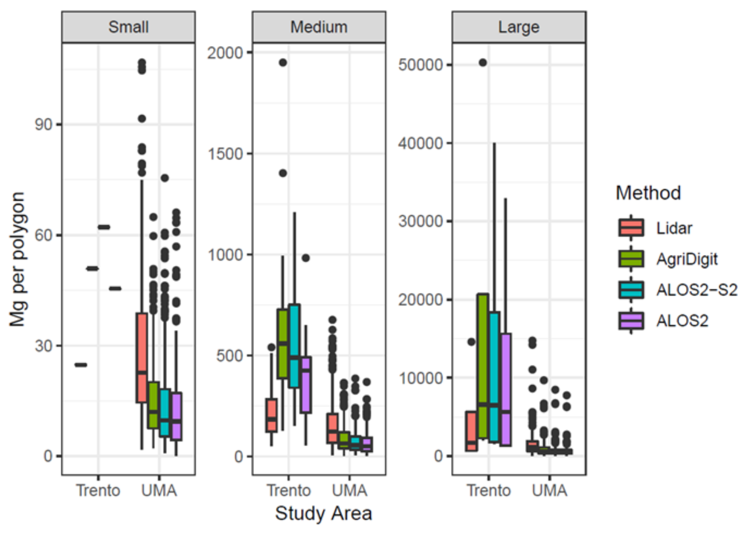
The size effects of the windthrown polygons on AGB estimates was investigate analyzing the AGB values in small, medium, and large polygons, and different results were obtained in Trento and UMA. In Trento, the differences in estimates for medium size polygons were significant only for two pairs (‘lidar-based—AgriDigit’ and ‘lidar-based—ALOS2 + S2’), while no significant differences were found for large polygons. In UMA, instead, most of the estimates differed for both small and medium polygon size; for large polygons, the lidar-based estimates resulted different from all the others, but the ‘AgriDigit—ALOS2 + S2′ pair also significantly differed. These results suggest an effect of the size of the windthrown areas on the estimates, especially in Trento. The reason could be related to edge effects, which are higher in small or medium polygons and can affect both the accuracy of field data collection and the extraction of pixels from the imagery. Edge effects are well known in image classification for reducing accuracy [
53,
54]. Other studies suggested that the different types of remote sensing data, e.g., optical versus SAR, play a role in the production of differing estimates. For instance, [
55] compared AGB maps derived from optical GeoEye-1 and ALOS PALSAR in Nepal, finding that the spatial patterns of AGB were in reasonable agreement at lower elevations, while SAR seems to underestimate AGB values when compared to optical-based estimates in higher elevation zones. Since UMA is characterized by steeper slopes compared to Trento, the observed differences in AGB estimates could be related to both remote sensing data and elevation.
5. Conclusions
One of the major novelty of this research is the comparison of timber loss estimates generated with different data and methods, that provides relevant information to forest managers when called to evaluate the forest damages. The case of Vaia storm is useful to illustrate the situation that forest managers may face in case of an extreme event. Forest managers need to select one method/datasource among the many available to estimate the amount and location of the losses. Here, the available options are examined, assessing limits and advantages, in order to support the decision-making process in real case scenarios.
The notable disagreement among the estimates of timber loss is related to the methods used to produce them, the characteristics of the study areas, and possibly the size of the damaged areas, all of these being sources of uncertainty. Clearly, having large differences among different methods does not help the planning of post-event intervention phases, and highlights the urgent need to define a common national strategy to improve preparedness to forest hazards. The AgriDigit estimate is a notable starting effort, but it must be replicated using recent information, while increasing the calibration dataset over all the forest classes.
Until improved biomass national data will not be available, it is up to forest managers to decide how to quantify the timber loss, according to their knowledge of the local environment. SAR-only or SAR plus optical imagery biomass models are affected by SAR distortion effects in complex morphological terrain, and by the very limited availability of cloud free optical data. In the Vaia case this resulted in a large amount of no data pixels discouraging the adoption of this approach in steep mountain areas. However SAR and optical data could still be valuable data sources in less complex terrains. Lidar -when available- is the best choice to quantify timber loss and was here considered the reference dataset; it suffers from less limitations and has usually high accuracy, but for biomass quantification purpose it is useful only if coupled with proper ground data, allowing to build a biomass estimate. Unfortunately, these conditions are not so frequently met in many European countries.
The availability of a wall-to-wall lidar dataset, together with proper ground data to calibrate the lidar-based model, could solve most limitations. Furthermore, a lidar dataset would be beneficial for many other applications, including hydrogeological and risk-assessment models, or biodiversity assessments. Many EU countries have already implemented this strategy: e.g., Slovenia finalized an open dataset at 5 points per square meter in 2015; Poland, Sweden, and The Netherlands provide nation-wide lidar data through their cartographic offices. New technologies, such as photon counting lidar sensors, may offer a convenient solution to carry out nationwide lidar surveys at defined time intervals.
Considering the frequent impacts on forest resources occurred in the EU in the last years, also related to increased climate change effects, the production of reliable forest stocks data should be the priority for many European countries.


 ,
, 


