Abstract
With the recent proliferation of mobile and wearable devices, wireless power transfer (WPT) has gained attention as an up-and-coming technology to charge these devices. In particular, WPT via magnetic resonance coupling has attracted considerable interest for day-to-day applications since it is harmless to the human body and has relatively long transmission distance. However, it was difficult to be installed into environment (e.g., utensils and furniture) and flexible objects in the living space since the use of flexible coils leads to the decrease in transmission efficiency due to the collapse of the resonance caused by coil deformation. Therefore, this study proposes an automatic resonance compensation system that automatically compensates the inductance variation caused by coil deformation using a circuit that can electronically control the equivalent capacitance (a capacity control circuit), and thereby maintains the resonant state. An experiment was conducted to verify whether the efficiency was maintained when the coil deformed. The results indicated a transmission efficiency nearly as high as that of the ideal resonant state as well as a highly responsive control, and therefore, the proposed system has a good potential for use in real-world applications.
1. Introduction
The proliferation of mobile and wearable devices is making its power management troublesome, and under this circumstance, wireless power transfer (WPT) has gained attention as an up-and-coming technology to charge these devices. In particular, there is a growing interest in the use of WPT by magnetic resonance coupling [1,2,3,4,5,6,7,8] in day-to-day applications because of its broader transmission range compared with electromagnetic induction [9], higher transmission efficiency and relatively low impact on the human body compared with microwaves [10] and laser [11].
However, since rigid coils were mostly used in WPT via magnetic resonance coupling, it was difficult to be installed into environment (e.g., utensils and furniture) and flexible objects in the living space. For this reason, the application of WPT has been limited so far. Here, using flexible and deformable coils instead of rigid coils will open the way to embed power transmission coils into flexible utensils and furniture (and thereby expand the WPT area), as well as flexible objects and devices (and thereby expand the WPT-compatible options). For example, it would be possible to expand the power transfer area by embedding a flexible coil into sofas, reclining chairs, and back cushions. Furthermore, soft objects and devices such as plush toys with monitoring cameras, skin patch/body wrapped biosensors and electrical muscle stimulation (EMS) devices, and haptic gloves could be turned into WPT-compatible by installing a flexible coil. These situations could be indicated graphically as Figure 1a. Looking from the other point of view, attaching flexible coils to home appliances of different shapes and making them WPT-compatible could be another application (Figure 1b). Outside the realm of living spaces, sensors with flexible coils can be attached to the internal wall of pipes to monitor their internal condition [12,13,14,15] (Figure 1c). Therefore, the use of flexible coils will expand the applicability of WPT via magnetic resonance coupling, but so far, this was not widely available due to concerns such as reduction in transmission efficiency.
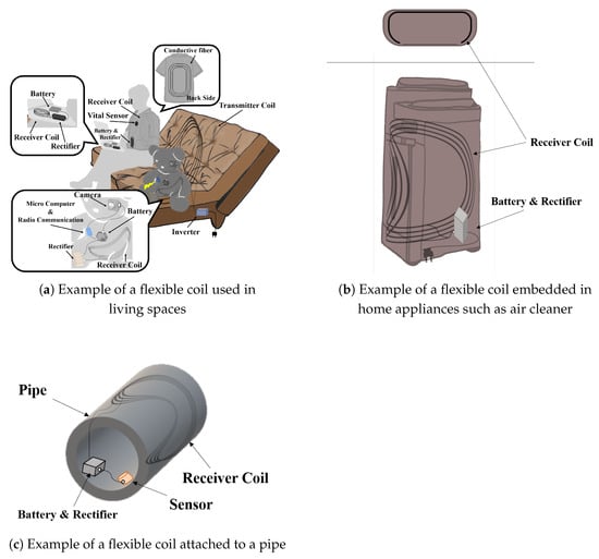
Figure 1.
Examples of applications of WPT using flexible coils. (a) Used in living spaces (b) Embedded in home appliances (c) Attached to a curved shape.
In WPT via magnetic resonance coupling, a condition for a high-efficiency power transfer is that the resonance frequency of the circuit and the frequency of the power source are matching. Thus, it ends up in a decrease in transmission efficiency when the flexible coil is used, since the resonance frequency of the circuit changes due to inductance variation caused by deformation of the flexible coil. Therefore, to supply power wirelessly with high efficiency using flexible coils, it is necessary to set or control the capacitance value of external capacitors to ensure resonance according to the coil shape (inductance value).
To date, there has been not so much research on WPT using flexible coils via magnetic resonance coupling compared to that via electromagnetic induction. Some studies assumed that the shape of the flexible coil does not change. For example, a study that dealt with theoretically calculating self-inductance and mutual inductance of flexible coils of free-form surface to determine the capacitance value of external capacitors was conducted [16]. In contrast, there are studies that considered the shape change of flexible coil as well. For example, one study proposed making design changes such as making the coil smaller or tightening the coil winding to reduce the drop in transmission efficiency due to resonance loss caused by coil shape change [17]. However, there is no guarantee that such design changes can be applied to a power receiver coil, and even if it is possible, a certain efficiency drop will still occur when the shape changes.
Therefore, this study proposes a practical method that automatically controls the capacitance value of external capacitors to counter the efficiency drop caused by the shape change of flexible coils. We propose a method of resonance compensation by automatic control of the capacitance value of external capacitors according to changes in the shape of flexible coils.
The two main contributions of this paper are as follows: First, it offers an automatic resonance compensation system that maintains a high transmission efficiency despite changes in the coil shape in WPT via magnetic resonance coupling using flexible coils. Here, we proposed a simple but practical method which maximize the apparent power ratio using hill-climbing method in order to maximize the transmission efficiency. It should be noted that the capacity control circuit itself was also modified to support serial-serial WPT. Secondly, we demonstrated via actual experiments that the proposed system is able to maintain a level of transmission efficiency nearly as high as that of the ideal resonant state, while it also shows enough control responsiveness.
2. Efficiency Compensation by Capacity Control in Case of Using Flexible Coils
This section looks at how the deformation of a flexible coil used on the power receiver side affects transmission efficiency. Moreover, we verify that the maximum efficiency is achieved during resonance based on the electrical circuit theory. Finally, the effectiveness of efficiency compensation by capacity control is detailed.
Figure 2 shows the equivalent circuit of the series-series (SS) WPT via magnetic resonance coupling dealt with in this paper. Here, as the reactance of the transmitter side does not affect the transmission efficiency (in reality, there is a slight effect due to the presence of internal resistance, but it is ignored) [18], in this study, the reactance of the transmitter side is considered 0 (i.e., transmitter side is in resonant state) for the sake of simplicity and for focusing on the transmission efficiency. Equation (1) shows the formula of transmission efficiency for this case. The changes in the circuit element values due to the coil deformation and the effect of these changes on the transmission efficiency are as follows.
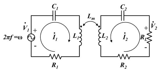
Figure 2.
Equivalent circuit of the series-series (SS) WPT via magnetic resonance coupling.
When the coil on the power receiving side is deformed, the self-inductance of the power receiving side , and the mutual inductance between the power transmitting and receiving sides change. This happens because the coil deformation leads to the change of flux linkage in the coil, while self-inductance is the proportional coefficient between the current flowing in the coil and the flux linkage, and the mutual inductance is the proportional coefficient between the current flowing in one coil and the flux linkage in the other coil in a pair of coils.
As for the mutual inductance , the higher value, which means the stronger magnetic field coupling between the coils, leads to the higher transmission efficiency. On the other hand, as for the self-inductance , the combined reactance with the series-connected capacitor , which is represented as , affects the transmission efficiency as shown in Equation (1). In detail, the maximum value is reached when the receiver side reactance becomes 0.
where
From this, it is natural to come up with a method of resonance compensation that maximizes the transmission efficiency by controlling capacitor against the variation of inductance caused by changes in the flexible coil’s shape and thereby maintains the resonant state (to keep the reactance at 0). This means controlling capacitor as self-inductance changes so that Equation (3) is always satisfied.
In this study, we introduce a simple capacity control circuit that can electronically control the equivalent capacitance value of capacitor and propose an automatic resonance compensation system that maintains the maximum efficiency using this circuit in a fully automatic manner. In the next section, this capacity control circuit and automatic resonance compensation system are detailed.
3. Proposed Automatic Resonance Compensation System
3.1. Overview
The proposed automatic resonance compensation system maintains the resonant state by electronically controlling the equivalent capacitance value of the capacitor against the inductance variation caused by changes in the shape of the flexible coil. This section first details the capacity control circuit that makes the electronic control of equivalent capacitance value possible, and then looks at the resonance compensation algorithm used in case this capacity control circuit is mounted on the receiver side.
3.2. Capacity Control Circuit
3.2.1. Capacity Control Methods
Various methods of electronic control of equivalent capacitance values have been proposed to date, and there are some studies applying these methods to WPT. The first example is an intuitive method that switches the connection of the multiple capacitors arranged in array [19,20]. While easy to implement and control, this method has a limitation that it can only control discrete capacitance values. Then, there is a method that uses voltage controlled capacitors frequently used in the field of communications [21]. While this method realizes continuous capacitance values, the fact that the voltage on the power line itself changes the capacitor value limits its use for low-power transmission.
In contrast to these methods, a method which employ semiconductor switches could realize continuous capacitance values with high power transmission [22,23,24,25,26,27,28,29,30]. The method that uses zero volt switching (ZVS) to reduce switching loss [22] is superior in terms of transmission efficiency, but it must be used alongside an inverter capable of switching control to synchronize the switching timing. However, though the slight unavoidable switching loss occurs, more convenient capacity control method that can be used independently from the inverter switching control is proposed [23,24,25]. To emphasize versatility, we chose to design the capacity control circuit based on this convenient capacity control (hereinafter referred to as “conventional capacity control circuit”).
Conventional capacity control circuit has only been used in parallel-parallel (PP) WPT via magnetic resonance coupling [23,24,25]. Previous studies dedicated to the use of WPT in implantable devices have used it as a component of resonance inverter to draw as much power as possible by adjusting the resonance frequency to that maximizes the transmission efficiency. This frequency varies according to changes in the coupling coefficient due to variations in the distance between transmitter and receiver coils, changes in the load impedance according to the state of charge of the energy storage device, and changes in element constants due to electrical coupling between living tissues [23,24]. In another example, a conventional capacity control circuit was used as a high-power source of medical devices. Here, it was used as a component of resonance inverter to prevent resonance loss due to temperature drift, aging, and manufacturing dispersion [25]. In all these cases, a conventional capacity control circuit was used as a resonance capacitor of a transmitter side parallel resonant circuit in PP WPT via magnetic resonance coupling.
In this study, however, it is used as a resonance capacitor of a receiver side series resonant circuit in SS WPT via magnetic resonance coupling. The reason why SS WPT is chosen instead of topology such as SP WPT is because the optimum load value, which shows the maximum transmission efficiency, appears to be closer to the load values of typical mobile devices.
In this case, it is not possible to apply a conventional capacity control circuit as it is. Therefore, the following section explains the detailed structure of a conventional capacity control circuit also describing the current problem of applying it for SS system, as well as an improvement made into a capacity control circuit so that it can be used in SS system.
3.2.2. Details of the Conventional Capacity Control Circuit and Its Problem in Applying for SS System
Figure 3 shows a conventional capacity control circuit. It is composed of a control capacitor , two semiconductor switches placed at both ends of control capacitor , a fixed base capacitor for voltage reference , and a phase controller (Figure 4).
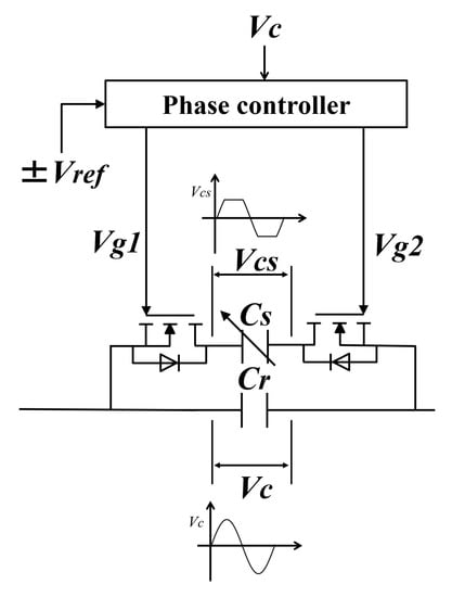
Figure 3.
Configuration of the capacity control circuit.
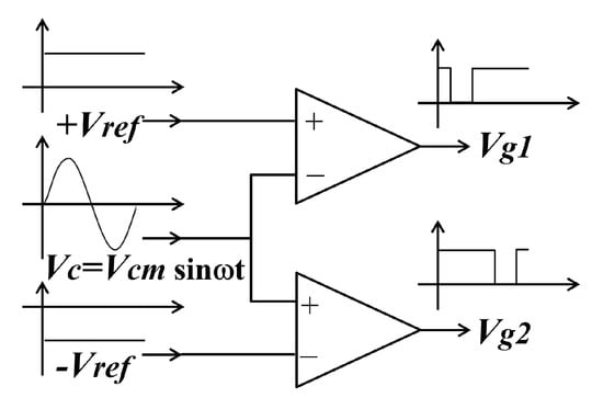
Figure 4.
Detail of the phase controller.
The phase controller compares (terminal voltage of the fixed capacitor ) and control voltage and outputs gate signals and (Figure 5).
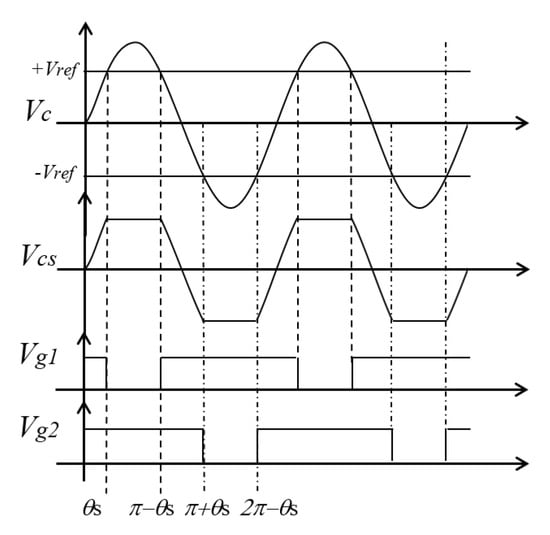
Figure 5.
The waveform , , , and .
This gate signal controls the switches at both ends. With this, the conduction and non-conduction of the control capacitor are switched, and therefore, leads to the changes in (the voltage across the control capacitor ).
By changing , it is possible to control the duty cycle (the ratio of time the capacitor is conductive), and a continuous change of the equivalent capacitance below the original capacity can be realized. The theoretical value of equivalent capacitance could be expressed as Equation (6), using the phase angle parameter shown in Equation (4) that describes the switching timing of the switches linked by the duty cycle. Here, is the amplitude value of .
Equation (6) is derived from Equation (5) which represents that the stored charge integrated over a half cycle is equal for the switching-controlled capacitor and the capacitor that shows the equivalent capacitance value. In other words, assuming that a sinusoidal voltage is applied, the capacitor with an effective capacitance value of stored charge equivalent to that of the control capacitor is called the equivalent capacitance .
The equivalent capacitance value of the entire circuit, , is represented by Equation (7):
In case a conventional capacity control circuit is used as a resonance capacitor of a transmitter-side parallel resonant circuit in PP WPT via magnetic resonance coupling, terminal voltage of the fixed capacitor (which is a reference voltage) is constant, and therefore, the duty cycle and control voltage are in one-to-one correspondence. However, when it is used as a resonance capacitor of the receiver side series resonant circuit in an SS system, the reference voltage varies, and therefore, it is necessary to set control voltage according to reference voltage to realize the desired duty cycle. Hence, it becomes important to improve the conventional capacity control circuit so that it can support changes in the reference voltage.
3.2.3. Improved Capacity Control Circuit
Figure 6 shows a capacity control circuit that can support changes in the reference voltage. The circuit is formed by a capacity controller, a generator of control voltage , and an extractor of terminal voltage . is a control capacitor that changes the equivalent capacitance value and is a base capacitor with fixed value to obtain terminal voltage .
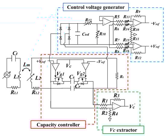
Figure 6.
The entire circuit including the modified capacitance control circuit.
The newly added control voltage generator generates control voltage by rectifing terminal voltage , dividing the voltage by a voltage divider circuit, and passing through the differential amplifier circuit. Here, the gain of differential amplifier circuit is controlled by an electronically controllable resistor (digital potentiometer) ~, and the voltage divider circuit with variable resistors and is inserted to allow the digital potentiometer to be operated in appropriate voltage range.
As the control voltage is generated by multiplying terminal voltage by the differential circuit gain, the duty cycle and differential circuit gain are in one-to-one correspondence regardless of the terminal voltage.
Details on how to determine each resistance value are as follows. First, the relation between and could be described as follows, where we assume that ~ = , ~ holds, and represents the resistance value of digital potentiometer.
Then, determining the control range of the digital potentiometer resistance value as follows,
the control range of the could be expressed as follows.
Incidentally, the terminal voltage extractor works as an adjustment function to define the duty ratio range by balancing the voltage level between the and . Here, the output voltage of the terminal voltage extractor works as the actual reference voltage to determine the duty ratio. If we put the amplitude component of as , the relationship with becomes as follows, where assuming = and = .
Therefore, the duty ratio range could be determined as by setting appropriate resistance values for and to satisfy . Thus, the range of the equivalent capacitance could be derived by Equation (6) and following equation which is the relation between the phase angle parameter and the duty ratio.
3.3. Resonance Compensation Algorithm
This section details the fully automatic resonance compensation method that maintains the maximum efficiency using a capacity control circuit.
Here, the following explanation is based on equivalent circuit expressed as Figure 2. Firstly, the relationship between transmission efficiency and receiver side reactance is expressed by Equation (1); the maximum transmission efficiency is reached when the reactance is 0. Therefore, the basic concept of this technique is to control capacitor with respect to self-inductance (corresponding to the coil shape) so that it satisfies Equation (3). The capacitor is controlled by capacity control circuit introduced above.
Since measuring self-inductance itself is difficult, one of the promising solution is to focus on the fact that the characteristic curve of transmission efficiency relative to capacitor is unimodal and use the hill-climbing method to search for the maximum value. However, in order to derive the transmission efficiency, which is calculated as the ratio of the active power transmitted and received, phase difference measurement between voltage and current which is somewhat complex is required since the active power on the transmitter side is determined by multiplying the power factor calculated from the phase difference by the apparent power. Hence, instead of the active power, we decided to use the apparent power, which can be easily derived as the product of the effective values of voltage and current amplitude. In detail, the ratio of apparent power on the transmitter and receiver sides named as apparent power ratio is introduced and resonance compensation is performed by searching capacitor that maximizes the apparent power ratio . The measurement system becomes simpler in this approach since it appears not necessary to obtain the phase difference.
For this method to function properly, it is necessary that the characteristic curve of the apparent power ratio relative to capacitor is unimodal and becomes resonant state at its peak, and therefore, maximizes transmission efficiency at the same time.
Assuming that the transmitter side is in resonant state, Equation (14) holds according to Kirchhoff’s voltage law:
The currents of transmitter and receiver side and the load voltage of receiver side are expressed as Equations (15)–(17) using input voltage .
Furthermore, the effective value of the input voltage/current and load voltage/current is expressed by Equation (18), and the apparent power of transmitter and receiver side is expressed by Equation (19):
Finally, using Equations (15)–(19), the apparent power ratio is expressed as Equation (20). This equation shows that the characteristic curve of apparent power ratio relative to the reactance of the receiver side is unimodal, and its maximum value is reached when the reactance is 0. This agrees with the condition for the maximum transmission efficiency to be reached. Therefore, it was proved that maximizing the apparent power ratio with the capacity control using the hill-climbing method is valid.
where
Figure 7 shows the configuration of the automatic resonance compensation system. The effective values of voltage and current were obtained by measurement devices in both transmitter and receiver side, and then the computer calculates apparent power ratio , and finally adjusts the values of the variable resistors determining the equivalent capacitance using the hill-climbing method.
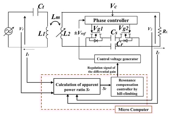
Figure 7.
Configuration of the automatic resonance compensation system.
A detailed flow of the hill-climbing method is shown in Figure 8. Apparent power ratio at the previous time and the current time are compared, and if the efficiency increased, the direction of adjustment of the capacitance value (the varying direction of the variable resistor value) was maintained, and if the efficiency decreased, it was inverted. In addition, when the efficiency oscillated, it was converged to the maximum value by decreasing the amount of capacitance value adjustment.
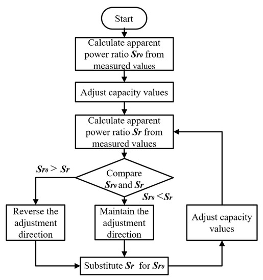
Figure 8.
Flowchart of the hill-climbing method.
4. Experiment
4.1. Experimental System
Figure 9 and Figure 10 show the experimental configuration of the automatic resonance compensation system and the experimental environment itself. The power input from the function generator flows through the power transmitter coil, the power receiver coil, the capacity control circuit, and finally being supplied to the load resistance. The voltage and current of the transmitter and receiver side were measured by an oscilloscope (TBS2104) through a differential voltage probe and a current probe.
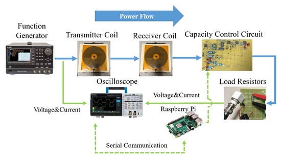
Figure 9.
Experimental configuration.
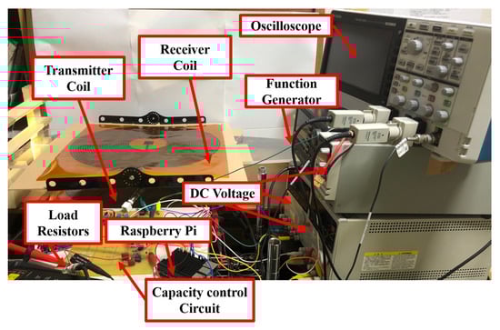
Figure 10.
Experimental environment.
The circuit parameters in Figure 6 are shown in Table 1. The flexible deformable coil with a radius of 20 cm and 25 turns were used. A resonance capacitor connected in series to the flexible coil on the power transmitter side is adjusted to realize resonant state at 85 kHz. The capacity control circuit was connected in series to the flexible coil in the receiver side.

Table 1.
Circuit Parameters.
The details of the capacity control circuit are as follows. In the control voltage generator, the operational amplifier gain was adjusted by the digital potentiometer used in ~. Moreover, a voltage-dividing resistor was used so that the rated voltage of the digital potentiometer was not exceeded, and to ensure that the division was done correctly, it was insulated by inserting a voltage follower between the partial resistance and the digital potentiometer. To prevent the semiconductor switches from malfunctioning due to a possible voltage shortage in the gate signals of the phase controller, we built a gate driver circuit with a photocoupler (TLP2361). An N-Channel MOSFET (2n7002k) was used as the semiconductor switch of the capacity control circuit.
Raspberry Pi 4 was used as a micro computer. The measured voltage/current of the transmitter and receiver side were input to the computer and the apparent power ratio is calculated. The hill-climbing method is running in the computer and the control value of the digital potentiometer was determined using the apparent power ratio as input. Then, the equivalent capacitance value of the control capacitor was regulated by controlling the digital potentiometer through SPI communication.
Here, it should be noted that the voltage and current of the transmitter should be wirelessly communicated to the receiver in the actual applications. The time delay could be calculated as 1.4 ms per control cycle, assuming transmitted data of 10 bytes (80 bits) and the typical transmission rate of 57,600 bps in Xbee which is common device for wireless communication. Since this delay is small enough compared to the original control cycle of 53 ms, we decided to ignore implementing the wireless communication device in the current system, which focuses in verifying the operation of the proposed efficiency compensation method.
4.2. Efficiency Compensation Relative to the Shape Change of a Flexible Coil
A comparative experiment was carried out to verify the performance of automatic resonance compensation when the shape of a coil changed under three conditions: “Ideal resonance (manually set ideal capacitance value)”, “automatic resonance compensation (the proposed method)”, and “non-resonant (fixed capacitance value)”. The transmission distance between the coils was a horizontal gap of 105 mm.
In terms of the electric circuit model, the purpose of the experiment is to verify the effectiveness of proposed method which automatically controls to compensate the efficiency by maintaining the resonance when receiver inductance changes. Therefore, any flexible coil bending pattern which can dynamically change inductance was acceptable. Thus, as illustrated in Figure 11, the transmission efficiency was measured when the flexible coil on the receiver side was bent from 0 to 120 degrees with an increment of 10 degrees.
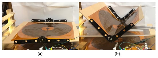
Figure 11.
(a) Bending angle: 0 degrees; (b) Bending angle: 90 degrees.
First, as the ideal resonance condition, for each bending angle of the flexible coil, the capacitance values of resonance capacitors connected in series were adjusted so that the entire receiver side resonated at 85 kHz. The adjustment was made manually using an impedance analyzer.
Next, as the non-resonant condition, the capacitance value of the resonance capacitors was fixed to a value with which the flexible coil resonated at 85 kHz in a flat condition (with a bending angle of 0 degrees). With this, when the shape of the flexible coil is changed, it appears to be a non-resonant state.
Lastly, as the automatic resonance compensation condition, the automatic resonance compensation using the hill-climbing method mentioned above was applied, and the results were measured at a steady state, after a considerable amount of time.
Figure 12 shows how the transmission efficiency changed with respect to the coil bending angle. In the ideal resonance case, the capacitor was adjusted to the coil’s bending angle so that it was always at the resonant state, and the transmission efficiency was maximum. In contrast, in the non-resonant case, as the flexible coil’s bending angle increased, transmission efficiency decreased significantly. In the automatic resonance compensation case, the efficiency drop relative to the increasing bending angle was suppressed, and the efficiency varied almost like the case of ideal resonance. When the bending angle was 120 degrees, the transmission efficiency improved by 11.4% compared with the non-resonant case.
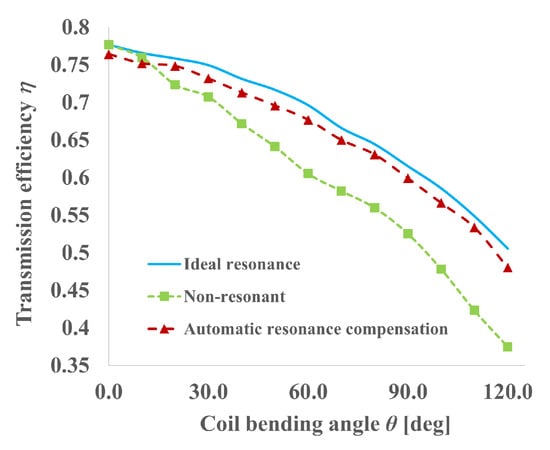
Figure 12.
Changes in the transmission efficiency against the coil bending angle under each circuit condition.
However, it should be noted that some part of additional power consumption due to the introduction of the capacitance control circuit were neglected. Therefore, the following is supplementary information on power consumption.
The additional power consumption in detail is considered to be four points: the driving power of the microcontroller, the switching loss, the detection loss in the phase controller, and the driving power of the operational amplifier. Here, the microcomputer (or control unit which works as so) is usually used in the conventional magnetic field resonance WPT system, and therefore, it could be ignored as an increase in power consumption. In addition, the loss of wave detection in the phase controller could be suppressed to negligible level by using a sufficiently large resistance. Therefore, the main part of the additional power consumption is considered to be the switching loss and the driving power of the operational amplifier. Here, the switching loss appears to be proportional to the transmission power, while driving power of the operational amplifier is considered to be below a certain value. Thus, the experimental results (Figure 12) are derived by accounting only the switching loss as the loss. This means that if the difference of received power in non-resonant case and automatic resonance compensation case is larger than the driving power of the operational amplifier, it is worth implementing the proposed circuit. In the practical case, this could be easily satisfied when the transmitted power is large enough.
Just for reference, the power delivered to the load with respect to the bending angle of the coil for automatic resonance compensation case is shown in Figure 13. It should be noted that since this paper focused on the proposal and basic evaluation of an automatic resonance compensation for WPT using flexible coils, the practicality of the power level was not considered. Therefore, as a future task, we will seek to increase the transmission power for applying the system to real world applications.
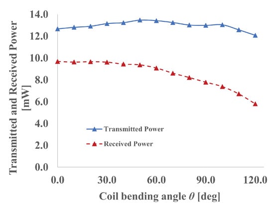
Figure 13.
Changes in power delivered to the load against the coil bending angle under automatic resonance compensation condition.
4.3. Responsiveness of the Automatic Resonance Compensation
The next experiment was designed to verify the responsiveness of automatic resonance compensation. First, the capacity control circuit was turned on and put in the resonant state without deforming the flexible coil. Then, the flexible coil was bent 90 degrees while turning off the capacity control circuit (equivalent capacitance value was kept constant in this condition). Due to this, the coil’s self-inductance varies, and the resonant state was intentionally lost. Finally, the capacity control circuit was turned on again to observe the transition to the resonant state. We verified the time variation, from the moment the circuit was turned on again until the resonant state was reached, of transmission efficiency , apparent power ratio , phase difference of voltage and current , and total capacitance value .
The experiment results are shown in Figure 14 and Figure 15. As time passes, transmission efficiency improved and the phase difference approached 0, and in response, apparent power ratio and transmission efficiency gradually approximated. The total equivalent capacitance converged in about 1 s and the phase difference at the moment of convergence was about 3 degrees, which is 0.9986 if converted to a power factor. Therefore, it could be said that the resonant state has been restored.
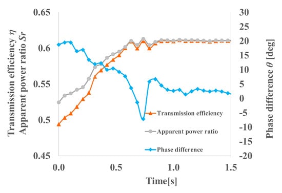
Figure 14.
Time variation of apparent power ratio , transmission efficiency and phase difference.
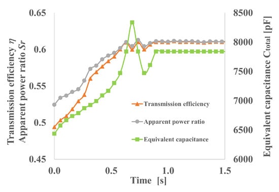
Figure 15.
Time variation of apparent power ratio , transmission efficiency and equivalent capacitance value .
5. Conclusions
In this study, we proposed an automatic resonance compensation system for WPT via magnetic resonance coupling using flexible coils, which maintains high transmission efficiency against coil shape changes.
The system works to compensate the collapse of the resonance caused by coil deformation by controlling the equivalent capacitance to maximize the apparent power ratio. To support serial-serial WPT, a feedback circuit was added to the conventional capacity control circuit to control the duty cycle regardless of the reference voltage.
In addition, through actual experiments, we demonstrated that the transmission efficiency was greatly improved compared to the non-resonant state and was maintained at a level comparable to that of ideal resonance, and also that the system showed certain degree of response.
Here, the change in transmission efficiency was measured when the flexible coil was bent in 10-degree increments ranging from 0 to 120 degrees, and succeeded in improving the efficiency by 11.4% compared to the non-resonant state at a bending angle of 120 degrees.
We also confirmed that the time response in restoring the resonant state after the coil was bent at 90 degrees was about 1 s. This means that the current hill-climbing method works fine if the coil shape fluctuates with a cycle of motion sufficiently slower than 1 s, but fails to track it if the fluctuation is much faster than 1 s. Thus, improving the control response might be an future issue in some applications requiring quite high response.
The future works are as follows. First of all, in actual applications, the output voltage from the inverter is not always a sine wave, but often a signal such as square wave. Since the impedance of the circuit depends on the frequency of the signal, the phase difference of the voltage and current is not constant for the fundamental wave and harmonics of different orders, which are the components of the square wave, and therefore, the apparent power cannot be defined. Therefore, the proposed method of maximizing the apparent power ratio by capacity control using the mountain-climbing method fails in this case. In such a case, maximizing the transmission efficiency directly by the mountain-climbing method might be a good alternative. This should be verified through actual experiments in the future. Moreover, wireless communication should be introduced to send the voltage and current of the transmitter side to the receiver side in the future system. Finally, as an important future task, we will seek to increase the transmission power for applying the system to real world applications.
Author Contributions
Conceptualization, S.N.; methodology, S.N., K.B. and T.M.; data curation, S.N. and K.B.; investigation, S.N. and K.B.; formal analysis, S.N. and K.B.; visualization, K.B.; writing—original draft, S.N., K.B. and T.M.; writing—review and editing, S.N.; supervision, S.N.; project administration, S.N.; funding acquisition, S.N. All authors have read and agreed to the published version of the manuscript.
Funding
This study was supported by the SCOPE (Strategic Information and Communications R & D Promotion Program) No. 205006003 of Ministry of Internal Affairs and Communications and the JSPS KAKENHI 18K04085.
Institutional Review Board Statement
Not applicable.
Informed Consent Statement
Not applicable.
Data Availability Statement
Not applicable.
Conflicts of Interest
The authors declare no conflict of interest.
References
- Chen, L.; Liu, S.; Zhou, Y.C.; Cui, T.J. An optimizable circuit structure for high-efficiency wireless power transfer. IEEE Trans. Ind. Electron. 2013, 60, 339–349. [Google Scholar] [CrossRef]
- Sample, A.P.; Meyer, D.A.; Smith, J.R. Analysis, experimental results, and range adaptation of magnetically coupled resonators for wireless power transfer. IEEE Trans. Ind. Electron. 2011, 58, 544–554. [Google Scholar] [CrossRef]
- Duong, T.P.; Lee, J.W. Experimental Results of High-Efficiency Resonant Coupling Wireless Power Transfer Using a Variable Coupling Method. IEEE Microw. Wirel. Compon. Lett. 2011, 21, 442–444. [Google Scholar] [CrossRef]
- Kim, J.; Choi, W.S.; Jeong, J. Loop Switching Technique for Wireless Power Transfer Using Magnetic Resonance Coupling. Prog. Electromagn. Res. 2013, 138, 197–209. [Google Scholar] [CrossRef]
- Imura, T.; Hori, Y. Maximizing air gap and efficiency of magnetic resonant coupling for wireless power transfer using equivalent circuit and Neumann formula. IEEE Trans. Ind. Electron. 2011, 58, 4746–4752. [Google Scholar] [CrossRef]
- Kurs, A.; Karalis, A.; Moffatt, R.; Joannopoulos, J.D.; Fisher, P.; Soljac, M. Wireless Power Transfer via Strongly Coupled Magnetic Resonances. Science 2007, 317, 83–86. [Google Scholar] [CrossRef]
- Nakamura, S.; Koma, R.; Hashimoto, H. Efficient Wireless Power Transmission based on Position Sensing using Magnetic Resonance Coupling. SICE J. Control Meas. Syst. Integr. 2012, 5, 153–161. [Google Scholar] [CrossRef]
- Nakamura, S.; Namiki, M.; Sugimoto, Y.; Hashimoto, H. Q Controllable Antenna as a Potential Means for Wide-Area Sensing and Communication in Wireless Charging via Coupled Magnetic Resonances. IEEE Trans. Power Electron. 2017, 32, 218–232. [Google Scholar] [CrossRef]
- Jang, Y.; Jovanovic, M.M. A contactless electrical energy transmission system for portable-telephone battery chargers. IEEE Trans. Ind. Electron. 2003, 50, 520–527. [Google Scholar] [CrossRef]
- Farinholt, K.M.; Park, G.; Farrar, C.R. RF Energy Transmission for a Low-Power Wireless Impedance Sensor Node. IEEE Sens. J. 2009, 9, 793–800. [Google Scholar] [CrossRef]
- Kawashima, N.; Takeda, K. Laser energy transmission for a wireless energy supply to robots. Robot. Autom. Constr. 2008, 10, 373–380. [Google Scholar]
- Yang, D.X.; Hu, Z.; Zhao, H.; Hu, H.F.; Sun, Y.Z.; Hou, B.J. Through-Metal-Wall Power Delivery and Data Transmission for Enclosed Sensors: A Review. Sensors 2015, 15, 31581–31605. [Google Scholar] [CrossRef] [PubMed]
- Yamakawa, M.; Mizuno, Y.; Ishida, J.; Komurasaki, K.; Koizumi, H. Wireless power transmission into a space enclosed by metal walls using magnetic resonance coupling. Wirel. Eng. Technol. 2014, 5, 19–24. [Google Scholar] [CrossRef]
- Shimamura, K.; Komurasaki, K. Wireless power transmission into metallic tube using axial slit for infrastructure diagnostics. Wirel. Eng. Technol. 2015, 6, 50–60. [Google Scholar] [CrossRef]
- Shimamura, K.; Koizumi, M.; Mizuno, Y.; Komurasaki, K. Effect of Axial Slit on Metallic Tube for Wireless Power Transfer via Magnetic Resonance Coupling: Application of Magnetic-Resonance Coupling Techniques for Infrastructure Diagnostics. Electr. Eng. Jpn. 2016, 197, 46–54. [Google Scholar] [CrossRef]
- Hou, T.; Xu, J.; Elkhuizen, W.S.; Wang, C.C.L.; Jiang, J.; Geraedts, J.M.P.; Song, Y. Design of 3D Wireless Power Transfer System Based on 3D Printed Electronics. IEEE Access 2019, 7, 94793–94805. [Google Scholar] [CrossRef]
- Wen, F.; Jing, F.; Li, Q.; Li, R.; Liu, L.; Chu, X. Curvature Angle Splitting Suppression and Optimization on Nonplanar Coils Used in Wireless Charging System. IEEE Trans. Power Electron. 2020, 35, 9070–9081. [Google Scholar] [CrossRef]
- Imura, T.; Hori, Y. Unified Theory of Electromagnetic Induction and Magnetic Resonant Coupling. IEEJ Trans. Ind. Appl. 2015, 135, 697–710. [Google Scholar] [CrossRef]
- Beh, T.C.; Kato, M.; Imura, T.; Oh, S.; Hori, Y. Automated impedance matching system for robust wireless power transfer via magnetic resonance coupling. IEEE Trans. Ind. Electron. 2013, 60, 3689–3698. [Google Scholar] [CrossRef]
- Lim, Y.; Tang, H.; Lim, S.; Park, J. An adaptive impedance-matching network based on a novel capacitor matrix for wireless power transfer. IEEE Trans. Power Electron. 2014, 60, 4403–4413. [Google Scholar] [CrossRef]
- Porto, R.W.; Brusamarello, V.J.; Pereira, L.A.; Sousa, F.R. Fine tuning of an inductive link through a voltage-controlled capacitance. IEEE Trans. Power Electron. 2017, 32, 4115–4124. [Google Scholar] [CrossRef]
- Zhang, J.; Zhao, J.; Zhang, Y.; Deng, F. A Wireless Power Transfer System with Dual Switch-Controlled Capacitors for Efficiency Optimization. IEEE Trans. Power Electron. 2020, 35, 6091–6101. [Google Scholar] [CrossRef]
- Si, P.; Hu, A.P.; Malpas, S.; Budgett, D. A frequency control method for regulating wireless power to implantable devices. IEEE Trans. Biomed. Circuits Syst. 2008, 2, 22–29. [Google Scholar] [CrossRef] [PubMed]
- Mohamadi, T. Working frequency in wireless power transfer for implantable biomedical sensors. In Proceedings of the 2011 International Conference on Electrical Engineering and Informatics, Bandung, Indonesia, 17–19 July 2011; pp. 1–5. [Google Scholar]
- Denieport, R.; Rodes, F.; Zhang, M.; Wang, X.; Ren, X. Medical power generator using a voltage mode resonant converter controlled by a synchronous switched capacitor is MRI compatible. In Proceedings of the 21st IEEE International Conference on Electronics, Circuits and Systems (ICECS), Marseille, France, 7–10 December 2014; pp. 530–533. [Google Scholar]
- Rodes, F.; Zhang, M.; Denieport, R.; Wang, X. Optimization of the Power Transfer Through Human Body With an Auto-Tuning System Using a Synchronous Switched Capacitor. IEEE Trans. Circuits Sysems II 2015, 62, 129–133. [Google Scholar] [CrossRef]
- Driscol, S.D.O. A mm-sized implantable power receiver with adaptive matching. In Proceedings of the IEEE Sensors, Waikoloa, HI, USA, 1–4 November 2010; pp. 83–88. [Google Scholar]
- Dissanayake, T.; Budgett, D.; Hu, A.P.; Malpas, S.; Bennet, L. Transcutaneous Energy Transfer System for Powering Implantable Biomedical Devices. In Proceedings of the 13th International Conference on Biomedical Engineering, Singapore, 3–6 December 2008; pp. 235–239. [Google Scholar]
- Si, P.; Hu, A.; Budgett, D.; Malpas, S.; Yang, J.; Gao, J. Stabilizing the operating frequency of a resonant converter for wireless power transfer to implantable biomedical sensors. In Proceedings of the 1st International Conference on Sensing Technology, Palmerston North, New Zealand, 21–23 November 2005; pp. 477–482. [Google Scholar]
- Su, Y.G.; Zhang, H.Y.; Wang, Z.H.; Hu, A.P.; Chen, L.; Sun, Y. Steady-State Load Identification Method of Inductive Power Transfer System Based on Switching Capacitors. IEEE Trans. Power Electron. 2015, 30, 6349–6355. [Google Scholar] [CrossRef]


Publisher’s Note: MDPI stays neutral with regard to jurisdictional claims in published maps and institutional affiliations. |
© 2021 by the authors. Licensee MDPI, Basel, Switzerland. This article is an open access article distributed under the terms and conditions of the Creative Commons Attribution (CC BY) license (https://creativecommons.org/licenses/by/4.0/).