Transient Analysis of Multiphase Transmission Lines Located above Frequency-Dependent Soils

Abstract

This paper evaluates the influence of frequency-dependent soil conductivity and permittivity in the transient responses of single- and double-circuit transmission lines including the ground wires subjected to lightning strikes. We use Nakagawa’s approach to compute the ground-return impedance and admittance matrices where the frequency-dependent soil is modeled using Alípio and Visacro’s model. We compare some elements of these matrices with those calculated by Carson’s approach which assumes the frequency constant. Results show that a significant difference can be obtained in high resistive soils for these elements in impedance and admittance matrices. Then, we compute the transient responses for single- and double-circuit lines with ground wires located above soils of 500, 1000, 5000, and 10,000 Ω·m considering the frequency constant and frequency-dependent parameters generated for two lightning strikes (subsequent stroke and Gaussian pulse). We demonstrate that the inclusion of frequency dependence of soil results in an expressive reduction of approximately 26.15% and 42.75% in the generated voltage peaks in single- and double-circuit lines located above a high-resistive soil. These results show the impact of the frequency-dependent soils that must be considered for a precise transient analysis in power systems.

1. Introduction

In recent years, several authors have studied the impact of the frequency dependence of electrical ground conductivity (${\sigma }_{\mathrm{g}}$) and ground relative permittivity (${\epsilon }_{\mathrm{rg}}$) in the calculation of electromagnetic transients, especially those developed by lightning strikes on overhead multiphase transmission lines (TLs) or on grounding systems [1,2,3,4,5].

In 1930, Ratcliffe et al. introduced one of the first laboratory measurements of effective conductivity ${\sigma }_{\mathrm{g}}$ and relative permittivity ${\epsilon }_{\mathrm{rg}}$ of the soil in radio frequencies [6]. In 1933, Smith-Rose presented a set of systematic measurements considering diverse soil samples [7]. Decades later, between 1964 and 1967, Scott proposed the first set of mathematical expressions to calculate the electrical parameters of the soil (${\sigma }_{\mathrm{g}}$ and ${\epsilon }_{\mathrm{rg}}$) [8]. In the 70s, based on Scott’s formulae, Longmire and Smith proposed a semi-theoretical model, the Universal Soil Model [9]. At the same time, Messier presented an empirical model to calculate ${\sigma }_{\mathrm{g}}$ and ${\epsilon }_{\mathrm{rg}}$ [10]. During the 1980s and 1990s, Visacro [11] and Portela [12] proposed a set of equations to calculate soil parameters between 100 Hz and 2 MHz based on laboratory measurements of diverse soil samples. More recently, Visacro and Alípio introduced two models based on field measurements. The first one uses fitting techniques to obtain formulae for the calculation of soil parameters [13,14]. The second model combines field measurements with electromagnetic theory and causality requirements into a physical model [15].

Researches had evaluated the effects of the frequency dependence of ${\sigma }_{\mathrm{g}}$ and ${\epsilon }_{\mathrm{rg}}$ in grounding systems subject to lightning current [5], transient responses on distribution networks near lightning strikes [1], and overvoltages subject to lightning strikes [2], respectively. Based on previous research, the International Council on Large Electric Systems (CIGRE) published Brochure 781 [16] containing the main physical aspects related to the frequency dependence of ${\sigma }_{\mathrm{g}}$ and ${\epsilon }_{\mathrm{rg}}$, its influence on the transient response of electrical systems due to lightning strikes, and recommendations to consider the above in practical engineering applications [16].

Considering ground-return effect is crucial when evaluating the propagation of voltage and current waves in overhead TLs [17]. In this regard, it is also important to include the frequency dependence of ${\sigma }_{\mathrm{g}}$ and ${\epsilon }_{\mathrm{rg}}$. However, most electromagnetic transient (EMT)-type simulators compute the ground impedance using Carson’s formula, which assumes that the ground conduction current is much larger than the displacement current and excludes the frequency dependence of soil electrical parameters [18]. These assumptions can generate errors in the simulation of soils with high resistivity and applications involving high-frequency phenomena, such as transients caused by lightning strikes on transmission lines. Some papers consider the frequency dependence of ${\sigma }_{\mathrm{g}}$ and ${\epsilon }_{\mathrm{rg}}$ during line energization [18,19,20]. However, authors only consider one type of soil, which makes it difficult to generalize results.

Concerning the transient analysis of transmission lines located on frequency-dependent soils, we highlighted some works. In [21], De Conti et al. analyze the transient voltages in a 3.6 km single and bi-phase transmission lines without ground wire located on soil of 10,000 Ω·m. In [22], De Conti et al. present the transient voltages for two different single and bi-phase transmission lines without ground wires of 0.6 km and 1.8 km in length located on soils of 100, 1000 and 10,000 Ω·m. In [23], Moura et al. analyze the influence of the frequency dependence of ground electrical parameters in terms of the p.u.l. longitudinal impedance and transversal admittance for a single-circuit three-phase transmission line with ground wire. In [24], considering a set of measurements, He et al. investigate the impact of the frequency effect of ${\sigma }_{\mathrm{g}}$ and ${\epsilon }_{\mathrm{rg}}$ on the calculation of line parameters. However, their analysis does not extend to the time domain. In [25], Papadopoulos et al. investigate the impact of frequency-dependent soil parameters on the propagation of transients in a 10 km overhead three-phase transmission line without ground wires. However, authors only analyze simple configurations corresponding to one or two ground wires because their focus is on the analysis of transients in overhead distribution networks. In [4], Salarieh and Kordi show that the backflashover rate estimation of a transmission tower with the grounding electrodes buried in lossy ground is affected by the frequency-dependent soil electrical parameters.

Considering the above works, it is noted that proper grounding modeling has been widely studied in the literature. However in these studies, the transient analyses are performed only for short transmission lines, typically related to distribution power systems. Thus, we understand that a more extensive analysis on the transient responses for commonly multiphase transmission lines (including the ground wires) located on the frequency-dependent soil electrical parameters are need. This objective of this paper is to evaluate the impact of frequency-dependent soil parameters in the transient responses of multiphase transmission lines generated by lightning strikes. First, we calculate the longitudinal impedance and transversal admittance matrices where the ground-return elements are computed by Nakagawa’s approach. The advantage of this approach consists of that the frequency dependence of soil parameters can be included for the analysis. We use the soil modeling proposed by Alípio and Visacro’s. We compare this results with those computed by Carson’s approach which assumes the frequency-constant soil parameters obtained for soils of moderate and high resistive soils. It is demonstrated that for high-resistive soils, a significant difference can be noted in the elements of the impedance and admittance matrices. We show the effects of both approaches in time-domain simulations of high-frequency transients (subsequent return stroke and 1 MHz Gaussian pulse) for diverse soil resistivity in single and double-circuits three-phase transmission lines of 5 km and 50 km in length considering two ground wires at the top of each the tower. Results demonstrated that an expressive difference at the transient peaks can be obtained when the soil is models by its frequency-dependent parameters. As shown, a reduction of 26.15% and of 42.75% in the voltage peaks in a single- and double-circuit lines located above a high-resistive soil are computed for the Gaussian pulse. As contribution of this paper, we analyse the transient responses generated by fast-front disturbances on single and double-circuit transmission lines with ground wires located above high resistive soils in a more realistic line configuration and length.We also show that the proper modeling of soil affects significantly the transient analysis.

This paper is organized as follows: Section 2 presents the equations used to compute multiconductor line parameters. Section 3 shows the Alípio and Visacro’s equations used in this paper to calculate the frequency-dependent soil electrical parameters. Section 4 describes the subsequent return stroke and Gaussian pulse waveforms that we use to represent lightning strikes. In Section 5, we present our methodology in steps to compute the frequency-domain responses. In Section 6, we combine different TL topologies and ground parameters and calculate the line parameters of each combination. Then we simulate these TLs subject to the impulsive currents presented in Section 4 and discuss the results obtained. Finally, Section 7 presents the major conclusions of this paper.

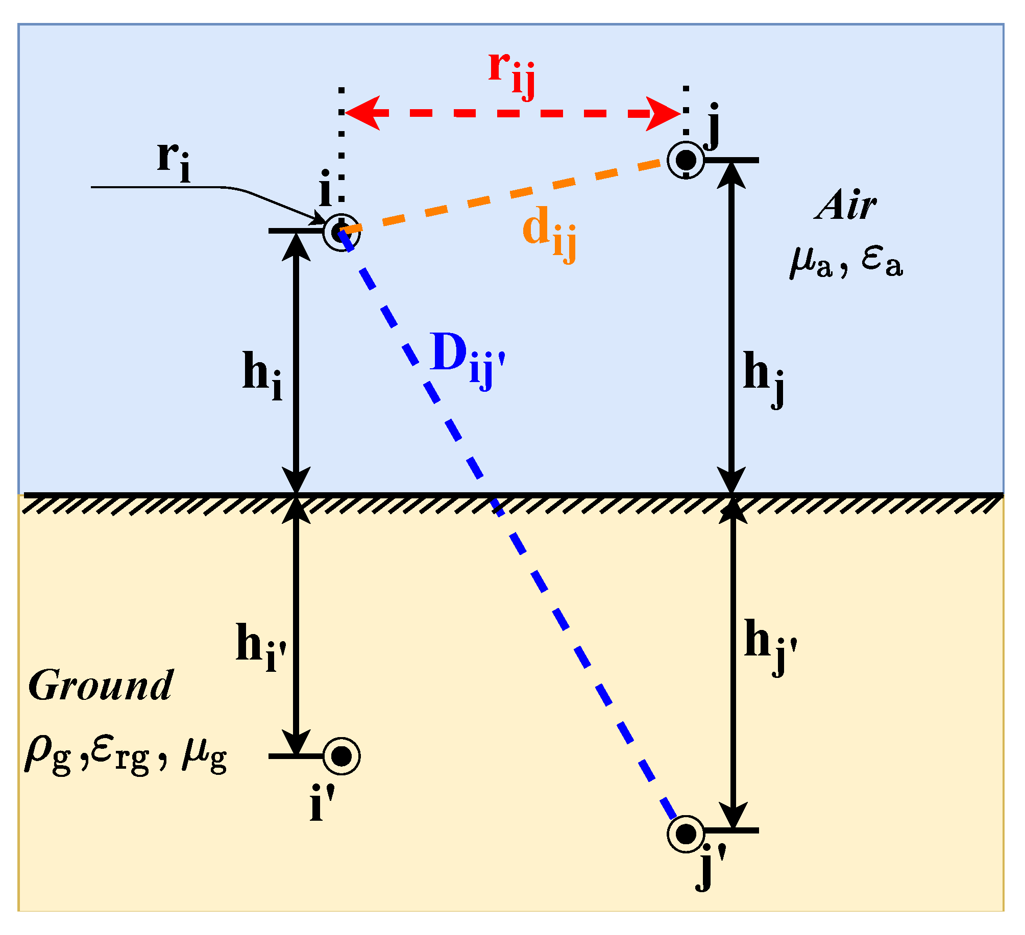
2. Multiphase Overhead Transmission Line Modeling

The Telegrapher’s equations are a pair of differential equations that describe voltages $\left(\mathbf{V}\left(\omega \right)\right)$ and currents $\left(\mathbf{I}\left(\omega \right)\right)$ along the length of a multi-conductor overhead transmission line as follows [26]

$$\frac{\partial \mathbf{V}\left(\omega \right)}{\partial x}=-\mathbf{Z}\left(\omega \right)\mathbf{I}\left(\omega \right),$$

(1)

$$\frac{\partial \mathbf{I}\left(\omega \right)}{\partial x}=-\mathbf{Y}\left(\omega \right)\mathbf{V}\left(\omega \right),$$

(2)

where $\omega =2\pi f$ (rad/s) is the angular frequency and f (Hz) is the frequency. $\mathbf{Z}\left(\omega \right)$ (Ω/m) and $\mathbf{Y}\left(\omega \right)$ (S/m) are the per-unit-length (p.u.l.) longitudinal impedance and transversal admittance matrices of a $(n+1)$-conductor TL.

The longitudinal impedance of a multi-conductor TL depends on the tower geometry, phase geometry, the electromagnetic properties of the medium surrounding these conductors (air and soil), and the frequency [27]. It is given by

$$\mathbf{Z}\left(\omega \right)={\mathbf{Z}}_{\mathrm{int}}\left(\omega \right)+{\mathbf{Z}}_{\mathrm{ext}}\left(\omega \right)+{\mathbf{Z}}_{\mathrm{g}}\left(\omega \right),$$

(3)

where ${\mathbf{Z}}_{\mathrm{int}}\left(\omega \right)$ ($\Omega$/m) is the internal impedance coming from the magnetic field inside the conductor, ${\mathbf{Z}}_{\mathrm{ext}}\left(\omega \right)$ ($\Omega$/m) is the external impedance coming from the magnetic coupling between conductors assuming lossless conductors and lossless ground, and ${\mathbf{Z}}_{\mathrm{g}}\left(\omega \right)$ ($\Omega$/m) is the ground-return impedance that represents the correction factor due to a not perfectly conductive terrain. The p.u.l. transversal admittance of the multi-conductor TL is given by

$$\mathbf{Y}\left(\omega \right)={\left({\mathbf{Y}}_{\mathrm{ext}}^{-1}\left(\omega \right)+{\mathbf{Y}}_{\mathrm{g}}^{-1}\left(\omega \right)\right)}^{-1}=j\omega {\left({\mathbf{P}}_{\mathrm{ext}}+{\mathbf{P}}_{\mathrm{g}}\right)}^{-1},$$

(4)

where ${\mathbf{Y}}_{\mathrm{ext}}\left(\omega \right)$ (S/m) is external admittance and ${\mathbf{Y}}_{\mathrm{g}}\left(\omega \right)$ (S/m) is the ground-return admittance. ${\mathbf{P}}_{\mathrm{ext}}$ (m/F) and ${\mathbf{P}}_{\mathrm{g}}$ (m/F) are the potential coefficients matrices that represent the influence of perfectly conductive and not perfectly conductive ground, respectively. We describe in the following subsections each parcel in (3) and (4).

2.1. Internal Impedance

Internal impedance is due to the Skin effect that appears when a conductor has alternating current passing through its transversal section. As the frequency increases, current concentrates at the conductor’s periphery, causing the conductor’s effective resistance to increase and effective inductance to reduce [28]. Considering a circular conductor, the internal impedance matrix ${\mathbf{Z}}_{\mathrm{int}}\left(\omega \right)$ only contains diagonal elements given by [29]

$${\mathrm{Z}}_{{\mathrm{int}}_{\mathrm{ii}}}\left(\omega \right)=\frac{j{\mathrm{Z}}_{\mathrm{cw}}}{2\pi r_{\mathrm{i}}}\frac{{\mathcal{J}}_0\left(j{\gamma }_{\mathrm{c}}{r}_{\mathrm{i}}\right)}{{\mathcal{J}}_1\left(j{\gamma }_{\mathrm{c}}{r}_{\mathrm{i}}\right)}=-\frac{{\mathrm{Z}}_{\mathrm{cw}}}{2\pi r_{\mathrm{i}}}\frac{{\mathcal{I}}_0\left({\gamma }_{\mathrm{c}}{r}_{\mathrm{i}}\right)}{{\mathcal{I}}_1\left({\gamma }_{\mathrm{c}}{r}_{\mathrm{i}}\right)},$$

(5)

where ${\gamma }_{\mathrm{c}}=\sqrt{j\omega {\mu }_{\mathrm{c}}{\sigma }_{\mathrm{c}}}$ is the propagation constant in the conducting material, and ${\mathrm{Z}}_{\mathrm{cw}}=\sqrt{j\omega {\mu }_{\mathrm{c}}{\sigma }_{\mathrm{c}}^{-1}}$ ($\Omega$/m) is the wave impedance in the conductor. ${\mu }_{\mathrm{c}}={\mu }_{\mathrm{r}}{\mu }_0$ (H/m) is the absolute permeability of the conductor, where ${\mu }_0$ = $4\pi \times {10}^{-7}$ (H/m) is the permeability of free space. ${\mu }_{\mathrm{r}}=1$ for metallic conductors. ${\sigma }_{\mathrm{c}}$ (S/m) is the conductivity of the conductor, $r_{\mathrm{i}}$ (m) is the radius of the conductor, ${\mathcal{J}}_{\mathrm{i}}$ is the Bessel function of first kind of i-th order, and ${\mathcal{I}}_{\mathrm{i}}$ is the modified Bessel function of i-th order. Figure 1 shows a generic configuration of a transmission line in the air-earth media with its conductors and respective images.

2.2. External Impedance

External impedance is the result of time-variant magnetic fields generated by neighboring conductors. The external impedance is a function of the angular frequency, geometry distances, radius and the magnetic permeability of conductor. The elements of the external impedance matrix ${\mathbf{Z}}_{\mathrm{ext}}$$\left(\omega \right)$ are given by [30]

$${\mathrm{Z}}_{{\mathrm{ext}}_{\mathrm{ii}}}\left(\omega \right)=j\omega \frac{{\mu }_0}{2\pi }ln\left(\frac{2h_{\mathrm{i}}}{r_{\mathrm{i}}}\right),$$

(6)

$${\mathrm{Z}}_{{\mathrm{ext}}_{\mathrm{ij}}}\left(\omega \right)=j\omega \frac{{\mu }_0}{2\pi }ln\left(\frac{D_{\mathrm{ij}’}}{d_{\mathrm{ij}}}\right),$$

(7)

where $r_{\mathrm{i}}$ and $h_{\mathrm{i}}$ are the radius and height of conductor i, respectively. $d_{\mathrm{ij}}=\sqrt{r_{\mathrm{ij}}^2+{\left(h_{\mathrm{j}}-h_{\mathrm{i}}\right)}^2}$ is the distance between conductors i and j, $D_{\mathrm{ij}’}=\sqrt{r_{\mathrm{ij}}^2+{\left(h_{\mathrm{j}}+h_{\mathrm{i}}\right)}^2}$ is the distance between conductors i and $j^{\prime }$ (image of j), $h_{\mathrm{j}}$ is the height of conductor j and $r_{\mathrm{ij}}$ is the horizontal distance between the i and j. Figure 1 shows all these geometric variables. All distances are in (m).

2.3. Ground-Return Impedance

In general, TLs transport electric energy from centralized generation facilities to consumers over large distances. Since the TLs are located above lossy grounds, the soil plays a fundamental role in the behavior of voltages and currents along the line. Electromagnetic coupling between conductors and the soil induces Eddy currents in the soil [29].

Several papers model ground by its frequency-constant electrical parameters for homogeneous and stratified media and propose different formulations for the ground-return impedance [31,32,33,34]. In this paper, we consider Carson’s approach [31] and Nakagawa’s formulation [32] to calculate ground-return impedance. In practical applications, the magnetic permeability of the soil ${\mu }_{\mathrm{g}}$ is assumed to be equal to the vacuum magnetic permeability (${\mu }_{\mathrm{g}}$ = ${\mu }_0$${\mu }_{\mathrm{r}}$ (H/m), ${\mu }_{\mathrm{r}}$ = 1).

In 1926, Carson proposed the first model to include the effect of the soil on the longitudinal impedance of TLs [31]. Carson calculates ground impedance by infinite integrals assuming quasi-static electromagnetic field propagation, that the relative permeability of the soil ${\epsilon }_{\mathrm{rg}}=1$, and neglecting the influence of displacement currents in the air and soil [25,31,33,35].

Most available (EMT)-type simulators implement Carson’s formulae to calculate ground-return impedance matrix ${\mathbf{Z}}_{\mathrm{g}}$$\left(\omega \right)$ as follows [31]

$${\mathrm{Z}}_{{\mathrm{g}}_{\mathrm{ii}}}\left(\omega \right)=j\frac{\omega {\mu }_0}{\pi }{\int }_0^{\infty }\frac{e^{-2h_{\mathrm{i}}\lambda }}{\sqrt{{\lambda }^2+j\omega {\mu }_0{\sigma }_{\mathrm{g}}}+\lambda }d\lambda ,$$

(8)

$${\mathrm{Z}}_{{\mathrm{g}}_{\mathrm{ij}}}\left(\omega \right)=j\frac{\omega {\mu }_0}{\pi }{\int }_0^{\infty }\frac{e^{-(h_{\mathrm{i}}+h_{\mathrm{j}})\lambda }}{\sqrt{{\lambda }^2+j\omega {\mu }_0{\sigma }_{\mathrm{g}}}+\lambda }cos\left(r_{\mathrm{ij}}\lambda \right)d\lambda ,$$

(9)

where ${\sigma }_{\mathrm{g}}$ (S/m) is the conductivity of the ground, and $\lambda$ is the integration variable.

In 1948, Wise proposed a solution for calculating the electric field of an infinite conductor parallel to the ground. Wise modeled the soil as a homogeneous semi-infinite plane conductor and considered displacement currents for several relative dielectric permittivities of the soil ${\epsilon }_{\mathrm{rg}}$. Contrary to Wise’s more generic model, Carson’s equations considered ${\epsilon }_{\mathrm{rg}}=1$ [35]. Based on Wise’s equations [36], Nakagawa’s formulae calculate ground-return impedance matrix ${\mathbf{Z}}_{\mathrm{g}}$$\left(\omega \right)$ as follows [32]

$${\mathrm{Z}}_{{\mathrm{g}}_{\mathrm{ii}}}\left(\omega \right)=j\frac{\omega {\mu }_0}{\pi }{\int }_0^{\infty }\frac{e^{-2h_{\mathrm{i}}\lambda }}{{\alpha }_1\frac{{\mu }_0}{{\mu }_{\mathrm{g}}}+\lambda }d\lambda ,$$

(10)

$${\mathrm{Z}}_{{\mathrm{g}}_{\mathrm{ij}}}\left(\omega \right)=j\frac{\omega {\mu }_0}{\pi }{\int }_0^{\infty }\frac{e^{-(h_{\mathrm{i}}+h_{\mathrm{j}})\lambda }}{{\alpha }_1\frac{{\mu }_0}{{\mu }_{\mathrm{g}}}+\lambda }cos\left(r_{\mathrm{ij}}\lambda \right)d\lambda ,$$

(11)

where ${\alpha }_1$ and the squared propagation constants of the air and soil are respectively given by

$${\alpha }_1=\sqrt{{\lambda }^2+{\gamma }_{\mathrm{g}}^2-{\gamma }_{\mathrm{a}}^2},$$

(12)

$${\gamma }_{\mathrm{a}}^2=-{\omega }^2{\mu }_{\mathrm{a}}{\epsilon }_{\mathrm{a}},$$

(13)

$${\gamma }_{\mathrm{g}}^2=j\omega {\mu }_{\mathrm{g}}(j\omega {\epsilon }_{\mathrm{rg}}{\epsilon }_0+{\sigma }_{\mathrm{g}}).$$

(14)

In (12), (13) and (14), the permittivity of air ${\epsilon }_{\mathrm{a}}={\epsilon }_{\mathrm{ra}}{\epsilon }_0$ (F/m) where ${\epsilon }_{\mathrm{a}}$ is the relative permittivity of air, and the permittivity of free space ${\epsilon }_0=8.85\times {10}^{-12}$ (F/m).

2.4. External Admittance

The potential coefficient matrix due to a perfectly conducting ground ${\mathbf{P}}_{\mathrm{ext}}$ in (4) depends solely on the geometric properties of the TL. It contains diagonal and off-diagonal components calculated as follows [30]

$$P_{{\mathrm{ext}}_{\mathrm{ii}}}=\frac{1}{2\pi {ϵ}_0}ln\left(\frac{2h_{\mathrm{i}}}{r_{\mathrm{i}}}\right),$$

(15)

$$P_{{\mathrm{ext}}_{\mathrm{ij}}}=\frac{1}{2\pi {ϵ}_0}ln\left(\frac{D_{\mathrm{ij}’}}{d_{\mathrm{ij}}}\right).$$

(16)

From (15) and (16), the external admittance matrix

$${\mathbf{Y}}_{\mathrm{ext}}\left(\omega \right)=j\omega {\mathbf{P}}_{\mathrm{ext}}^{-1}.$$

(17)

2.5. Ground-Return Admittance

Based on Wise’s work [36], Nakagawa proposed in [32] the elements of the potential coefficient matrix ${\mathbf{P}}_{\mathrm{g}}$ in (4) as follows

$$P_{{\mathrm{g}}_{\mathrm{ii}}}=\frac{1}{\pi {\epsilon }_0}{\int }_0^{\infty }\frac{\left(\lambda +\frac{{\mu }_{\mathrm{g}}}{{\mu }_0}{\alpha }_1\right)e^{-2h_{\mathrm{i}}\lambda }}{\left(\lambda +\frac{{\mu }_0}{{\mu }_{\mathrm{g}}}{\alpha }_1\right)\left(\frac{\lambda {\gamma }_{\mathrm{g}}^2}{{\gamma }_{\mathrm{a}}^2}+{\alpha }_1\right)}d\lambda ,$$

(18)

$$P_{{\mathrm{g}}_{\mathrm{ij}}}=\frac{1}{\pi {\epsilon }_0}{\int }_0^{\infty }\frac{\left(\lambda +\frac{{\mu }_{\mathrm{g}}}{{\mu }_0}{\alpha }_1\right)e^{-(h_{\mathrm{i}}+h_{\mathrm{j}})\lambda }}{\left(\lambda +\frac{{\mu }_0}{{\mu }_{\mathrm{g}}}{\alpha }_1\right)\left(\frac{\lambda {\gamma }_{\mathrm{g}}^2}{{\gamma }_{\mathrm{a}}^2}+{\alpha }_1\right)}cos\left(r_{\mathrm{ij}}\lambda \right)d\lambda ,$$

(19)

which results in the not perfectly conductive ground admittance

$${\mathbf{Y}}_{\mathrm{g}}\left(\omega \right)=j\omega {\mathbf{P}}_{\mathrm{g}}^{-1}.$$

(20)

Equations (12)–(14) defines ${\alpha }_1$, the propagation constants of the air ${\gamma }_{\mathrm{a}}^2$ and soil ${\gamma }_{\mathrm{g}}^2$.

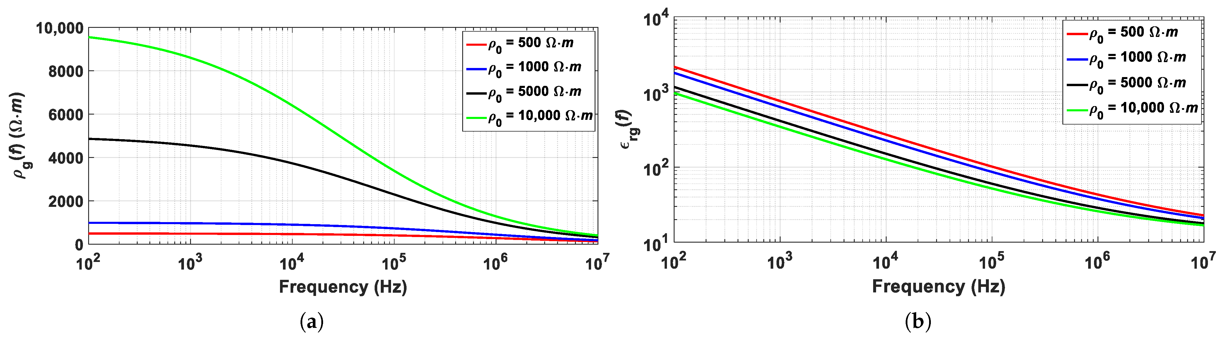
3. Frequency-Dependent Soil Electrical Parameters

Soils consist of a very complex composition of compacted layers of earth made of organic and inorganic materials and rock that have disintegrated. The electrical soil parameters are dependent on the frequency and on the environmental factors such as the temperature, humidity and size of soil particles [24]. The electromagnetic properties that characterize a soil are the magnetic permeability ${\mu }_{\mathrm{g}}$, resistivity ${\rho }_{\mathrm{g}}$ (or conductivity ${\sigma }_{\mathrm{g}}={\rho }_{\mathrm{g}}^{-1}$), and absolute dielectric permittivity ${\epsilon }_{\mathrm{rg}}$. The magnetic permeability is practically frequency independent and assumed to be equal to vacuum ${\mu }_{\mathrm{g}}={\mu }_0$. However, the last two, ${\rho }_{\mathrm{g}}$ and ${\epsilon }_{\mathrm{rg}}$, are greatly affected by the frequency specially for high-resistive soils [37,38,39].

Based on the frequency-domain Ampere–Maxwell’s law, the total electric current density $\overrightarrow{J_{\mathrm{T}}}$ (A/m²) in a dielectric medium when an external electrical field $\overrightarrow{E}$ (V/m) is applied is give by [15]

$$\nabla \times \overrightarrow{H}=\overrightarrow{J_{\mathrm{T}}}=\overrightarrow{J_{\mathrm{c}}}+\overrightarrow{J_{\mathrm{D}}}={\sigma }_0\overrightarrow{E}+j\omega {\epsilon }_{\mathrm{rg}}\overrightarrow{E},$$

(21)

where $\overrightarrow{H}$ (A/m) is the magnetic field, $\overrightarrow{J_{\mathrm{c}}}$ and $\overrightarrow{J_D}$ (A/m²) are conductive and capacitive currents densities. The ${\sigma }_0$ (S/m) is the low-frequency conductivity, considered as a real number associated to the transport of electric charge and losses generated to the in the conducting process. However, the dielectric permittivity is a complex number which can be written as ${\epsilon }_{\mathrm{rg}}={\epsilon }_{\mathrm{rg}}^{\prime }-j{\epsilon }_{\mathrm{rg}}^{″}$, where ${\epsilon }_{rg}^{\prime }$ is related to the ability of the material to be polarized and store energy whereas ${\epsilon }_{\mathrm{rg}}^{\prime \prime }$ represents the losses generated due to the heat generated by the dipole frictions in the several polarization processes as detailed in [15,40]. Inserting $\epsilon$ in (21), yields

$$\nabla \times \overrightarrow{H}=\left({\sigma }_0+\omega {\epsilon }_{\mathrm{rg}}^{\prime \prime }\right)\overrightarrow{E}+j\omega {\epsilon }_{\mathrm{rg}}^{\prime }\overrightarrow{E}=\left({\sigma }_{\mathrm{eff}}+j\omega {\epsilon }_{\mathrm{rg}}^{\prime }\right)\overrightarrow{E}.$$

(22)

As shown by this equation, the effective conductivity ${\sigma }_{\mathrm{eff}}$ (S/m) increases with the frequency whereas the ${\epsilon }_{\mathrm{rg}}^{\prime }$ decreases as the frequency of the applied field increases as detailed in [40]. The physical explanation related to the electric resistivity ${\rho }_{\mathrm{g}}$ and dielectric permittivity ${\epsilon }_{\mathrm{rg}}$, and the different polarization processes that occurs in the ground molecules are explained in [41].

As the frequency increases, the polarization processes are not able to follow the fast alternations of the electric field. This causes ${\epsilon }_{\mathrm{rg}}^{\prime }$ to decrease as frequency increases. However, at high frequencies, there is an increase of losses per cycle causing ${\epsilon }_{\mathrm{rg}}^{″}$ to increase its value. From these variations, as the frequency increases, the value of ${\sigma }_{\mathrm{eff}}$ increases while the value of ${\epsilon }_{\mathrm{eff}}$ decreases. In [41], Friedman thoroughly explains the polarization processes of ground molecules that affect electric resistivity ${\rho }_{\mathrm{g}}$ and dielectric permittivity ${\epsilon }_{\mathrm{rg}}$.

In the 1930s, Smith carried out the first study regarding frequency dependence of soil electrical parameters [42]. Later, in the 1970s, several authors developed theoretical and experimental models based on field experiments as summarized in [5,16]. Recently, in the electromagnetic software tools that solve the frequency-domain Maxwell’s equations include the frequency dependence of soil electrical parameters to carry out the lightning performance on grounding systems and on transmission lines such as in [22,37,38,39,43].

Based on field measurements of different soils in Brazil, Visacro and Alípio proposed curve-fitted expressions to calculate the frequency dependence of soil resistivity ${\rho }_{\mathrm{g}}$ and relative permittivity ${\epsilon }_{\mathrm{rg}}$ as a function of frequency [14]. Later, in 2014, they presented a semi-theoretical causal model to obtain frequency-dependent soil electrical parameters based on various measurements in the 100 Hz–4 MHz frequency range.

Alípio and Visacro’s model adopts three levels of conservativeness to take the dispersion of the frequency dependence of the soil and eventual uncertainties into account. This model proposes the following equations [15]

$${\rho }_{\mathrm{g}}\left(f\right)={\sigma }_0^{-1}{\left[1+h\left({\sigma }_0\right){\left(\frac{f}{1MHz}\right)}^{\xi }\right]}^{-1},$$

(23)

$${\epsilon }_{\mathrm{rg}}\left(f\right)=\frac{{\epsilon }_{\infty }^{\prime }}{{\epsilon }_0}+{\sigma }_0\frac{tan(\pi \xi /2)\times {10}^{-3}}{2\pi {\epsilon }_0{\left(1MHz\right)}^{\xi }}h\left({\sigma }_0\right)f^{\xi -1},$$

(24)

where ${\sigma }_0$ (mS/m) is the low-frequency (at 100 Hz) conductivity of the soil and ${\epsilon }_{\infty }^{\prime }/{\epsilon }_0$ is the relative permittivity at higher frequencies. The values employed in this simulation for $h\left({\sigma }_0\right)$, $\xi$, and ${\epsilon }_{\infty }^{\prime }/{\epsilon }_0$ are: $h\left({\sigma }_0\right)$ = 1.26 ${\sigma }_0^{-0.73}$, $\xi$ = 0.54 and ${\epsilon }_{\infty }^{\prime }/{\epsilon }_0$ = 12 [15].

To show the impact of frequency in the soil electrical parameters, we calculated the electrical parameters of soils with low, medium, and high resistivity from 100 Hz to 10 MHz using (23) and (24). Figure 2 shows the resistivity ${\rho }_{\mathrm{g}}$ and relative permittivity ${\epsilon }_{\mathrm{rg}}$ of soils that have a 100 Hz resistivity ${\rho }_0$ of 500, 1000, 5000, and 10,000 Ω·m which are related to several types of soil according to [16].

Figure 2 shows that high resistivity soils (${\rho }_0)$ = 5000 and 10,000 Ω·m are much more affected by the frequency effect than soils with moderate and low resistivity. As ${\rho }_0$ increases, the relative permittivity ε_rg decreases asymptotically to values between 15 and 30 (typical values of soils represented by frequency-independent parameters). The soils of 500, 1000, 5000 and 10,000 Ω·m will be considered in the transient analysis of this work. Another reason for choosing high resistive soils is based on the recent works considering the same resistive range in their works [21,22,23].

According to CIGRE [16], practical engineering studies or EMT analysis of TLs involving the lightning performance of grounding systems buried on soils with resistivity above of 700 Ω·m must consider the frequency dependence of ${\rho }_{\mathrm{g}}$ and ${\epsilon }_{\mathrm{rg}}$. For transmission lines, the CIGRE brochure [16] recommends that lines located on soils of resistivity above 700 Ω·m, the frequency dependence of the soil must be considered for a precise transient analysis. The recommendations about considering the frequency dependence of the soil for studies on transmission lines are summarized as follows [16].

• $\rho$ < 300 Ω·m, the recommendation is to ignore the frequency-dependency of soil;
• 300 ≤ $\rho$ < 700 Ω·m, it is recommended to include the frequency-dependency of soil;
• $\rho$ ≥ 700 Ω·m, it is mandatory to consider the frequency-dependency of soil for a precise transient analysis.

4. Lightning Modeling

Lightning is one of the primary sources of outages in electrical power systems due to the back flashover mechanism and other insulation failures that can occur in several pieces of equipment [34]. In this context, lately, several authors had worked on the lightning performance of overhead multiphase transmission lines [22,44,45], wind turbines [43,46] and renewable-based hybrid systems [47,48].

Lightning current waveforms contain frequency components from DC to a few tens of MHz [30,49]. Therefore, for accurate computation of transient responses on power systems, ground-return impedance and admittance must consider the frequency dependence of soil electrical parameters [49].

To assess the impact of frequency-dependent soil models on the transient responses of overhead TLs, we evaluate the overvoltages caused by two different high-frequency waveforms: Subsequent return stroke and Gaussian pulse. We consider the Heidler’s function to represent the subsequent return stroke because is a widely mathematical expression that represents the lightning currents which provide more realistic results [47,50]. Gaussian function are employed due to its larger frequency content and this type of function is usually used to show the performance of time-domain response of the models [51].

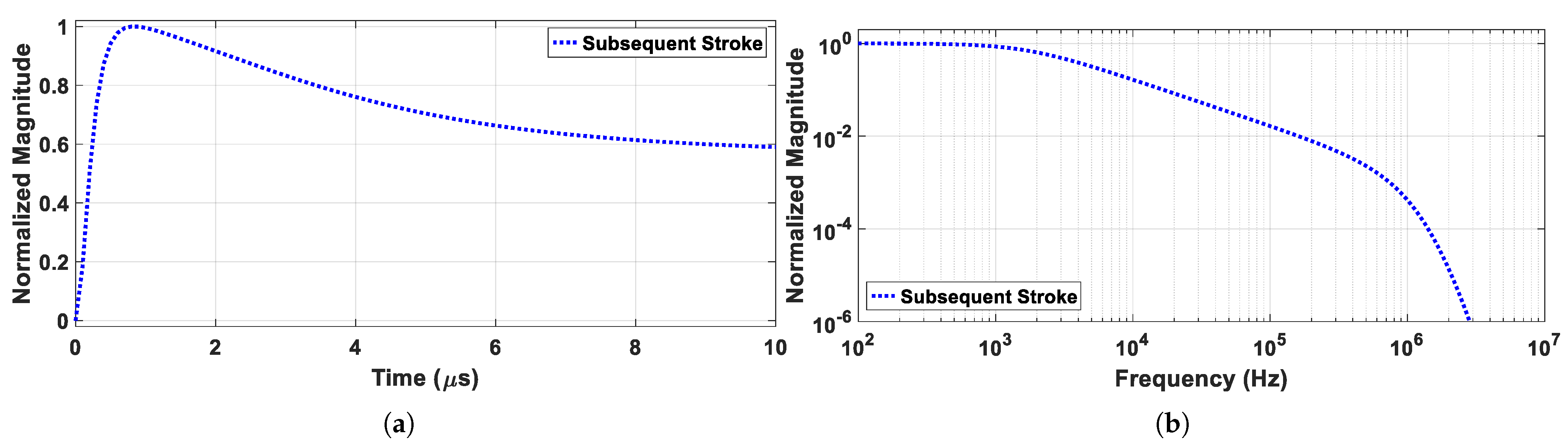
4.1. Subsequent Return Stroke

The subsequent return stroke current is characterized by a peak value of 12 kA and a virtual front time of 0.67 μs, which is defined as the time between 30% and 90% of its peak value divided by 0.6, and the time-to-half-peak of 50 μs as detailed in [45,46]. Heidler’s function models a subsequent return stroke as follows [46,52]

$$I\left(t\right)=\sum _{n=1}^N\frac{I_{0i}}{{\eta }_{\mathrm{i}}}\frac{{(t/{\tau }_{1\mathrm{i}})}^{n_{\mathrm{i}}}}{1+{(t/{\tau }_{1\mathrm{i}})}^{n_{\mathrm{i}}}}{e}^{-t/{\tau }_{2\mathrm{i}}},$$

(25)

$${\eta }_{\mathrm{i}}=exp{\left[-\left(\frac{{\tau }_{1\mathrm{i}}}{{\tau }_{2\mathrm{i}}}\right)\left(n_{\mathrm{i}}\frac{{\tau }_{2\mathrm{i}}}{{\tau }_{1\mathrm{i}}}\right)\right]}^{1/n},$$

(26)

where $I_{0\mathrm{i}}$ (A) is the peak value of the current. ${\tau }_{1\mathrm{i}}$ and ${\tau }_{2\mathrm{i}}$ (s) are the front and decay times of the i-th Heidler function, respectively. $n_{\mathrm{i}}$ is an integer coefficient, and $\eta$ is a correction factor to adjust the peak.

In this paper, we use the subsequent return stroke current waveform to perform time-domain simulations. We model the subsequent return stroke waveform $I\left(t\right)$ as a sum of two Heidler functions $I_1\left(t\right)+I_2\left(t\right)$, where the peak value of the current $I_{\mathrm{p}}$ is 12.09 kA. The parameters for both Heidler functions $I_1$ and $I_2$ are presented in

Table 1. Parameters for lightning subsequent stroke current.

Impulsive Current	${\mathit{I}}_0$ (kA)	${\mathit{\tau }}_1$(μs)	${\mathit{\tau }}_2$(μs)	n	η	${\mathit{I}}_{\mathbf{p}}$ (kA)
Subsequent stroke ($I_1$)	10.7	0.25	2.5	2	0.6394	12.09
Subsequent stroke ($I_2$)	6.5	2.1	230	2	0.8765

. $I\left(t\right)$ has a maximum steepness (current derivative) of 40 kA/μs [52].

We present the normalized subsequent return stroke waveform and its normalized 100 Hz–10 MHz frequency spectrum in Figure 3.

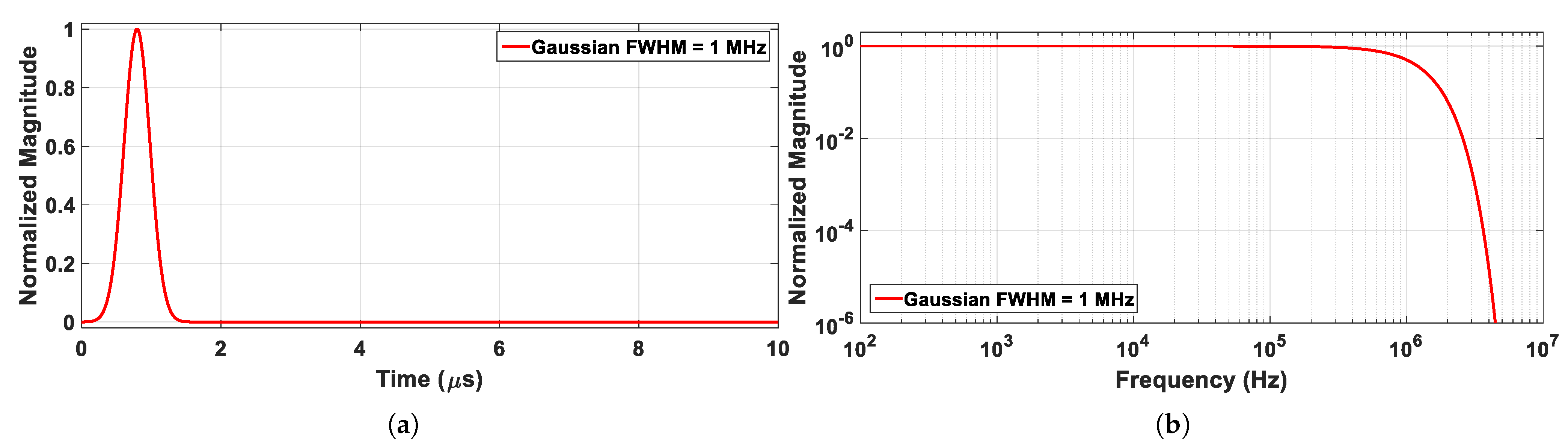
4.2. Gaussian Pulse

In this paper, we investigate the impact of frequency-dependent soil parameters on the TL parameters, which ultimately affect the time-domain response of the TL. For this purpose, we employ waveforms that contain high-frequency components such as the Gaussian pulse, which is given by

$$I\left(t\right)=I_{0}exp\left[-{\left(\frac{\beta }{{\tau }_0}\right)}^2{\left(t-{\tau }_0\right)}^2\right],$$

(27)

where ${\tau }_0$ (s) is the delay time, $\beta$ is a coefficient, and $I_0$ (A) is the peak of the current.

Table 2. Parameters of a Gaussian pulse that has a FWHM of 1 MHz.

Impulsive Current	${\mathit{I}}_0$ (kA)	${\mathit{\tau }}_0$ (ns)	$\mathit{\beta }$
Gaussian Pulse	1.6	440	1.1774

shows the parameters of a 1 MHz full width at half maximum (FWHM) Gaussian pulse.

Figure 4 portrays a normalized 1 MHz–FWHM Gaussian pulse in the time domain and its normalized frequency-domain counterpart.

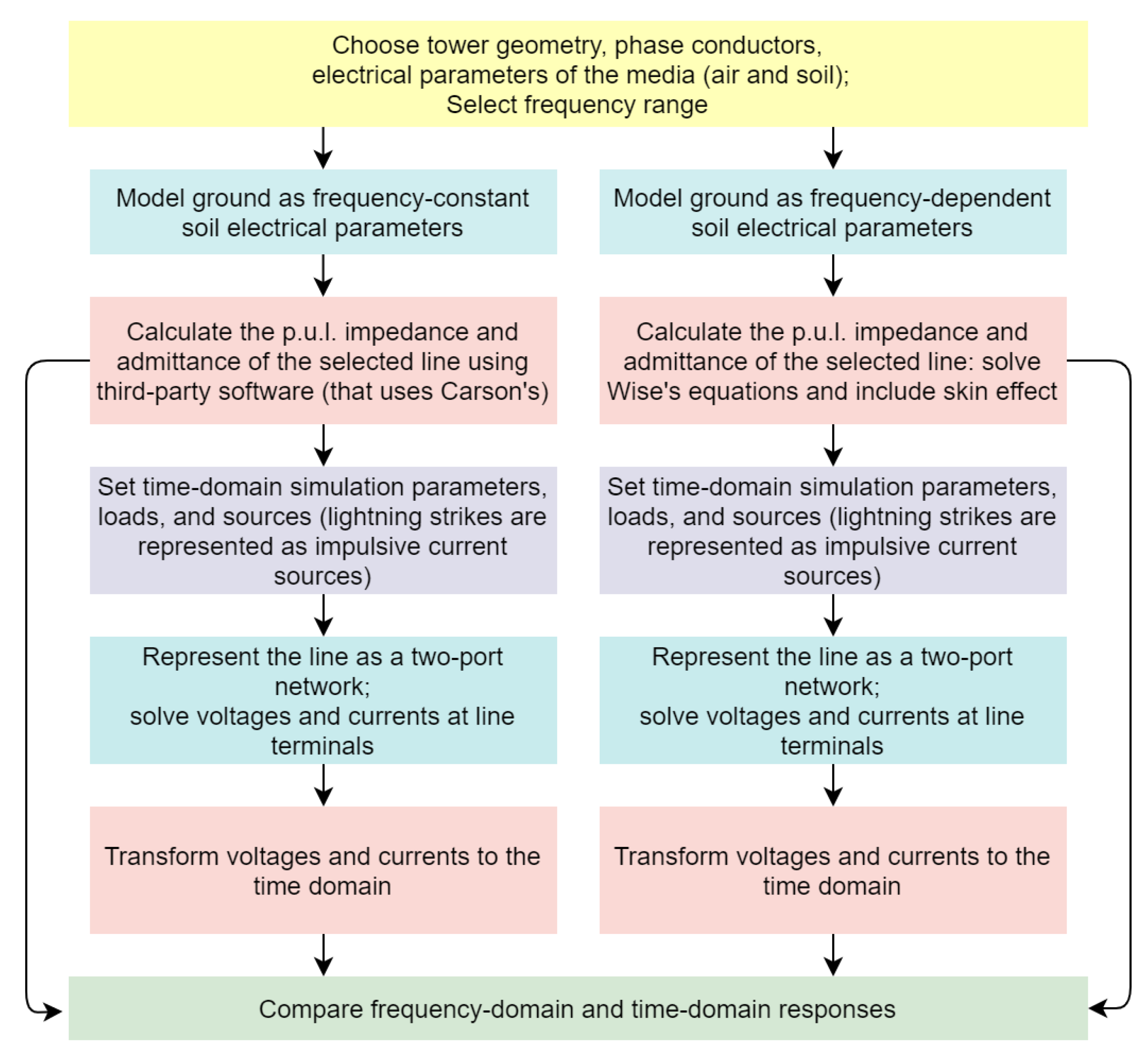
5. Methodology

The methodology for compute the frequency- and time-domain responses are presented in this section. In our analysis, we disregard the tower surge impedance, tower-footing grounding electrodes and the ionization of the soil. Figure 5 shows the steps performed to obtain frequency and time-domain results, which are summarized as follows:

Step 1: Define transmission line configuration: Tower geometry and conductor parameters such as bundle and radius of the phase and ground wires conductors. Choose the electrical parameters (conductivity, relative permittivity, and magnetic permeability) of air and soil. Select the frequency range, varying from 100 Hz up to 10 MHz. To include the frequency dependence of soil parameters, we calculate the frequency-dependent relative permittivity and conductivity of the soil from the soil conductivity measured at 100 Hz using (23) and (24) [15].

Step 2: Use (3) and (4) to calculate the p.u.l. impedance matrix $\mathbf{Z}\left(\omega \right)$ and p.u.l. admittance matrix $\mathbf{Y}\left(\omega \right)$ of the TL defined in Step 1. This paper compares:

• the parameters computed by MatLab using the powersys/power_lineparam routine, that uses Carson’s Equations (8) and (9). In this Matlab tool, the ground-return admittance ${\mathbf{Y}}_{\mathrm{g}}\left(\omega \right)$ is neglected, resulting in ${\mathbf{Y}}_{\mathrm{t}}\left(\omega \right)$ = ${\mathbf{Y}}_{\mathrm{ext}}\left(\omega \right)$. Furthermore, the Carson’s approach considers that the soil is modeled by frequency-independent parameters and the displacement currents are ignored.
• the parameters calculated using Nakagawa’s formulae, where ${\mathbf{Z}}_{\mathrm{int}}\left(\omega \right)$, ${\mathbf{Z}}_{\mathrm{ext}}\left(\omega \right)$, ${\mathbf{Z}}_{\mathrm{g}}\left(\omega \right)$, ${\mathbf{Y}}_{\mathrm{ext}}\left(\omega \right)$, ${\mathbf{Y}}_{\mathrm{g}}\left(\omega \right)$ are respectively given by (5), (6), (7), (10), (11), (17) and (20). We use Alípio’s Equation (23) and (24) to include the frequency dependence of ${\rho }_{\mathrm{g}}$ and ${\epsilon }_{\mathrm{rg}}$.

Step 3: Define simulation parameters e.g., time step, simulation time. Select the type of lightning strike waveform connected to the TL. In this paper, we model lightning strikes as ideal current sources that contain the waveforms presented in Section 4. Set the loads connected to the receiving end (open-circuit, short-circuit or load).

Step 4: Calculate the line’s two-port equations (y-parameters) that relate terminals’ currents to voltages using the line parameters calculated in step 2. The two-port equations are described in [53]. Compute voltages and currents at line terminals in the frequency domain.

Step 5: Transform voltages and currents to the time domain using the Numerical Laplace Transform [54]. Then, we compare the time-domain responses.

All the calculations are carried out in MatLab.

6. Numerical Results and Discussion

We present our results in three sections:

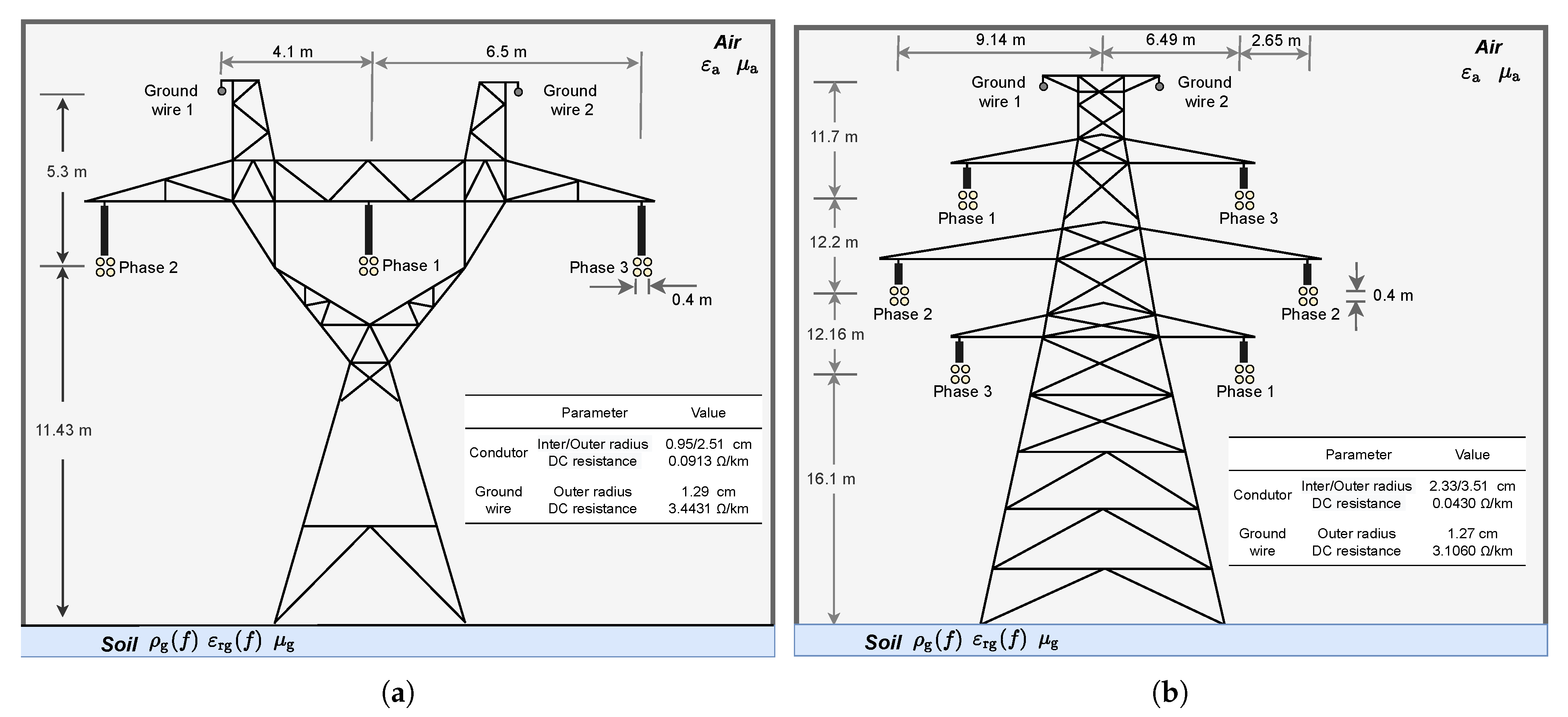
• Section 6.1 shows the longitudinal impedance and transversal admittance of a single-circuit three-phase TL and a double-circuit three-phase TL, including the ground wires at the top, located above four homogeneous soils.
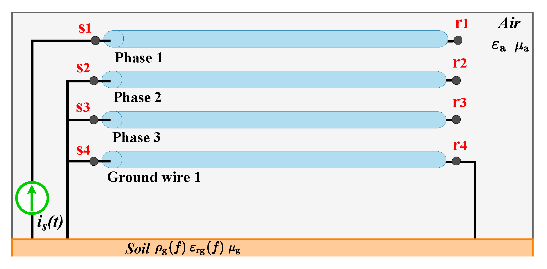
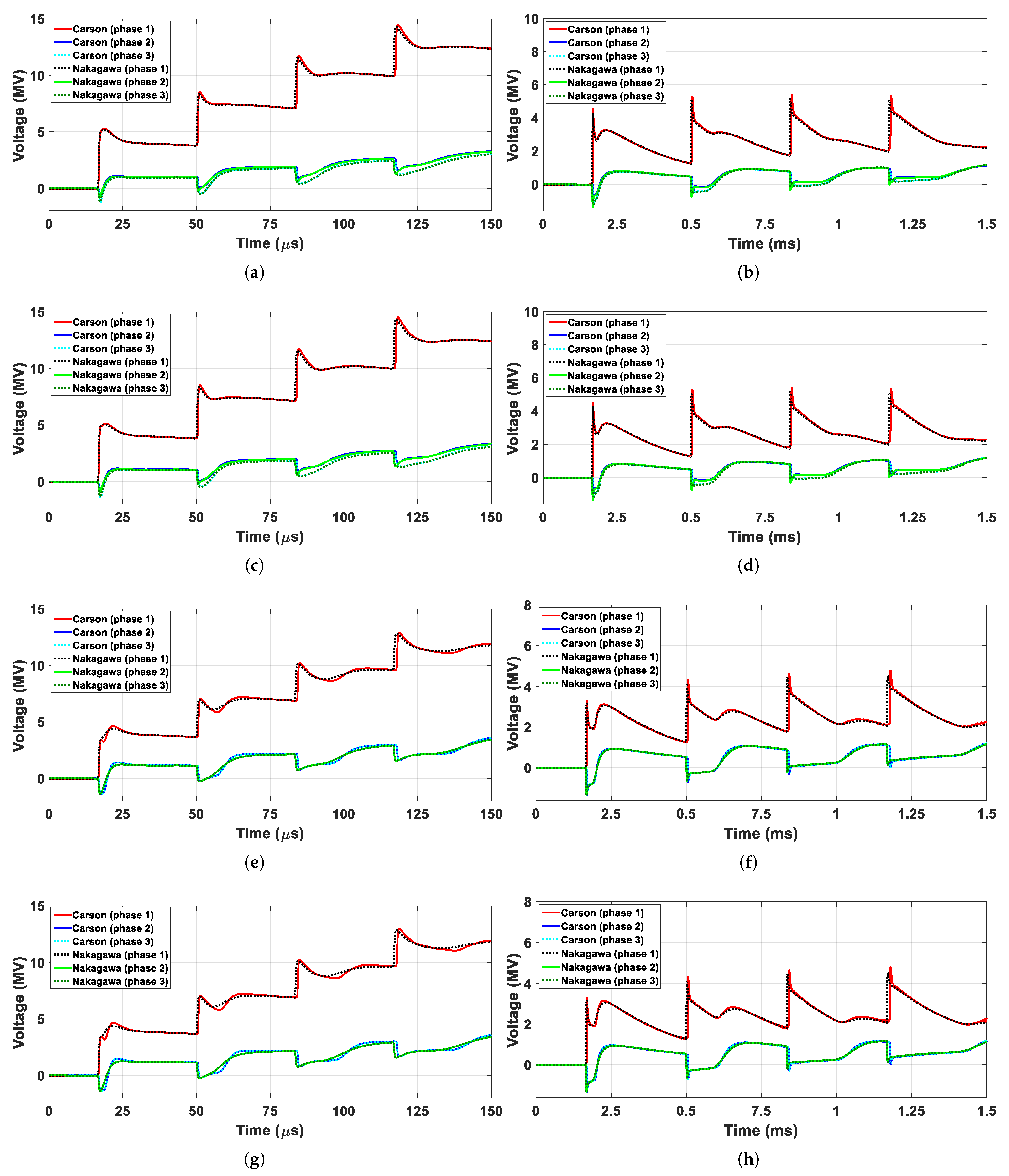
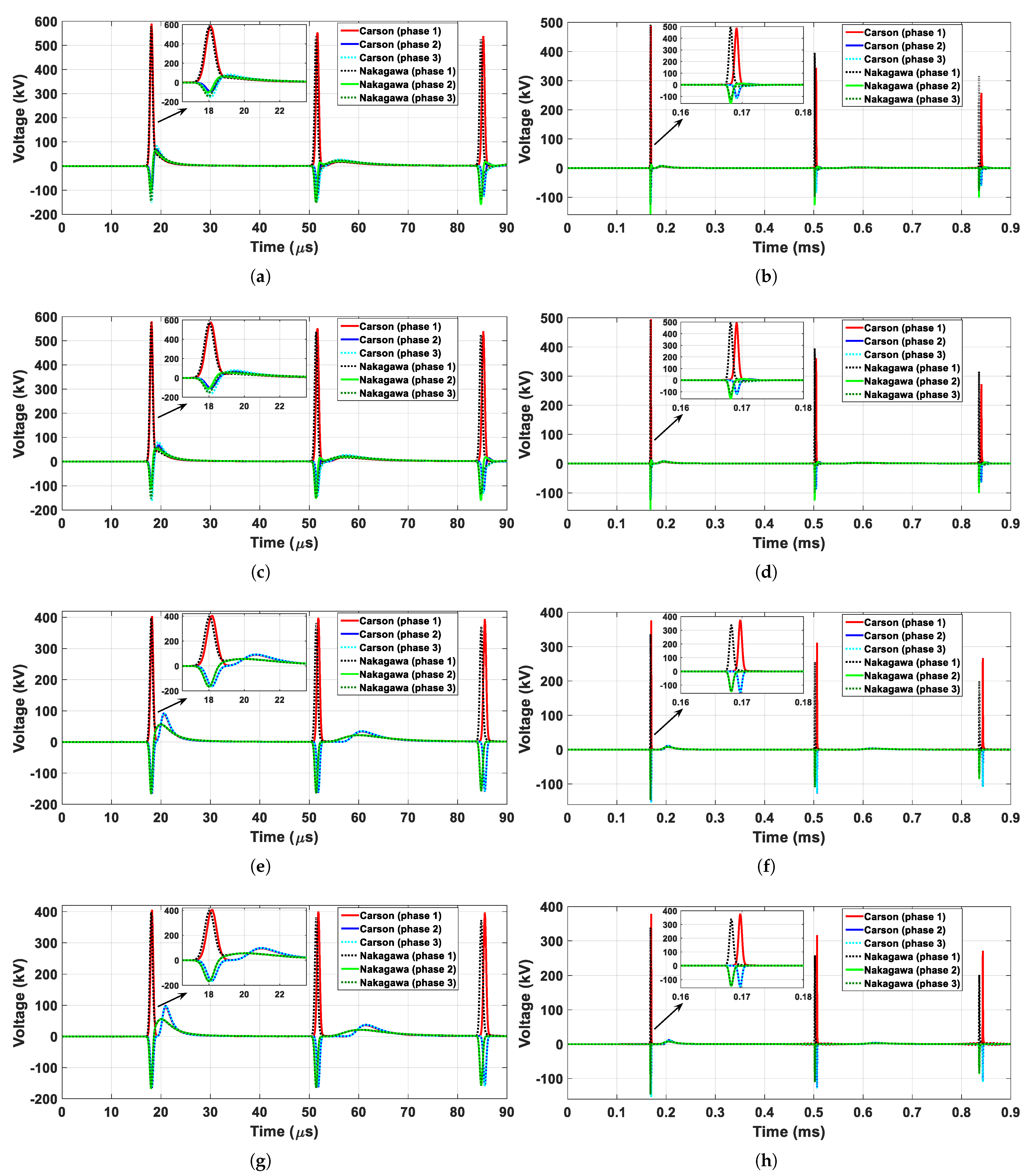
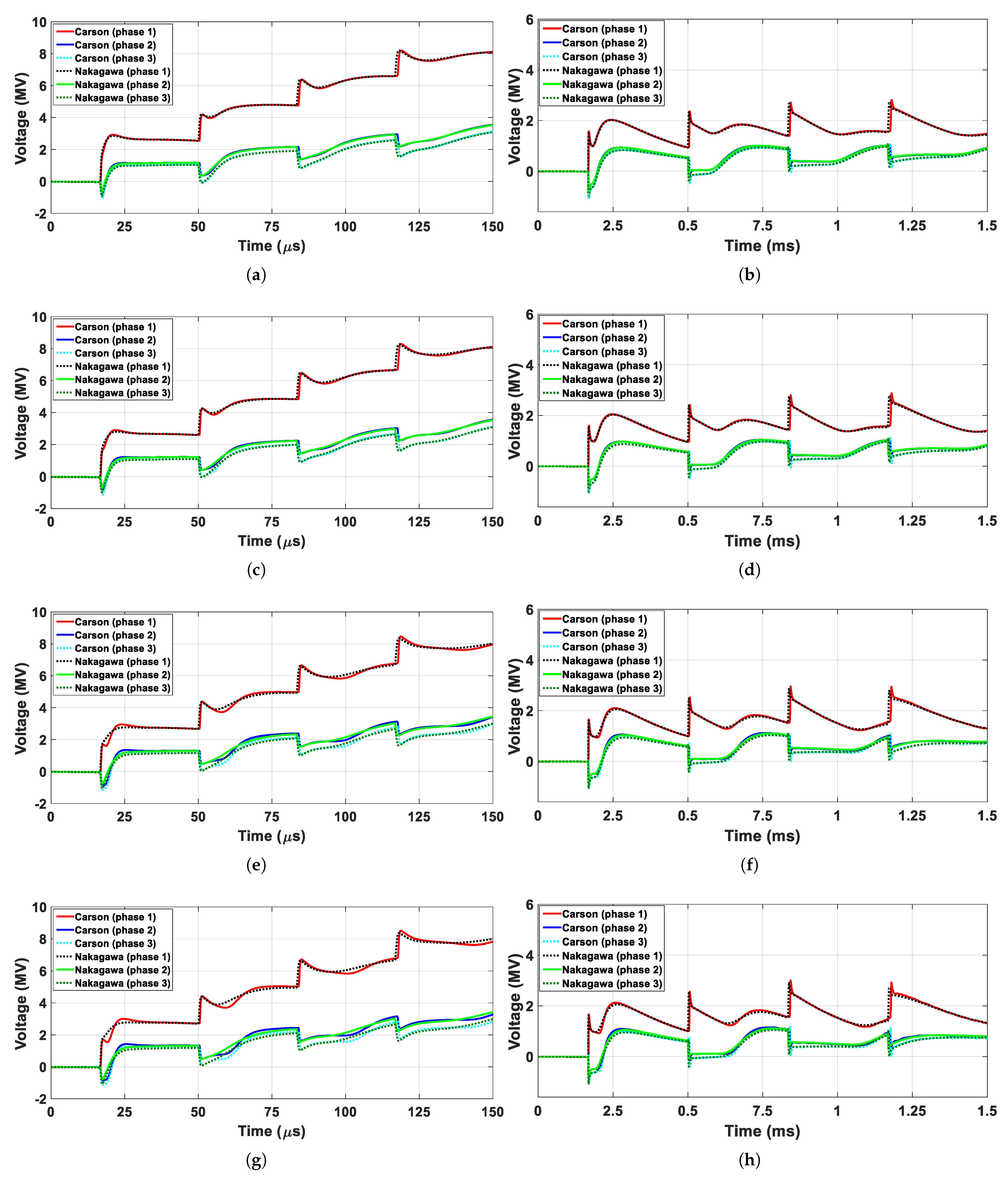
• Section 6.2 shows the transient responses of the single-circuit three-phase TL with ground wires subject to lightning currents modeled as the subsequent return stroke of Section 4.1 and the Gaussian pulse of Section 4.2.
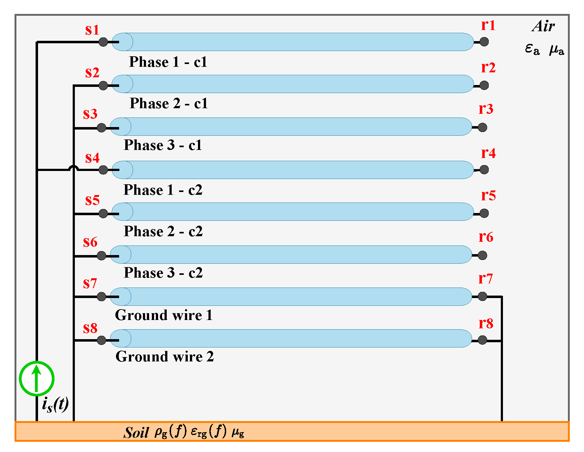
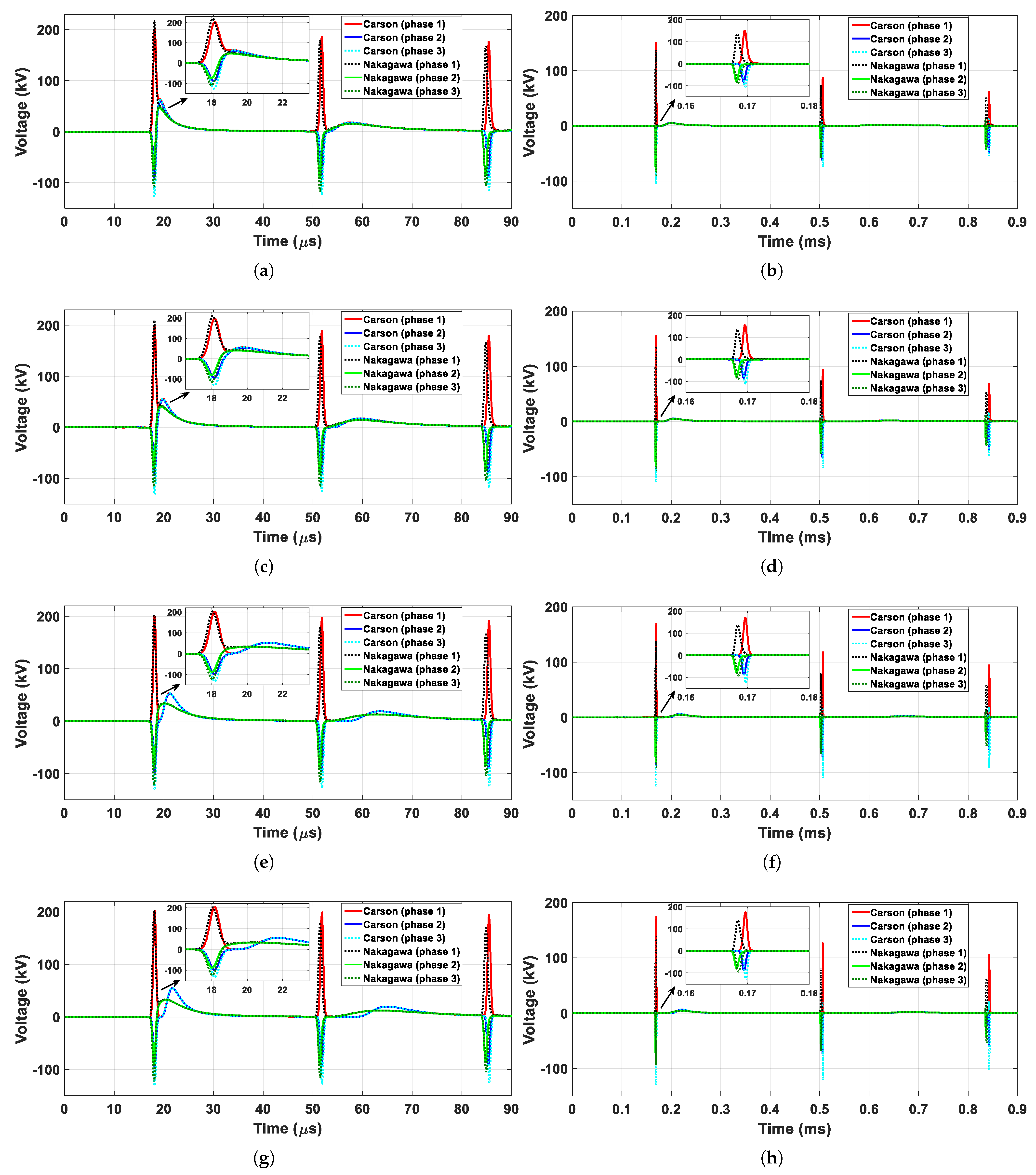
• Section 6.3 shows the transient responses of the double-circuit three-phase TL with ground wires, subject to lightning currents modeled as the subsequent return stroke of Section 4.1 and the Gaussian pulse of Section 4.2.

We computed the transient responses of the single-circuit three-phase TL of Figure 6a and the double-circuit three-phase TL of Figure 6b. We considered two line lengths: 5 km and 50 km. Both TLs are located above four types of homogeneous high-resistive soils that have a 100 Hz resistivity of 500 Ω·m, 1000 Ω·m, 5000 Ω·m and 10,000 Ω·m.

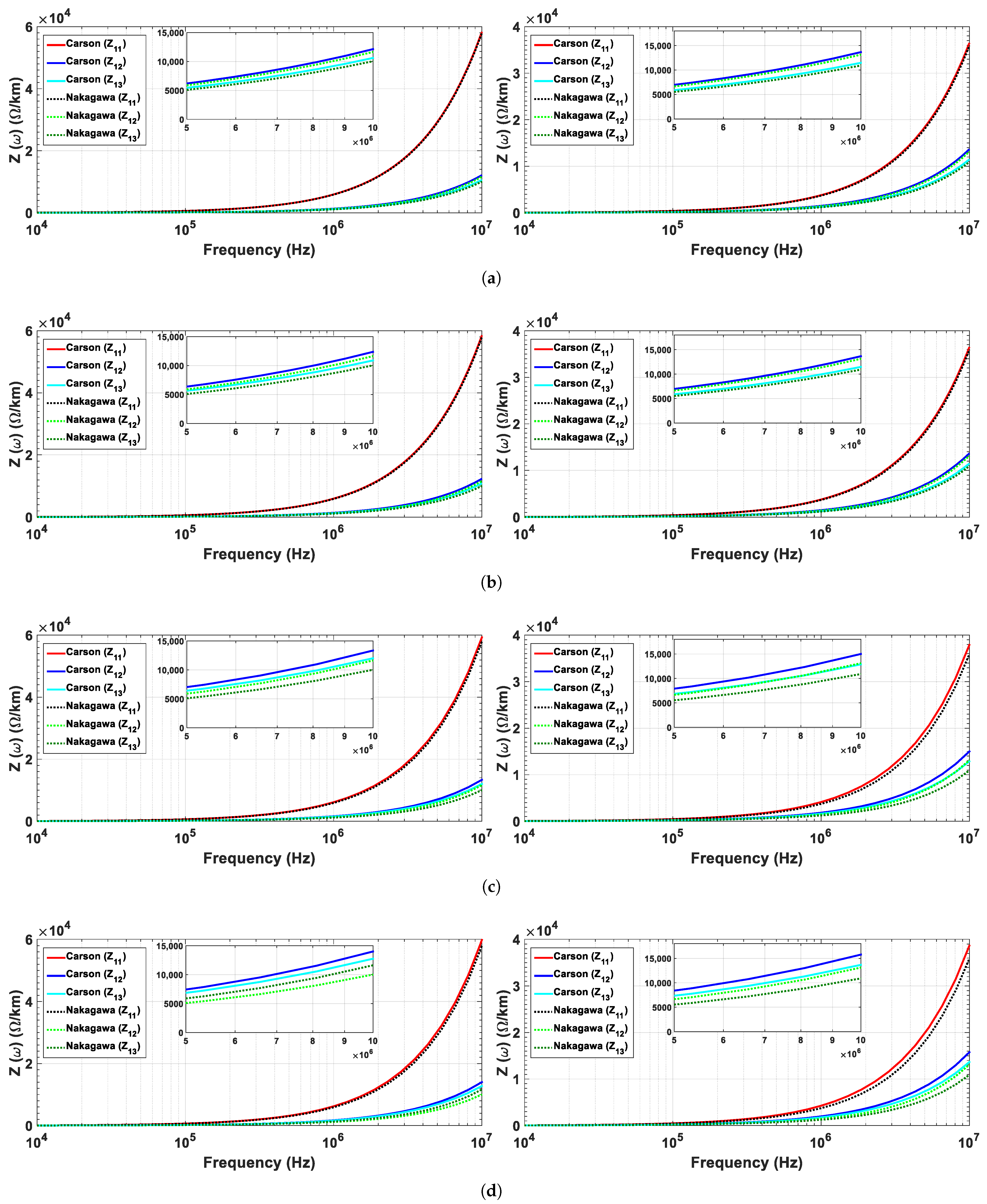
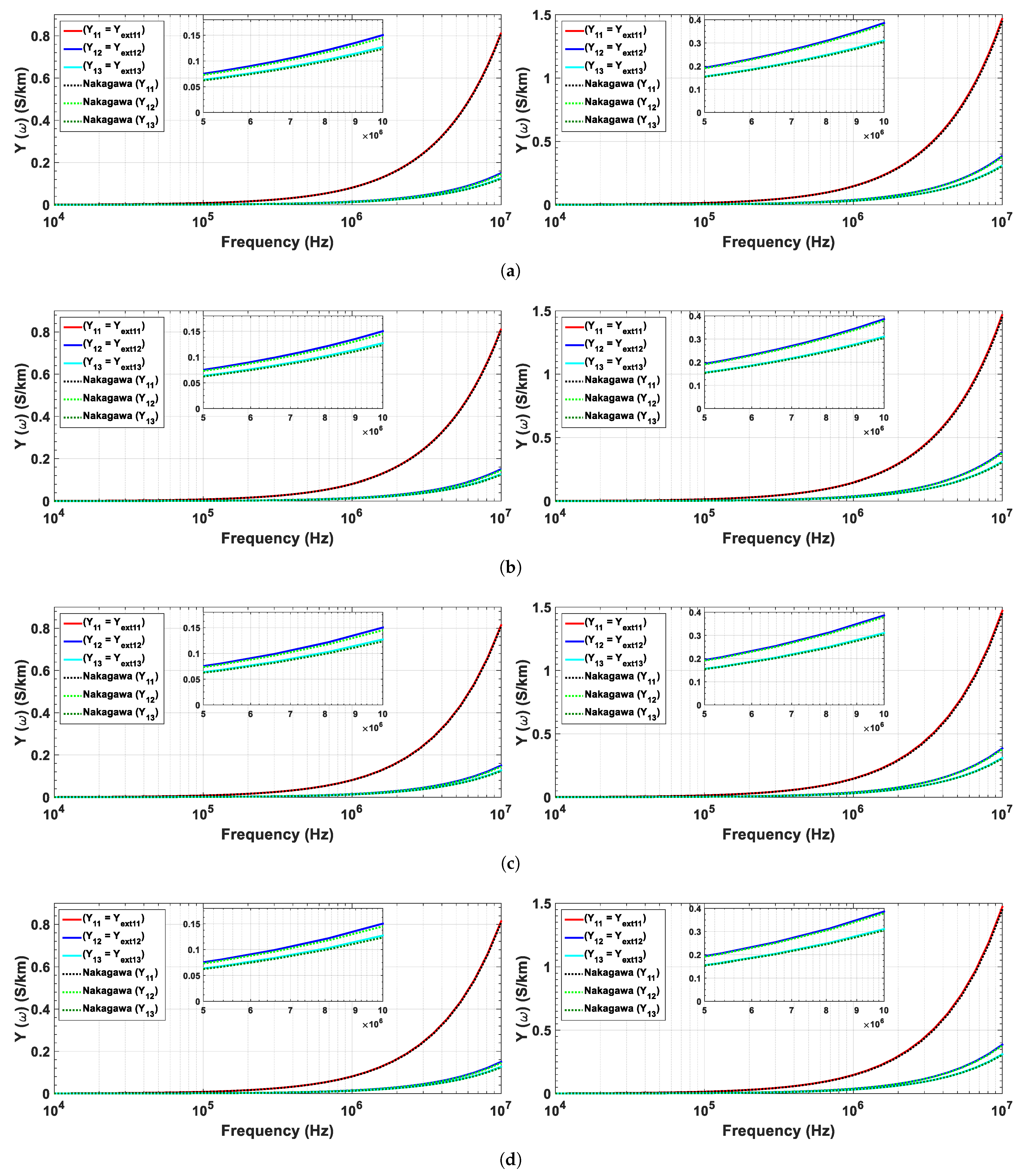
6.1. Longitudinal Impedance and Transversal Admittance

We computed the longitudinal impedance and transversal admittance matrices of the single-circuit three-phase TL of Figure 6a and the double-circuit three-phase TL of Figure 6b, both with ground wires at the top of the towers, using the following approaches:

• Carson’s approach–frequency constant soil parameters: Equations (5)–(7) allow the calculation of the internal and external impedances in (3). MatLab’s powersys/power_lineparam routine estimates the ground-return impedance by solving Carson’s Formula (8) and (9) considering frequency-constant resistivities of 500 Ω·m, 1000 Ω·m, 5000 Ω·m and 10,000 Ω·m. Carson’s approach considers the soil as a perfect conductor for the calculation of the shunt admittance. This approach neglects the displacement currents dispersed in the ground. Therefore ${\mathbf{Y}}_{\mathrm{g}}\left(\omega \right)$ is neglected ($\mathbf{Y}\left(\omega \right)$ = ${\mathbf{Y}}_{\mathrm{ext}}\left(\omega \right)$).
• Nakagawa’s approach—frequency dependent soil parameters: Equations (5)–(7) allow the calculation of the internal and external impedances in (3). Nakagawa’s Formulae (10), (11), (18) and (19) in combination with Alípio and Visacro’s Equation (23) and (24) allow the calculation of ${\mathbf{Z}}_{\mathrm{g}}\left(\omega \right)$ and ${\mathbf{Y}}_{\mathrm{g}}\left(\omega \right)$ matrices considering frequency-dependent soil electrical parameters. The frequency-dependent soil resistivity ${\sigma }_{\mathrm{g}}\left(f\right)$ and permittivity ${\epsilon }_{\mathrm{rg}}\left(f\right)$ are computed for soils that have a 100 Hz resistivity of 500 Ω·m, 1000 Ω·m, 5000 Ω·m and 10,000 Ω·m.

For both approaches, we compare in Figure 7 and Figure 8 the elements in the first row of $\mathbf{Z}\left(\omega \right)$ and $\mathbf{Y}\left(\omega \right)$, respectively. We chose to show only the elements in the first row of each matrix because $\mathbf{Z}\left(\omega \right)$ and $\mathbf{Y}\left(\omega \right)$ are symmetrical. To better show the differences in the magnitudes of $\mathbf{Z}\left(\omega \right)$ and $\mathbf{Y}\left(\omega \right)$, results presented in Figure 7 and Figure 8 are calculated for the 10 kHz–10MHz frequency range.

Figure 7 shows that ${\mathrm{Z}}_{11}$, ${\mathrm{Z}}_{12}$, and ${\mathrm{Z}}_{13}$ increase rapidly after 200 kHz. At 10 MHz, ${\mathrm{Z}}_{11}$ reaches a value of 60,000 Ω/km for the single-circuit TL and 40,000 Ω/km for the double-circuit TL. Carson’s approach estimates higher values than Nakagawa’s approach with frequency-dependent soil resistivity and relative permittivity. This occurs because Carson’s formula neglects displacement currents by assuming that the relative permittivity of the soil is equal to 1, a constant value in a quasi-static transverse electromagnetic mode.

On the other hand, Nakagawa’s approach includes the frequency-dependent soil relative permittivity in the propagation function ${\gamma }_{\mathrm{g}}$ in (14). For both TLs, the low-frequency resistivity did not cause significant differences on ${\mathrm{Z}}_{11}$, ${\mathrm{Z}}_{12}$, and ${\mathrm{Z}}_{13}$. As can be seen, for the soils of 500 Ω·m and 1000 Ω·m, they present similar values for the elements ${\mathrm{Z}}_{11}$, ${\mathrm{Z}}_{12}$, and ${\mathrm{Z}}_{13}$ in all frequency range. However, as the frequency increases, the difference between the two approach are pronounced for the ${\mathrm{Z}}_{11}$, ${\mathrm{Z}}_{12}$, and ${\mathrm{Z}}_{13}$ computed for the 5000 Ω·m and 10,000 Ω·m. The difference is more significant for the double-circuit transmission line. The difference between the values occur due to higher variation in the soil resistivity as the frequency increases which is more pronounced for high resistive soils, as seen in the Figure 2.

Figure 8 shows that the transversal admittance also increases rapidly after 200 kHz. Carson’s approach neglects ${\mathbf{Y}}_{\mathrm{g}}\left(\omega \right)$, whereas Nakagawa’s approach includes the frequency-dependent soil electrical parameters in the calculation of ${\mathbf{Y}}_{\mathrm{g}}\left(\omega \right)$. However, Figure 8 shows that both approaches generate similar admittances, which means that ${\mathbf{Y}}_{\mathrm{g}}\left(\omega \right)$ does not affect $\mathbf{Y}\left(\omega \right)$ substantially. In addition, note that variation of ${\rho }_0$ has almost no effect in the calculation of $\mathbf{Y}\left(\omega \right)$. The maximum value of the transversal admittance element Y₁₁ for the double-circuit transmission line reaches approximately 1.5 S/km, whereas for the single-circuit line, the admittance element Y₁₁ is equal to 0.8 S/km.

We observe that both approaches have lead to similar results for transversal admittance and the frequency dependence of the soil parameters has no significant impact on these elements Y₁₁, Y₁₂, and Y₁₃.

Based on the behavior of the ground-return impedances and admittances, the time-domain transient responses on transmission lines located above high-resistive soils are influenced by fast-front disturbances such as the lightning discharges, characterized by high-frequency spectrum as detailed in the following sections.

6.2. Single-Circuit Transmission Line

We place the single-circuit three-phase TL with ground wires of Figure 6a located above four high-resistive soils, each having a resistivity of 500 (Ω·m), 1,000 (Ω·m), 5000 (Ω·m) and 10,000 (Ω·m). Figure 7 and Figure 8 show the p.u.l. longitudinal impedance and transversal admittance of each of these lines, calculated using Carson’s approach and Nakagawa’s approach, respectively. For each soil, we consider TL with lengths of 5 km and 50 km. We leave one of the line terminals open-circuited and connect the other terminal to two distinct current sources, detailed as follows:

• the subsequent return stroke of Section 4.1, and
• the 1-MHz FWHM Gaussian pulse of Section 4.2,

as shown in Figure 9. Figure 10 and Figure 11 depict the transient voltages in each of these scenarios according to

Table 3. Simulation results for the single-circuit three-phase TL of Figure 9.

Lightning Current	Soil Resistivity (Ω·m)	TL Length
		5 km	50 km
Subsequent stroke	500	Figure 10a	Figure 10b
	1000	Figure 10c	Figure 10d
	5000	Figure 10e	Figure 10f
	10,000	Figure 10g	Figure 10h
Gaussian Pulse	500	Figure 11a	Figure 11b
	1000	Figure 11c	Figure 11d
	5000	Figure 11e	Figure 11f
	10,000	Figure 11g	Figure 11h

.

Figure 10 and Figure 11 contain several voltage peaks caused by reflections from the receiving end due to traveling waves within the TL. The line’s open-circuited terminal causes voltage peaks to be more intense. The number and intensity of each reflection depend on the lightning current waveform and the length of the TL. For instance, the 5 km TL has more intense voltage peaks than the line that is 50 km long. The short duration of the Gaussian pulses causes their reflections to be more distinguishable from each other. Figure 10 and Figure 11 also show shift between time-domain responses that increases with time. This behaviour can be seen in the detailed in Figure 11.

In order to investigate the diffenreces in the time-domain responses, we present in

Table 4. Percentage deviation for the transient voltages on the phase-1 generated on the single-circuit line located on the high-resistive soils.

Peaks	LT length	Soil Resistivity (Ω·m)	Subsequent Stroke	Gaussian Pulse
First peak	5 km	500	1.59	1.50
		1000	1.61	0.99
		5000	5.47	1.41
		10,000	6.26	1.75
	50 km	500	6.01	−0.57
		1000	5.39	−0.70
		5000	3.77	10.72
		10,000	3.91	10.74
Second peak	5 km	500	2.49	2.71
		1000	2.08	2.25
		5000	0.82	4.19
		10,000	0.89	4.32
	50 km	500	4.97	−14.89
		1000	4.90	−9.39
		5000	4.26	18.07
		10,000	4.31	18.65
Third peak	5 km	500	1.70	2.46
		1000	1.36	2.53
		5000	0.49	5.97
		10,000	0.58	6.12
	50 km	500	4.69	−24.09
		1000	4.68	−15.66
		5000	4.42	26.15
		10,000	4.43	25.83

the percent deviation between voltage peaks simulated considering frequency-dependent soil parameters (FD-Nakagawa’s Approach) and frequency-independent soil parameters (FI-Carson’s approach). The percentage deviation is calculated in the following equation

$$\delta =\frac{V_{\mathrm{p}}^{FI}-V_{\mathrm{p}}^{FD}}{V_{\mathrm{p}}^{FI}}\times 100\%,$$

(28)

where the voltage peak $V_{\mathrm{p}}$ is obtained considering the frequency-independent (FI) or the frequency-dependent soil model (FD). We calculate the percent deviation between the first three peaks for each simulation.

Table 4 shows that the deviation is more pronounced in the simulations where the lightning current source is represented by the 1MHz - FWHM Gaussian pulse of Section 4.2.

The maximum percent deviation is 26.15% which is obtained between the Carson’s approach and Nakagawa’s approach for the third peak for the 50 km single-circuit TL located soil of 5000 Ω·m generated by the Gaussian pulse. This difference occurs to due the attenuation constant is higher frequencies associated with Carson’s approach is larger than that calculated by the Nakagawa’s approach. However, for the 50 km single-circuit TL located soils of 500 Ω·m and 1000 Ω·m, the percentage deviation is negative associated to the Gaussian pulse. This occur due to the larger frequency content of the Gaussian pulse associated with soils of moderate resistivity.

The difference between the voltage peaks for the Carson’s approach with frequency-independent and Nakagawa’s approach with frequency-dependent soil models are more pronounced for those computed by the Gaussian pulse due to its higher energy at the high frequencies compared to subsequent return stroke.

6.3. Double-Circuit Transmission Line

Similar to the single-circuit TL, we place the double-circuit three-phase TL including the ground wires of Figure 6b above four high-resistive soils, each having a resistivity of 500 Ω·m, 1000 Ω·m, 5000 Ω·m and 10,000 Ω·m. Figure 7 and Figure 8 show, respectively, the p.u.l. longitudinal impedance and transversal admittance of each of these lines calculated using Carson’s approach and Nakagawa’s approach. For each soil, we considered two line lengths: 5 km and 50 km. We leave one of the line terminals open-circuited and connect the other terminal to a subsequent return stroke waveform and a 1 MHz—FWHM Gaussian pulse.

We present in:

• Table 5. Simulation results for the double-circuit three-phase TL of Figure 12.

  Lightning Current	Soil Resistivity (Ω·m)	TL Length
  		5 km	50 km
  Subsequent stroke	500	Figure 13a	Figure 13b
  	1000	Figure 13c	Figure 13d
  	5000	Figure 13e	Figure 13f
  	10,000	Figure 13g	Figure 13h
  Gaussian Pulse	500	Figure 14a	Figure 14b
  	1000	Figure 14c	Figure 14d
  	5000	Figure 14e	Figure 14f
  	10,000	Figure 14g	Figure 14h

  the plots obtained for each simulation,
• Figure 12 the circuit employed for the simulations,
• Figure 13 and Figure 14 the transient voltages at the receiving end of the TL for each of the scenarios mentioned above,
• Table 6. Percentage deviation for the transient voltages on the phase-1 generated on the double-circuit line located on the high-resistive soils.

  Peaks	LT Length	Soil Resistivity (Ω·m)	Subsequent Stroke	Gaussian Pulse
  First peak	5 km	500	2.43	−7.00
  		1000	3.41	−6.12
  		5000	6.53	−0.98
  		10,000	7.75	−0.24
  	50 km	500	1.20	8.93
  		1000	1.74	13.36
  		5000	2.33	19.67
  		10,000	2.34	21.09
  Second peak	5 km	500	−0.14	3.42
  		1000	−0.02	5.62
  		5000	0.34	9.45
  		10,000	0.54	10.48
  	50 km	500	0.93	16.95
  		1000	1.48	21.99
  		5000	2.05	33.82
  		10,000	2.14	36.75
  Third peak	5 km	500	−0.10	4.74
  		1000	0.03	6.84
  		5000	0.64	12.34
  		10,000	1.11	13.27
  	50 km	500	1.14	18.60
  		1000	1.43	24.53
  		5000	2.22	39.15
  		10,000	2.52	42.75

  the voltage peak deviation between Carson’s approach (frequency-constant soil parameters) and Nakagawa’s approach (frequency-dependent soil parameters).

Similar to the single-circuit TL, the percentage deviation is higher for the simulations that include the Gaussian pulse.

The percentage deviation increases with the length of the line, reaching a maximum value of 42.75% in the third peak of the double-circuit line that is located above a 10,000 Ω·mm soil. Furthermore, the percentage deviation of voltage peaks is more pronounced for the double circuit TL than those computed for the single-circuit TL using the Gaussian pulse. The electromagnetic coupling between conductors causes the induced voltages of phases 2 and 3, which have significant amplitudes. The frequency dependence of soil parameters also has an impact on the voltage peaks in phases 2 and 3 where can present a significant difference between the two approaches.

The percentage deviations increase as the soil resistivity increases for the voltages on the double-circuit transmission lines for both types of lightning currents as seen in the Table 6. The first peaks of the transient responses calculated by Nakagawa’s approach is slightly higher than those computed by Carson’s approach, using the Gaussian pulse on the 5 km double-circuit line. The difference in voltage peaks calculated with both approaches increases with soil resistivity. This difference is also dependent on the type of lightning current which affects significantly in the reduction of the voltage peaks. It is demonstrated that when the frequency dependence of the soil is considered, this reduction can be around 42% for the double-circuit line above the 10,000 Ω·mm soil subject to the Gaussian pulse. This result can be explained due to the fact that the Gaussian pulse contains a large frequency content associated with high energy im comparison with the subsequent stroke.

Results demonstrated that accurate computation of electromagnetic transients requires the proper modeling of the soil. In that case, the frequency-dependent soil electrical parameters must be included to compute the ground-return impedance and admittance of the transmission lines. The importance in the calculation of accurate responses results in the correct sizing of insulation for many components in power systems, e.g., insulator strings, pre-insertion resistors, surge arresters, and transformers [30,55]. By an accurate evaluation of voltage peaks, insulation can be estimated more accurately and thus reduce costs.

Inaccurate estimation of voltage peaks could result in malfunctions of the protective devices, inadequate installation of the surge arrester in lines that can lead to outages in power systems while degrading the quality of supplied energy. Furthermore, most of the available Electromagnetic transient (EMT)-type simulators compute the ground impedance using Carson’s approach which can result in high errors when the transmission line is located above high-resistive soils. This paper highlights the importance of combining the Nakagawa’s approach to the computation of the ground-return impedance and ground-return admittance including the frequency-dependent soil parameters.

7. Conclusions

The main objective of this paper was to investigate the frequency- and time-domain transient responses of single and double-circuit multiphase transmission lines (including the ground wires at the top of these towers) located above soils of moderate and high resistive values. It was demonstrated that the frequency effect has a significant impact on the soil electrical parameters (resistivity and permittivity) especially for soils of high resistivity.

For this purpose, the ground was represented by well established frequency-dependent soil model proposed by Alípio and Visacro where the ground-return impedances and admittances were computed for this type of soil using the Nakagawa’s approach. On the other hand, the same parameters were computed using the Carson’s approach which assumes frequency-constant soil parameters. It is demonstrated that the longitudinal impedance and transversal admittance present a pronounce deviations at the high frequencies, especially for the high-resistive soils. Some elements of ground-return impedance and ground-return admittance matrices were calculated for Carson’s approach and compared with Nakagawa’s approach for high resistive soils. Results indicated that the proper and mutual elements present distinct values at the high frequencies which the difference between the two approaches increases as the soil resistivity increases. As a consequence, the impact of the frequency effect on time-domain responses on single and -double circuit transmission lines generated by two fast-front disturbances (lightning strikes) hitting the upper phases is assessed. The transient voltages at the receiving ends are dependent of the lightning current waveform, soil electrical parameters and the line parameters such as the tower configuration and the line length. The peak values of the transient voltages computed for the Nakagawa’s approach are lower than those assessed by Carson’s approach. The lightning current modeled by the Gaussian pulse has provided the more significant percentage deviations for the transmission lines analysed. Reductions of 26.15% and 42.75% are found in the voltage peaks of the single- and double-circuit transmission lines, respectively. These significant reductions are due to the larger frequency spectrum of the Gaussian pulse in comparison with the spectrum of the subsequent return stroke. This deviation is more pronounced as the line lengths increase for transmission lines located on high resistive soils. As the main contribution of this paper, we provided that the frequency dependence of the soil electrical parameters must be taken into account in the ground-return parameters for transmission line modeling. Proper soil modeling must be included in the (EMT)-type simulators to carry out precise transient analysis in a power system.

References

- Silveira, F.H.; Visacro, S.; Alipio, R.; De Conti, A. Lightning-induced voltages over lossy ground: The effect of frequency dependence of electrical parameters of soil. IEEE Trans. Electromagn. Compat. 2014, 56, 1129–1136. [Google Scholar] [CrossRef]
- Visacro, S.; Silveira, F.H. The impact of the frequency dependence of soil parameters on the lightning performance of transmission lines. IEEE Trans. Electromagn. Compat. 2015, 57, 434–441. [Google Scholar] [CrossRef]
- Pascoalato, T.; de Araújo, A.; Kurokawa, S.; Pissolato Filho, J. Analysis of transient voltages and currents in short transmission lines on frequency-dependent soils. Electr. Power Syst. Res. 2021, 194, 107103. [Google Scholar] [CrossRef]
- Salarieh, B.; Kordi, B. Full-wave black-box transmission line tower model for the assessment of lightning backflashover. Electr. Power Syst. Res. 2021, 199, 107399. [Google Scholar] [CrossRef]
- Cavka, D.; Mora, N.; Rachidi, F. A comparison of frequency-dependent soil models: Application to the analysis of grounding systems. IEEE Trans. Electromagn. Compat. 2013, 56, 177–187. [Google Scholar] [CrossRef]
- Ratcliffe, J.; White, F. LXIII. The electrical properties of the soil at radio frequencies. Lond. Edinb. Dublin Philos. Mag. J. Sci. 1930, 10, 667–680. [Google Scholar] [CrossRef]
- Smith-Rose, R. The electrical properties of soil for alternating currents at radio frequencies. Proc. R. Soc. Lond. Ser. Contain. Pap. Math. Phys. Character 1933, 140, 359–377. [Google Scholar]
- Scott, J.; Carroll, R.; Cunningham, D. Dielectric Constant and Electrical Conductivity of Moist Rock from Laboratory Measurements. US Dept. of Interior Geological Survey Technical Letter, Special Projects-12. August 1964; Volume 17. Available online: http://ece-research.unm.edu/summa/notes/SSN/note116.pdf (accessed on 17 August 2021).
- Longmire, C.L.; Smith, K.S. A Universal Impedance for Soils; Technical Report; Mission Research Corp.: Santa Barbara, CA, USA, 1975; Available online: https://apps.dtic.mil/sti/pdfs/ADA025759.pdf (accessed on 17 August 2021).
- Messier, M. The Propagation of an Electromagnetic Impulse through Soil: Influence of Frequency Dependent Parameters; Technical Report MRC-N-415; Mission Research Corp.: Santa Barbara, CA, USA, 1980. [Google Scholar]
- Visacro, S.; Portela, C. Soil permittivity and conductivity behavior on frequency range of transient phenomena in electric power systems. In Proceedings of the International Symposium on High Voltage Engineering, Stadthalle, Germany, 24–28 August 1987. [Google Scholar]
- Portela, C. Measurement and modeling of soil electromagnetic behavior. In Proceedings of the IEEE International Symposium on Electromagnetic Compatability, Seattle, WA, USA, 2–6 August 1999; Volume 2, pp. 1004–1009. [Google Scholar]
- Visacro, S.; Alipio, R.; Vale, M.H.M.; Pereira, C. The response of grounding electrodes to lightning currents: The effect of frequency-dependent soil resistivity and permittivity. IEEE Trans. Electromagn. Compat. 2011, 53, 401–406. [Google Scholar] [CrossRef]
- Visacro, S.; Alipio, R. Frequency dependence of soil parameters: Experimental results, predicting formula and influence on the lightning response of grounding electrodes. IEEE Trans. Power Deliv. 2012, 27, 927–935. [Google Scholar] [CrossRef]
- Alipio, R.; Visacro, S. Modeling the frequency dependence of electrical parameters of soil. IEEE Trans. Electromagn. Compat. 2014, 56, 1163–1171. [Google Scholar] [CrossRef]
- Cigré, W.G. Impact of Soil-Parameter Frequency Dependence on the Response of Grounding Electrodes and on the Lightning Performance of Electrical Systems (C4.33). Technical Brochure 781. 2019. Available online: https://e-cigre.org/publication/781-impact-of-soil-parameter-frequency-dependence-on-the-response-of-grounding-electrodes-and-on-the-lightning-performance-of-electrical-systems (accessed on 17 August 2021).
- Wedepohl, L.; Efthymiadis, A.E. Wave propagation in transmission lines over lossy ground: A new, complete field solution. Proc. Inst. Electr. Eng. 1978, 125, 505–510. [Google Scholar] [CrossRef]
- De Lima, A.C.S.; Portela, C.M. Inclusion of frequency-dependent soil parameters in transmission-line modeling. IEEE Trans. Power Deliv. 2007, 22, 492–499. [Google Scholar] [CrossRef]
- Gertrudes, J.B.; Tavares, M.C.; Portela, C. Transient analysis on overhead transmission line considering the frequency dependent soil representation. In Proceedings of the 2011 IEEE Electrical Power and Energy Conference, Detroit, MI, USA, 24–28 July 2011; pp. 362–367. [Google Scholar] [CrossRef]
- Portela, C.M.; Tavares, M.C.; Filho, J.P. Accurate representation of soil behaviour for transient studies. IEE Proc. Gener. Transm. Distrib. 2003, 150, 736–744. [Google Scholar] [CrossRef]
- De Conti, A.; Emídio, M.P.S. Simulation of transients with a modal-domain based transmission line model considering ground as a dispersive medium. In Proceedings of the IPST’2015—International Conference on Power Systems Transients, Cavtat, Croatia, 15–18 June 2015. [Google Scholar]
- De Conti, A.; Emídio, M.P.S. Extension of a modal-domain transmission line model to include frequency-dependent ground parameters. Electr. Power Syst. Res. 2016, 138, 120–130. [Google Scholar] [CrossRef]
- Moura, R.A.; Schroeder, M.A.; Menezes, P.H.; Nascimento, L.C.; Lobato, A.T. Influence of the soil and frequency effects to evaluate atmospheric overvoltages in overhead transmission lines—Part I: The influence of the soil in the transmission lines parameters. In Proceedings of the XV International Conference on Atmospheric Electricity, Norman, OK, USA, 15–20 June 2014; pp. 15–20. [Google Scholar]
- Li, Z.; He, J.; Zhang, B.; Yu, Z. Influence of frequency characteristics of soil parameters on ground-return transmission line parameters. Electr. Power Syst. Res. 2016, 139, 127–132. [Google Scholar] [CrossRef]
- Papadopoulos, T.A.; Chrysochos, A.I.; Traianos, C.K.; Papagiannis, G. Closed-Form Expressions for the Analysis of Wave Propagation in Overhead Distribution Lines. Energies 2020, 13, 4519. [Google Scholar] [CrossRef]
- Piantini, A. Lightning Interaction with Power Systems, Vol.1-Fundamental and Modelling, 1st ed.; IET Institution of Engineering and Technology: London, UK, 2020; Volume 1, ISBN 978-1-83953-091-3. [Google Scholar]
- Hofmann, L. Series expansions for line series impedances considering different specific resistances, magnetic permeabilities, and dielectric permittivities of conductors, air, and ground. IEEE Trans. Power Deliv. 2003, 18, 564–570. [Google Scholar] [CrossRef]
- Mingli, W.; Yu, F. Numerical calculations of internal impedance of solid and tubular cylindrical conductors under large parameters. IEE Proc. Gener. Transm. Distrib. 2004, 151, 67–72. [Google Scholar] [CrossRef]
- Dommel, H.W. Overhead Line Parameters From Handbook Formulas And Computer Programs. IEEE Trans. Power Appar. Syst. 1985, PAS-104, 366–372. [Google Scholar] [CrossRef]
- Martinez-Velasco, J.A. Power System Transients: Parameter Determination; CRC Press: Boca Raton, FL, USA, 2009; p. 644. [Google Scholar]
- Carson, J.R. Wave propagation in overhead wires with ground return. Bell Syst. Tech. J. 1926, 5, 539–554. [Google Scholar] [CrossRef]
- Nakagawa, M. Admittance correction effects of a single overhead line. IEEE Trans. Power Appar. Syst. 1981, 3, 1154–1161. [Google Scholar] [CrossRef]
- Papadopoulos, T.A.; Papagiannis, G.K.; Labridis, D.P. A generalized model for the calculation of the impedances and admittances of overhead power lines above stratified earth. Electr. Power Syst. Res. 2010, 80, 1160–1170. [Google Scholar] [CrossRef]
- Martins-Britto, A.G.; Moraes, C.M.; Lopes, F.V. Transient electromagnetic interferences between a power line and a pipeline due to a lightning discharge: An EMTP-based approach. Electr. Power Syst. Res. 2021, 197, 107321. [Google Scholar] [CrossRef]
- Ametani, A.; Miyamoto, Y.; Baba, Y.; Nagaoka, N. Wave propagation on an overhead multiconductor in a high-frequency region. IEEE Trans. Electromagn. Compat. 2014, 56, 1638–1648. [Google Scholar] [CrossRef]
- Wise, W.H. Potential coefficients for ground return circuits. Bell Syst. Tech. J. 1948, 27, 365–371. [Google Scholar] [CrossRef]
- Akbari, M.; Sheshyekani, K.; Pirayesh, A.; Rachidi, F.; Paolone, M.; Borghetti, A.; Nucci, C.A. Evaluation of Lightning Electromagnetic Fields and Their Induced Voltages on Overhead Lines Considering the Frequency Dependence of Soil Electrical Parameters. IEEE Trans. Electromagn. Compat. 2013, 55, 1210–1219. [Google Scholar] [CrossRef]
- Salarieh, B.; De Silva, H.J.; Kordi, B. Electromagnetic transient modeling of grounding electrodes buried in frequency dependent soil with variable water content. Electr. Power Syst. Res. 2020, 189, 106595. [Google Scholar] [CrossRef]
- Nazari, M.; Moini, R.; Fortin, S.; Dawalibi, F.P.; Rachidi, F. Impact of Frequency-Dependent Soil Models on Grounding System Performance for Direct and Indirect Lightning Strikes. IEEE Trans. Electromagn. Compat. 2021, 63, 134–144. [Google Scholar] [CrossRef]
- Salvador, J.P.L.; Alipio, R.; Lima, A.C.S.; Correia de Barros, M.T. A Concise Approach of Soil Models for Time-Domain Analysis. IEEE Trans. Electromagn. Compat. 2020, 62, 1772–1779. [Google Scholar] [CrossRef]
- Friedman, S.P. Soil properties influencing apparent electrical conductivity: A review. Comput. Electron. Agric. 2005, 46, 45–70. [Google Scholar] [CrossRef]
- Smith-Rose, R. Electrical measurements on soil with alternating currents. J. Inst. Electr. Eng. 1934, 75, 221–237. [Google Scholar]
- Alipio, R.; Conceição, D.; De Conti, A.; Yamamoto, K.; Dias, R.N.; Visacro, S. A comprehensive analysis of the effect of frequency-dependent soil electrical parameters on the lightning response of wind-turbine grounding systems. Electr. Power Syst. Res. 2019, 175, 105927. [Google Scholar] [CrossRef]
- Mestriner, D.; Ribeiro de Moura, R.A.; Procopio, R.; de Oliveira Schroeder, M.A. Impact of Grounding Modeling on Lightning-Induced Voltages Evaluation in Distribution Lines. Appl. Sci. 2021, 11, 2931. [Google Scholar] [CrossRef]
- Cigré, W.G. Procedures for Estimating the Lightning Performance of Transmission Lines—New Aspects (C4.23). Technical Brochure 839. 2021. Available online: https://e-cigre.org/publication/839-procedures-for-estimating-the-lightning-performance-of-transmission-lines–new-aspects (accessed on 17 August 2021).
- Alipio, R.; De Conti, A.; Duarte, N.; de Barros, M.T.C. Bare versus insulated conductors for improving the lightning response of interconnected wind turbine grounding systems. Electr. Power Syst. Res. 2021, 197, 107320. [Google Scholar] [CrossRef]
- Formisano, A.; Petrarca, C.; Hernández, J.C.; Muñoz-Rodríguez, F.J. Assessment of induced voltages in common and differential-mode for a PV module due to nearby lightning strikes. IET Renew. Power Gener. 2019, 13, 1369–1378. [Google Scholar] [CrossRef]
- Serra, F.M.; Fernández, L.M.; Montoya, O.D.; Gil-González, W.; Hernández, J.C. Nonlinear Voltage Control for Three-Phase DC-AC Converters in Hybrid Systems: An Application of the PI-PBC Method. Electronics 2020, 9, 847. [Google Scholar] [CrossRef]
- Karami, H.; Sheshyekani, K. Harmonic impedance of grounding electrodes buried in a horizontally stratified multilayer ground: A full-wave approach. IEEE Trans. Electromagn. Compat. 2017, 60, 899–906. [Google Scholar] [CrossRef]
- Heidler, F.; Cvetic, J.; Stanic, B. Calculation of lightning current parameters. IEEE Trans. Power Deliv. 1999, 14, 399–404. [Google Scholar] [CrossRef]
- De Conti, A.; Alipio, R. Single-Port Equivalent Circuit Representation of Grounding Systems Based on Impedance Fitting. IEEE Trans. Electromagn. Compat. 2019, 61, 1683–1685. [Google Scholar] [CrossRef]
- Rachidi, F.; Janischewskyj, W.; Hussein, A.M.; Nucci, C.A.; Guerrieri, S.; Kordi, B.; Chang, J.S. Current and electromagnetic field associated with lightning-return strokes to tall towers. IEEE Trans. Electromagn. Compat. 2001, 43, 356–367. [Google Scholar] [CrossRef]
- Colqui, J.S.; Kurokawa, S.; Pissolato, J. An alternative procedure to obtain the ABCD matrix of multiphase transmission lines: Validation and applications. Electr. Power Syst. Res. 2020, 180, 106161. [Google Scholar] [CrossRef]
- Moreno, P.; Ramirez, A. Implementation of the numerical Laplace transform: A review task force on frequency domain methods for EMT studies, working group on modeling and analysis of system transients using digital simulation, general systems subcommittee, IEEE Power Engineering Society. IEEE Trans. Power Deliv. 2008, 23, 2599–2609. [Google Scholar]
- Aggarwal, R. 36-Electromagnetic Transients. In Electrical Engineer’s Reference Book, 6th ed.; Laughton, M., Warne, D., Eds.; Newnes: Oxford, UK, 2003; pp. 36-1–36-16. [Google Scholar]