
A New Lomax-G Family: Properties, Estimation and Applications


Abstract
1. Introduction
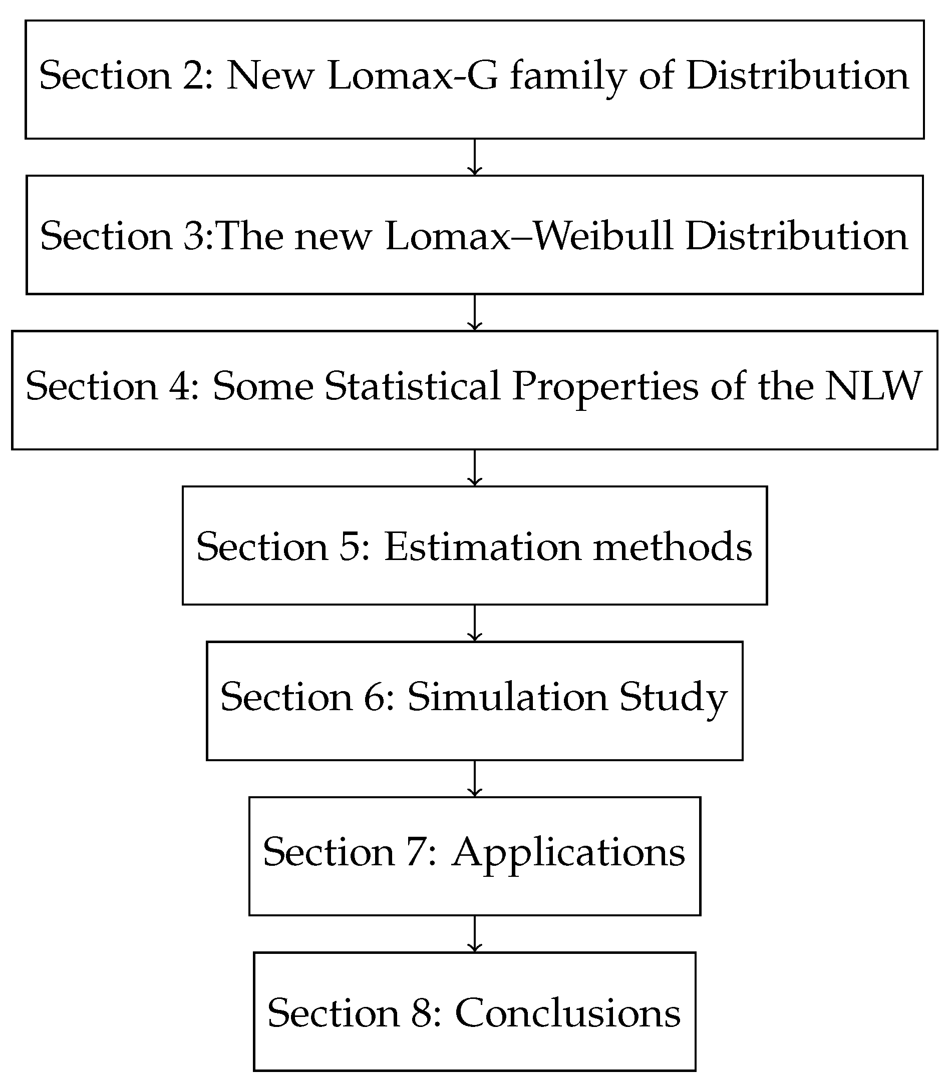
2. New Lomax-G Family of Distribution
3. The New Lomax–Weibull Distribution
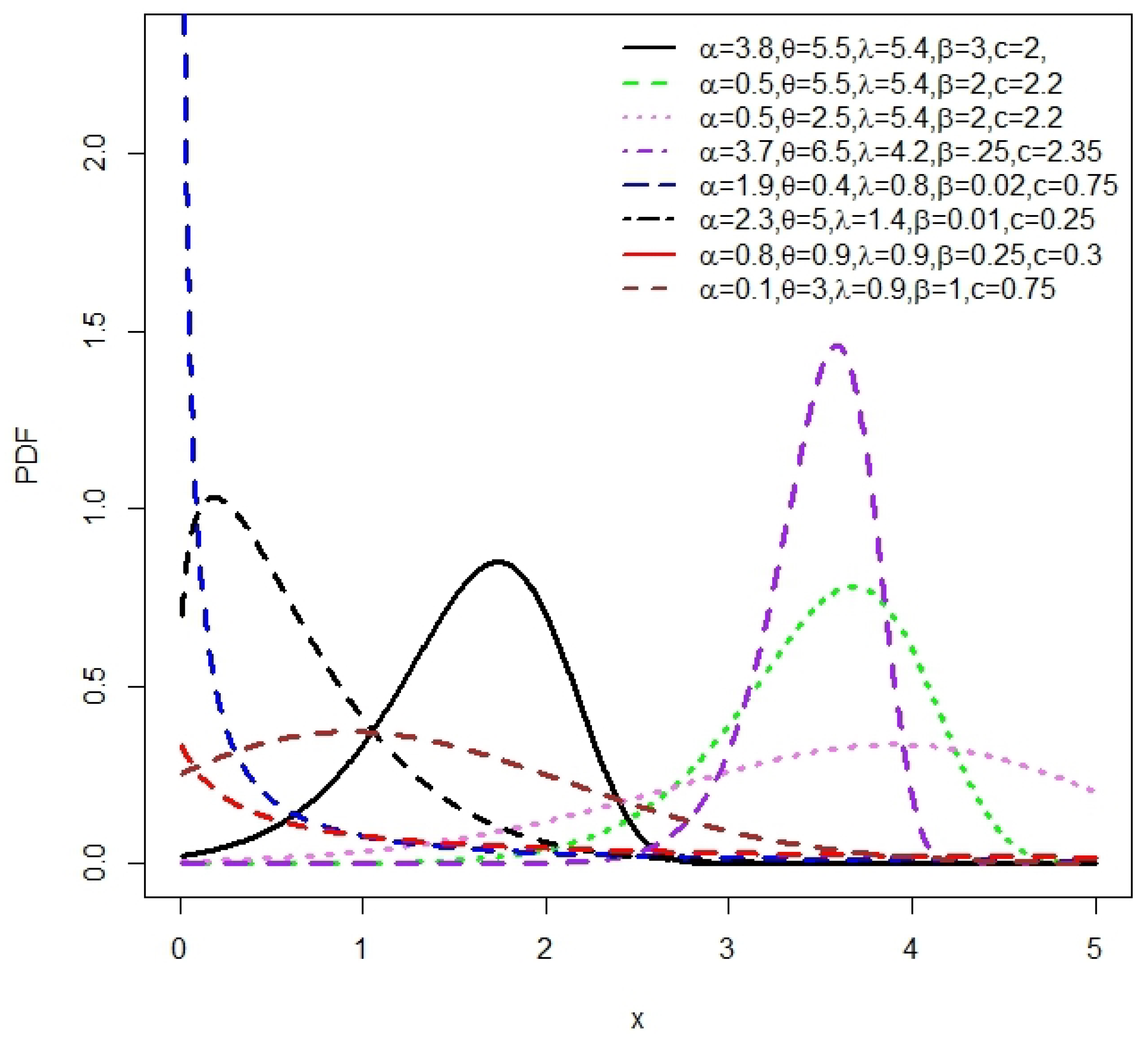
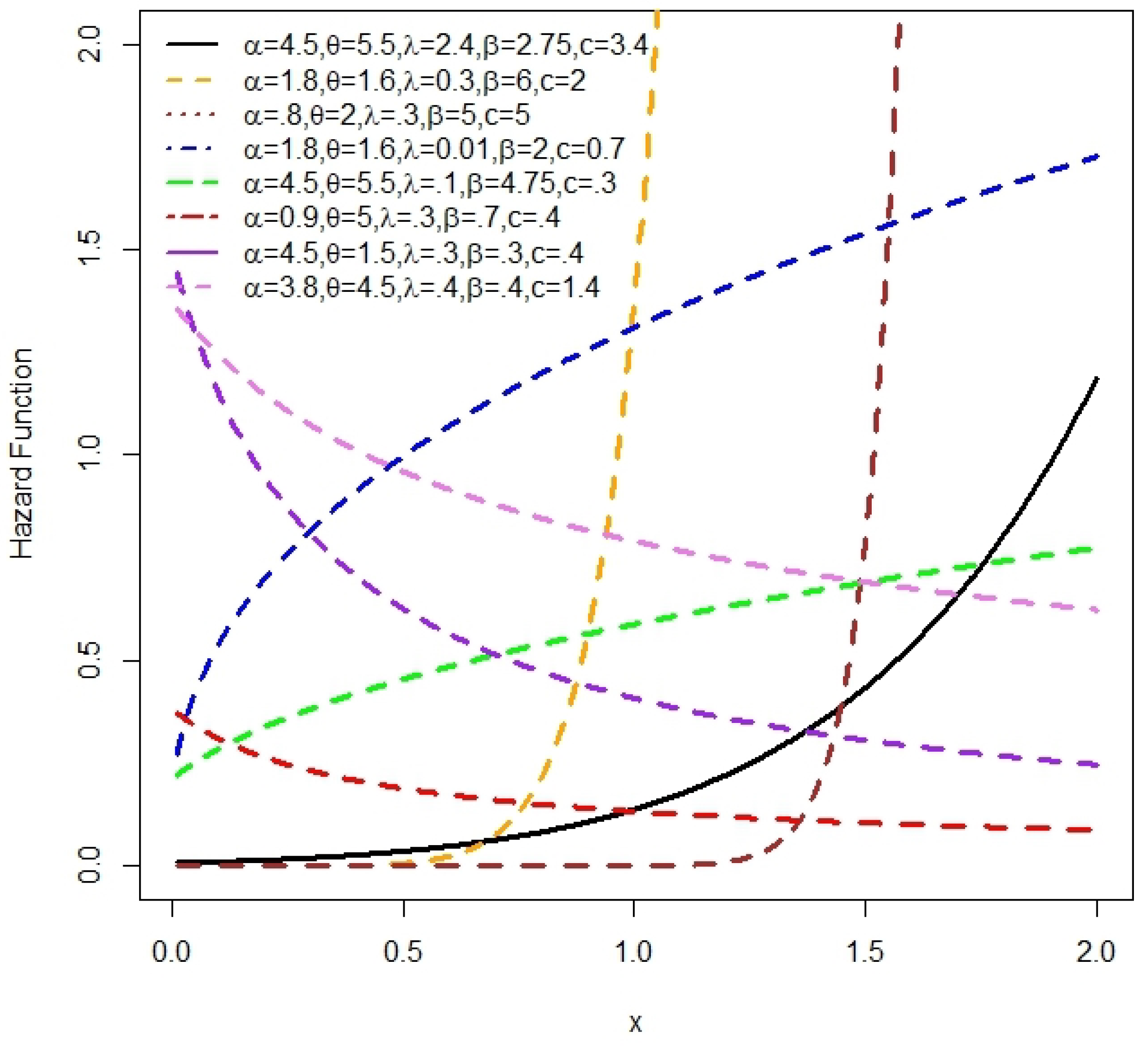
3.1. Graphical Presentations of the NLW
3.2. Special Cases of the NLW Distribution
3.3. Useful Form of the NLW Density
4. Some Statistical Properties of the NLW
4.1. Quantile Function
4.2. Moments
4.3. Moment Generating Function
4.4. Characteristic Function
4.5. Probability Weighted Moment
4.6. Order Statistics
4.7. R’enyi Entropy
4.8. Shannon Entropy
5. Estimation Methods
5.1. Maximum Likelihood Method
5.2. Percentiles Method
5.3. Ordinary and Weighted Least Squares Estimators
5.4. Ke Cramer–von Mises Minimum Distance Method
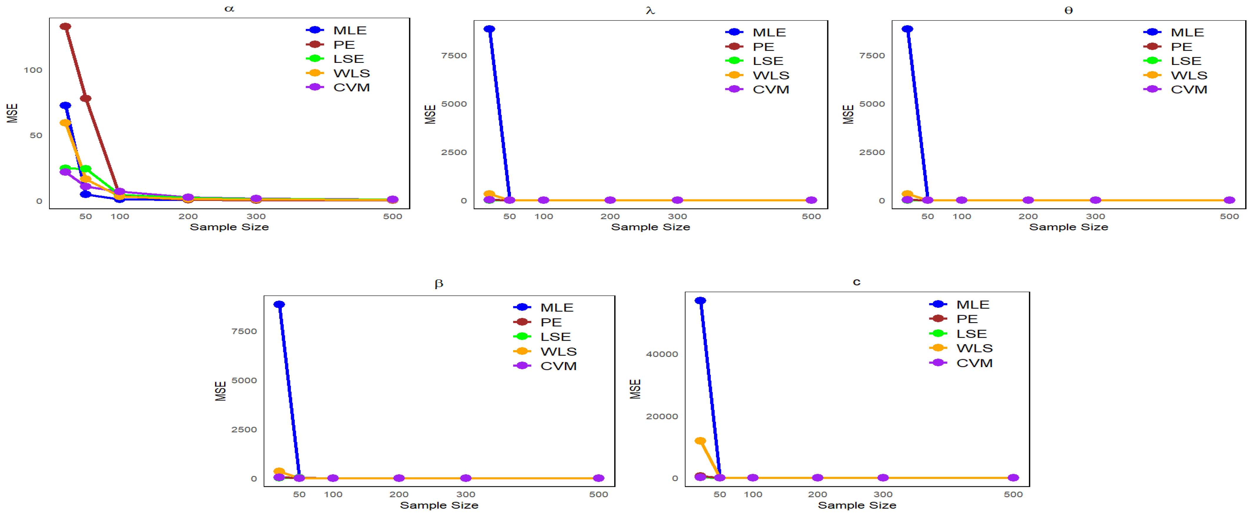
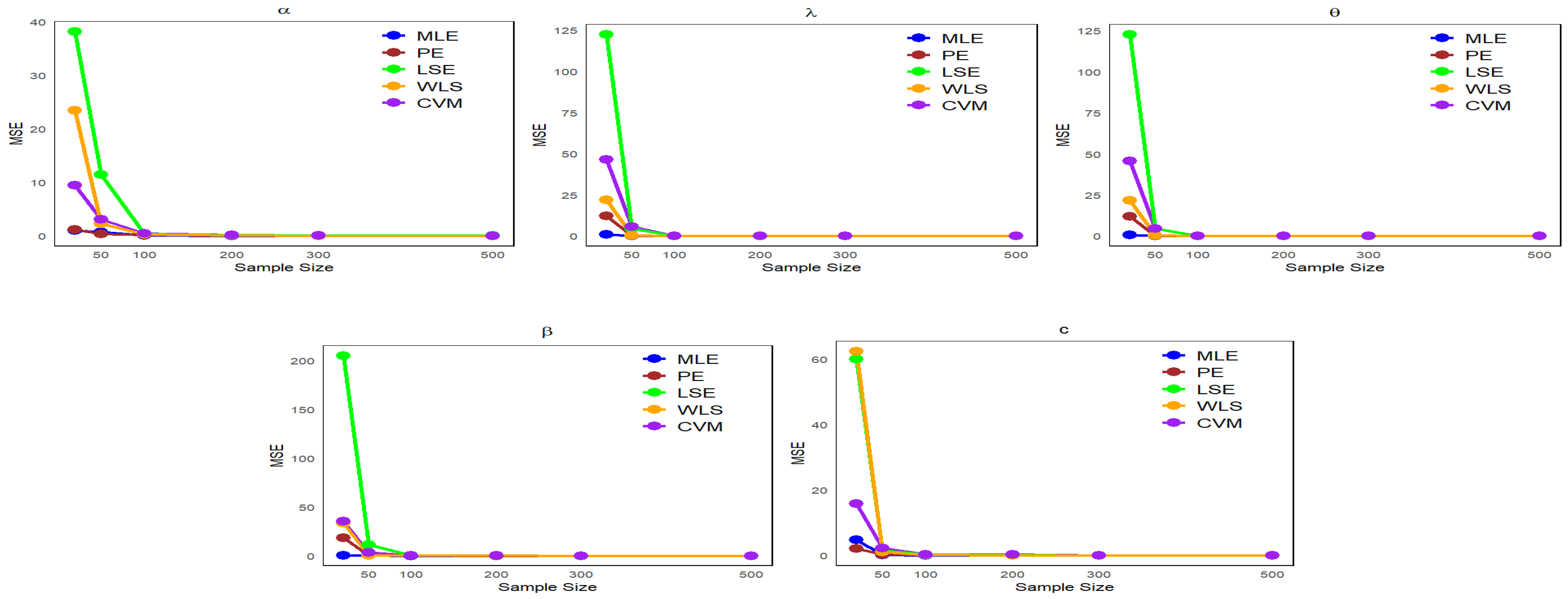
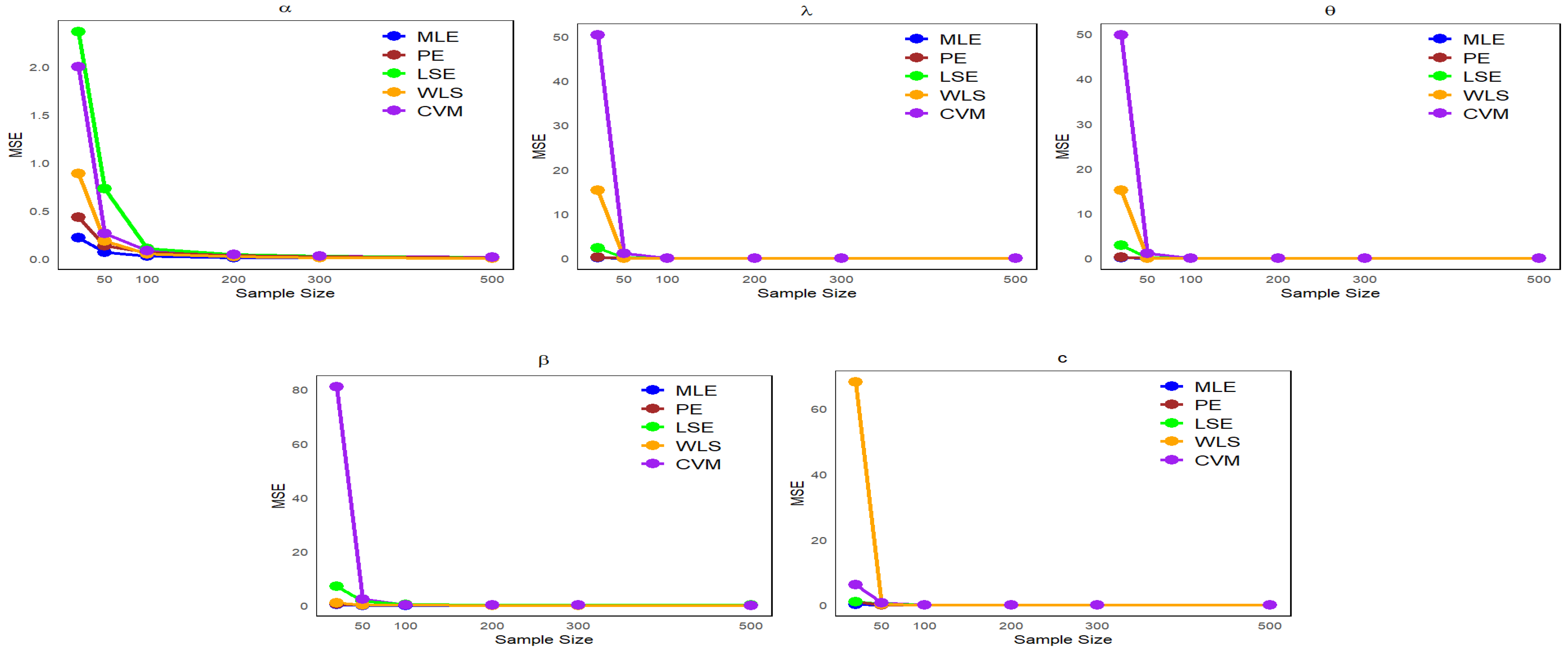
6. Simulation Study
- Data are generated from the NLW distribution as described in Equation (17), with .
- We examine multiple sample sizes (20, 50, 100, 200, 300, and 500) from the NLW, each under 1000 repetitions.
- Four distinct sets of parameter values are defined as follows:
- -
- Set I: (
- -
- Set II:
- -
- Set III:
- -
- Set IV:
7. Applications
- Failure Time Data:
- The first dataset, obtained from [17], represents 84 recorded failure times of aircraft windshields, described as follows: 0.040, 1.866, 2.385, 3.443, 0.301, 1.876, 2.481, 3.467, 0.309, 1.899, 2.610, 3.478, 0.557, 1.911, 2.625, 3.578, 0.943, 1.912, 2.632, 3.595, 1.070, 1.914, 2.646, 3.699, 1.124, 1.981, 2.661, 3.779, 1.248, 2.010, 2.688, 3.924, 1.281, 2.038, 2.823, 4.035, 1.281, 2.085, 2.890, 4.121, 1.303, 2.089, 2.902, 4.167, 1.432, 2.097, 2.934, 4.240, 1.480, 2.135, 2.962, 4.255, 1.505, 2.154, 2.964, 4.278, 1.506, 2.190, 3.000, 4.305, 1.568, 2.194, 3.103, 4.376, 1.615, 2.223, 3.114, 4.449, 1.619, 2.224, 3.117, 4.485, 1.652, 2.229, 3.166, 4.570, 1.652, 2.300, 3.344, 4.602, 1.757, 2.324, 3.376, 4.663.
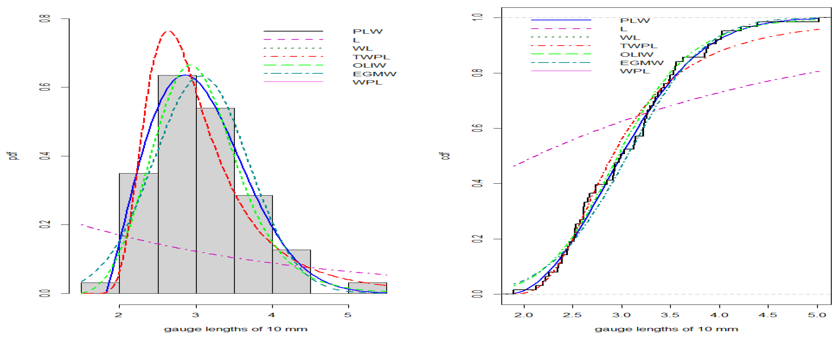
- Gauge Lengths of 10 mm Data:
- The second dataset was obtained from [18] and consists of 63 observations: 1.901, 2.132, 2.203, 2.228, 2.257, 2.350, 2.361, 2.396, 2.397, 2.445, 2.454, 2.474, 2.518, 2.522, 2.525, 2.532, 2.575, 2.614, 2.616, 2.618, 2.624, 2.659, 2.675, 2.738, 2.740, 2.856, 2.917, 2.928, 2.937, 2.937, 2.977, 2.996, 3.030, 3.125, 3.139, 3.145, 3.220, 3.223, 3.235, 3.243, 3.264, 3.272, 3.294, 3.332, 3.346, 3.377, 3.408, 3.435, 3.493, 3.501, 3.537, 3.554, 3.562, 3.628, 3.852, 3.871, 3.886, 3.971, 4.024, 4.027, 4.225, 4.395, 5.020.
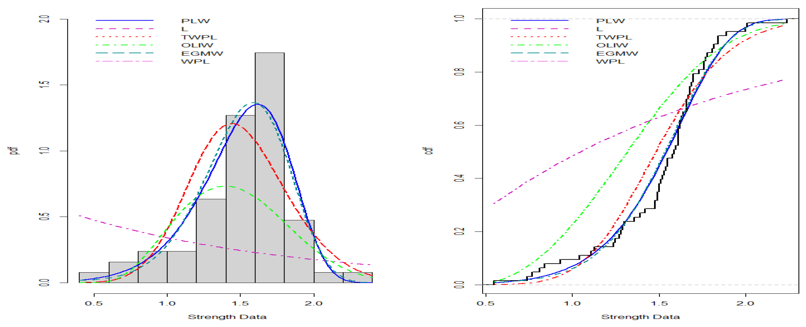
- Strength Data:
- The third dataset, sourced from [19], includes 63 observations: 0.55, 0.74, 0.77, 0.81, 0.84, 1.24, 0.93, 1.04, 1.11, 1.13, 1.30, 1.25, 1.27, 1.28, 1.29, 1.48, 1.36, 1.39, 1.42, 1.48, 1.51, 1.49, 1.49, 1.50, 1.50, 1.55, 1.52, 1.53, 1.54, 1.55, 1.61, 1.58, 1.59, 1.60, 1.61, 1.63, 1.61, 1.61, 1.62, 1.62, 1.67, 1.64, 1.66, 1.66, 1.66, 1.70, 1.68, 1.68, 1.69, 1.70, 1.78, 1.73, 1.76, 1.76, 1.77, 1.89, 1.81, 1.82, 1.84, 1.84, 2.00, 2.01, 2.24.
- Student Grades in Mathematics Data:
- The fourth dataset represents the mathematical scores of 48 students in the slow pace program in the year 2013, sourced from [20]. The data are as follows: 29, 25, 50, 15, 13, 27, 15, 18, 7, 7, 8, 19, 12, 18, 5, 21, 15, 86, 21, 15, 14, 39, 15, 14, 70, 44, 6, 23, 58, 19, 50, 23, 11, 6, 34, 18, 28, 34, 12, 37, 4, 60, 20, 23, 40, 65, 19, and 31.
8. Conclusions
Author Contributions
Funding
Data Availability Statement
Conflicts of Interest
References
- Alzaatreh, A.; Lee, C.; Famoye, F. A new method for generating families of continuous distributions. Metron 2013, 71, 63–79. [Google Scholar] [CrossRef]
- Alzaatreh, A.; Famoye, F.; Lee, C. Weibull–Pareto distribution and its applications. Commun. Stat. Theory Methods 2013, 42, 1673–1691. [Google Scholar] [CrossRef]
- Alzaghal, A.; Famoye, F.; Lee, C. Exponentiated TX family of distributions with some applications. Int. J. Stat. Probab. 2013, 2, 31. [Google Scholar] [CrossRef]
- Famoye, F.; Akarawak, E.; Ekum, M. Weibull–Normal distribution and its applications. J. Stat. Theory Appl. 2018, 17, 719–727. [Google Scholar] [CrossRef]
- Cordeiro, G.M.; Alizadeh, M.; Ozel, G.; Hosseini, B.; Ortega, E.M.M.; Altun, E. The generalized odd log-logistic family of distributions: Properties, regression models and applications. J. Stat. Comput. Simul. 2017, 87, 908–932. [Google Scholar] [CrossRef]
- Reyad, H.; Selim, M.A.; Othman, S. The Nadarajah Haghighi Topp Leone-G Family of distributions with mathematical properties and applications. Pak. J. Stat. Oper. Res. 2019, 15, 849–866. [Google Scholar] [CrossRef]
- Cordeiro, G.; Afify, A.; Ortega, E.; Suzuki, A.; Mead, M. The odd Lomax generator of distributions: Properties, estimation and applications. J. Comput. Appl. Math. 2019, 347, 222–237. [Google Scholar] [CrossRef]
- Aslam, M.; Asghar, Z.; Hussain, Z.; Shah, S.F. A modified TX family of distributions: Classical and Bayesian analysis. J. Taibah Univ. Sci. 2020, 14, 254–264. [Google Scholar] [CrossRef]
- Ahmad, Z.; Mahmoudi, E.; Alizadeh, M.; Roozegar, R.; Afify, A. The exponential TX family of distributions: Properties and an application to insurance data. J. Math. 2021, 2017, 1–18. [Google Scholar]
- Klakattawi, H.; Alsulami, D.; Elaal, M.; Dey, S.; Baharith, L. A new generalized family of distributions based on combining Marshal-Olkin transformation with TX family. PLoS ONE 2022, 17, e0263673. [Google Scholar] [CrossRef] [PubMed]
- Shah, Z.; Khan, D.; Khan, Z.; Faiz, N.; Hussain, S.; Anwar, A.; Ahmad, T.; Kim, K. A New Generalized Logarithmic–X Family of Distributions with Biomedical Data Analysis. Appl. Sci. 2023, 13, 3668. [Google Scholar] [CrossRef]
- Ahmad, M.; Jabeen, R.; Zaka, A.; Hamdi, W.; Alnssyan, B. A unified generalized family of distributions: Properties, inference, and real-life applications. AIP Adv. 2024, 14, 015043. [Google Scholar] [CrossRef]
- Mills, J.P. Table of the ratio: Area to bounding ordinate, for any portion of normal curve. Biometrika 1926, 18, 395–400. [Google Scholar] [CrossRef]
- Nagy, M.; Ahmad, M.; Jabeen, R.; Zaka, A.; Alrasheedi, A.; Mansi, A.H. Evaluation of survival weighted Pareto distribution: Analytical properties and applications to industrial and aeronautics data. AIP Adv. 2024, 14, 045140. [Google Scholar] [CrossRef]
- Jabeen, R.; Ahmad, M.; Zaka, A.; Mansour, M.M.; Aljadani, A.; Abd Elrazik, E.M. A New Statistical Approach Based on the Access of Electricity Application with Some Modified Control Charts. J. Math. 2024, 1, 6584791. [Google Scholar] [CrossRef]
- R Core Team. R: A Language and Environment for Statistical Computing; R Foundation for Statistical Computing: Vienna, Austria, 2023; Available online: https://www.R-project.org/ (accessed on 25 January 2024).
- Tahir, M.H.; Cordeiro, G.M.; Mansoor, M.; Zubair, M. The Weibull-Lomax distribution: Properties and applications. Hacet. J. Math. Stat. 2015, 44, 455–474. [Google Scholar] [CrossRef]
- Kundu, D.; Raqab, M.Z. Estimation of R = P (Y< X) for three-parameter Weibull distribution. Stat. Probab. Lett. 2009, 79, 1839–1846. [Google Scholar]
- Smith, R.L.; Naylor, J. A comparison of maximum likelihood and Bayesian estimators for the three-parameter Weibull distribution. J. R. Stat. Soc. Ser. Appl. Stat. 1987, 36, 358–369. [Google Scholar] [CrossRef]
- ZeinEldin, R.A.; Ahsan ul Haq, M.; Hashmi, S.; Elsehety, M. Alpha power transformed inverse Lomax distribution with different methods of estimation and applications. Complexity 2020, 2020, 1860813. [Google Scholar] [CrossRef]
- Al-Marzouki, S. Truncated Weibull power Lomax distribution: Statistical properties and applications. J. Nonlinear Sci. Appl. 2019, 12, 543–551. [Google Scholar] [CrossRef]
- Almetwally, E.M. Application of COVID-19 pandemic by using odd lomax-G inverse Weibull distribution. Math. Sci. Lett. 2021, 10, 47–57. [Google Scholar]
- Aryal, G.; Elbatal, I. On the exponentiated generalized modified Weibull distribution. Commun. Stat. Appl. Methods 2015, 22, 333–348. [Google Scholar] [CrossRef]


| Set I: | MLE | PE | LSE | WLS | CVM | |||||||||||
|---|---|---|---|---|---|---|---|---|---|---|---|---|---|---|---|---|
| Est | Bias | MSE | Est | Bias | MSE | Est | Bias | MSE | Est | Bias | MSE | Est | Bias | MSE | ||
| 2.8325 | 1.1825 | 72.398 | 2.6589 | 1.0089 | 132.64 | 2.3626 | 0.7126 | 24.436 | 2.6864 | 1.0364 | 59.301 | 2.5847 | 0.9347 | 21.647 | ||
| 5.1111 | 5.0561 | 8850.1 | 1.0389 | 0.9839 | 39.867 | 0.7355 | 0.6805 | 12.033 | 1.2694 | 1.2144 | 336.58 | 0.7673 | 0.7123 | 32.162 | ||
| n = 20 | 5.6321 | 5.0421 | 8849.2 | 1.5375 | 0.9475 | 39.972 | 1.2582 | 0.6682 | 12.088 | 1.7878 | 1.1978 | 336.61 | 1.2956 | 0.7056 | 32.190 | |
| 8.4348 | 6.4548 | 17,322 | 4.7218 | 2.7418 | 404.88 | 3.8820 | 1.9020 | 156.54 | 3.8012 | 1.8212 | 88.329 | 4.7230 | 2.7430 | 558.78 | ||
| c | 17.342 | 14.842 | 57,031 | 4.9615 | 2.4615 | 528.04 | 4.4392 | 1.9392 | 163.37 | 8.2053 | 5.7053 | 11,922 | 4.2164 | 1.7164 | 115.83 | |
| 1.9553 | 0.3053 | 4.5297 | 2.4883 | 0.8383 | 77.746 | 2.3747 | 0.7247 | 24.084 | 2.1694 | 0.5194 | 16.214 | 2.2274 | 0.5774 | 10.746 | ||
| 0.2441 | 0.1891 | 1.3782 | 0.5950 | 0.5400 | 13.540 | 0.4685 | 0.4135 | 4.4953 | 0.3447 | 0.2897 | 1.9793 | 0.3371 | 0.2821 | 1.9451 | ||
| n = 50 | 0.7697 | 0.1797 | 1.3349 | 1.1145 | 0.5245 | 13.632 | 1.0008 | 0.4108 | 4.5406 | 0.8682 | 0.2782 | 2.0244 | 0.8665 | 0.2765 | 1.9879 | |
| 2.6559 | 0.6759 | 20.546 | 3.9032 | 1.9232 | 185.936 | 3.2885 | 1.3085 | 55.768 | 2.8668 | 0.8868 | 43.128 | 3.0731 | 1.0931 | 32.324 | ||
| c | 3.1397 | 0.6397 | 33.975 | 3.5148 | 1.0148 | 46.820 | 3.7666 | 1.2666 | 61.384 | 3.5547 | 1.0547 | 35.8343 | 3.5488 | 1.0488 | 36.623 | |
| 1.7792 | 0.1292 | 0.9413 | 1.8632 | 0.2132 | 3.2869 | 2.0475 | 0.3975 | 4.3204 | 1.9690 | 0.3190 | 3.1240 | 2.2048 | 0.5548 | 6.9803 | ||
| 0.0942 | 0.0392 | 0.0736 | 0.2019 | 0.1469 | 1.4697 | 0.2056 | 0.1506 | 0.3953 | 0.1863 | 0.1313 | 0.4331 | 0.2465 | 0.1915 | 1.4830 | ||
| n = 100 | 0.6237 | 0.0337 | 0.0591 | 0.7299 | 0.1399 | 1.4916 | 0.7389 | 0.1489 | 0.4042 | 0.7174 | 0.1274 | 0.4330 | 0.7825 | 0.1925 | 1.5185 | |
| 2.2200 | 0.2400 | 2.5263 | 2.4232 | 0.4432 | 15.3716 | 2.5633 | 0.5833 | 10.510 | 2.3945 | 0.4145 | 4.0481 | 2.5336 | 0.5536 | 8.0548 | ||
| c | 2.6651 | 0.1651 | 1.2119 | 2.8840 | 0.3840 | 10.539 | 3.1386 | 0.6386 | 11.385 | 3.0895 | 0.5895 | 11.886 | 3.6041 | 1.1041 | 28.298 | |
| 1.7746 | 0.1246 | 0.3944 | 1.6937 | 0.0437 | 0.5465 | 1.8919 | 0.2419 | 2.1012 | 1.7869 | 0.1369 | 1.1100 | 1.9395 | 0.2895 | 2.4003 | ||
| 0.0671 | 0.0121 | 0.0154 | 0.1021 | 0.0471 | 0.0224 | 0.1483 | 0.0933 | 0.1531 | 0.1062 | 0.0512 | 0.0786 | 0.1371 | 0.0821 | 0.1316 | ||
| n = 200 | 0.6044 | 0.0144 | 0.0124 | 0.6317 | 0.0417 | 0.0192 | 0.6827 | 0.0927 | 0.1577 | 0.6372 | 0.0472 | 0.0808 | 0.6720 | 0.0820 | 0.1378 | |
| 2.0513 | 0.0713 | 0.3637 | 2.0980 | 0.1180 | 0.8957 | 2.2493 | 0.2693 | 2.8724 | 2.1583 | 0.1783 | 1.2778 | 2.2319 | 0.2519 | 1.8202 | ||
| c | 2.5894 | 0.0894 | 0.5197 | 2.7698 | 0.2698 | 1.1236 | 3.0235 | 0.5235 | 5.7526 | 2.8152 | 0.3152 | 3.4335 | 3.1113 | 0.6113 | 9.9644 | |
| 1.7939 | 0.1439 | 0.2853 | 1.6876 | 0.0376 | 0.3301 | 1.8286 | 0.1786 | 1.2810 | 1.7377 | 0.0877 | 0.7493 | 1.8746 | 0.2246 | 1.5704 | ||
| 0.0585 | 0.0035 | 0.0084 | 0.0830 | 0.0280 | 0.0114 | 0.0996 | 0.0446 | 0.0371 | 0.0850 | 0.0300 | 0.0185 | 0.1161 | 0.0611 | 0.0741 | ||
| n = 300 | 0.5997 | 0.0097 | 0.0073 | 0.6152 | 0.0252 | 0.0102 | 0.6331 | 0.0431 | 0.0385 | 0.6163 | 0.0263 | 0.0182 | 0.6508 | 0.0608 | 0.0797 | |
| 2.0125 | 0.0325 | 0.2397 | 2.0160 | 0.0360 | 0.3186 | 2.1325 | 0.1525 | 0.9961 | 2.1486 | 0.1686 | 0.7590 | 2.2211 | 0.2411 | 1.4580 | ||
| c | 2.5625 | 0.0625 | 0.3312 | 2.7001 | 0.2001 | 0.7051 | 2.8599 | 0.3599 | 2.5825 | 2.6639 | 0.1639 | 1.0250 | 2.8540 | 0.3540 | 3.5211 | |
| 1.7493 | 0.0993 | 0.1477 | 1.6977 | 0.0477 | 0.2407 | 1.8173 | 0.1673 | 0.9646 | 1.7547 | 0.1047 | 0.3717 | 1.8012 | 0.1512 | 0.7829 | ||
| 0.0549 | 0.0001 | 0.0043 | 0.0729 | 0.0179 | 0.0058 | 0.0848 | 0.0298 | 0.0200 | 0.0748 | 0.0198 | 0.0095 | 0.0906 | 0.0356 | 0.0219 | ||
| n = 500 | 0.5947 | 0.0047 | 0.0042 | 0.6081 | 0.0181 | 0.0063 | 0.6214 | 0.0314 | 0.0223 | 0.6113 | 0.0213 | 0.0111 | 0.6259 | 0.0359 | 0.0256 | |
| 1.9680 | 0.0120 | 0.1007 | 1.9842 | 0.0042 | 0.1723 | 2.0938 | 0.1138 | 0.8366 | 2.0574 | 0.0774 | 0.3413 | 2.0809 | 0.1009 | 0.5584 | ||
| c | 2.5651 | 0.0651 | 0.1959 | 2.6496 | 0.1496 | 0.3651 | 2.7682 | 0.2682 | 1.4894 | 2.6361 | 0.1361 | 0.6002 | 2.7961 | 0.2961 | 1.5130 |
| Set II: | MLE | PE | LSE | WLS | CVM | |||||||||||
|---|---|---|---|---|---|---|---|---|---|---|---|---|---|---|---|---|
| Est | Bias | MSE | Est | Bias | MSE | Est | Bias | MSE | Est | Bias | MSE | Est | Bias | MSE | ||
| 2.1252 | 0.2252 | 1.0045 | 1.7955 | 0.1045 | 1.2215 | 2.2165 | 0.3165 | 38.1752 | 2.0635 | 0.1635 | 23.4578 | 1.9887 | 0.0887 | 9.5050 | ||
| 0.0987 | 0.0287 | 1.1627 | 0.5046 | 0.4346 | 12.358 | 1.6284 | 1.5584 | 122.41 | 0.9587 | 0.8887 | 21.980 | 1.1731 | 1.1031 | 46.391 | ||
| n = 20 | 2.5924 | 0.0924 | 0.7104 | 2.8532 | 0.3532 | 11.936 | 3.8656 | 1.3656 | 122.62 | 3.2268 | 0.7268 | 21.743 | 3.3836 | 0.8836 | 45.636 | |
| 1.2414 | 0.0414 | 0.4173 | 1.5393 | 0.3393 | 18.189 | 2.8180 | 1.6180 | 204.99 | 2.0297 | 0.8297 | 33.370 | 2.0745 | 0.8745 | 35.206 | ||
| c | 2.1433 | 0.2433 | 4.7736 | 2.1248 | 0.2248 | 2.0812 | 2.6289 | 0.7289 | 59.894 | 2.6107 | 0.7107 | 62.280 | 2.5608 | 0.6608 | 15.909 | |
| 2.1307 | 0.2307 | 0.7892 | 1.9076 | 0.0076 | 0.3990 | 1.9119 | 0.0119 | 11.4561 | 1.8608 | 0.0392 | 2.2713 | 1.9803 | 0.0803 | 3.1521 | ||
| 0.0065 | 0.0635 | 0.0832 | 0.1508 | 0.0808 | 0.1940 | 0.4593 | 0.3893 | 4.4835 | 0.2731 | 0.2031 | 0.5199 | 0.3960 | 0.3260 | 5.5061 | ||
| n = 50 | 2.5415 | 0.0415 | 0.0649 | 2.6125 | 0.1125 | 0.1047 | 2.7698 | 0.2698 | 4.4822 | 2.6272 | 0.1272 | 0.4337 | 2.7516 | 0.2516 | 5.4158 | |
| 1.2106 | 0.0106 | 0.1642 | 1.2528 | 0.0528 | 0.2828 | 1.5703 | 0.3703 | 11.2381 | 1.3601 | 0.1601 | 0.4883 | 1.4959 | 0.2959 | 3.5417 | ||
| c | 1.9035 | 0.0035 | 0.2328 | 1.9896 | 0.0896 | 0.3995 | 2.1333 | 0.2333 | 1.5769 | 2.0581 | 0.1581 | 1.0788 | 2.1096 | 0.2096 | 2.3547 | |
| 2.0788 | 0.1788 | 0.1316 | 1.9657 | 0.0657 | 0.1995 | 1.8549 | 0.0451 | 0.4114 | 1.9071 | 0.0071 | 0.3292 | 1.9115 | 0.0115 | 0.4935 | ||
| 0.0211 | 0.0489 | 0.0265 | 0.0808 | 0.0108 | 0.0738 | 0.2438 | 0.1738 | 0.2795 | 0.1624 | 0.0924 | 0.0945 | 0.1821 | 0.1121 | 0.1618 | ||
| n = 100 | 2.5468 | 0.0468 | 0.0200 | 2.5660 | 0.0660 | 0.0444 | 2.6163 | 0.1163 | 0.2021 | 2.5788 | 0.0788 | 0.0859 | 2.5791 | 0.0791 | 0.1117 | |
| 1.1956 | 0.0044 | 0.0479 | 1.1971 | 0.0029 | 0.0970 | 1.3539 | 0.1539 | 0.4883 | 1.2887 | 0.0887 | 0.1772 | 1.3357 | 0.1357 | 0.4655 | ||
| c | 1.8834 | 0.0166 | 0.0563 | 1.9369 | 0.0369 | 0.1656 | 2.0044 | 0.1044 | 0.3875 | 1.9593 | 0.0593 | 0.2628 | 1.9822 | 0.0822 | 0.3541 | |
| 2.0424 | 0.1424 | 0.0618 | 1.9764 | 0.0764 | 0.0981 | 1.9197 | 0.0197 | 0.1855 | 1.9314 | 0.0314 | 0.1041 | 1.9408 | 0.0408 | 0.2055 | ||
| 0.0362 | 0.0338 | 0.0118 | 0.0713 | 0.0013 | 0.0285 | 0.1559 | 0.0859 | 0.0747 | 0.1151 | 0.0451 | 0.0304 | 0.1499 | 0.0799 | 0.0726 | ||
| n = 200 | 2.5430 | 0.0430 | 0.0106 | 2.5541 | 0.0541 | 0.0229 | 2.5829 | 0.0829 | 0.0807 | 2.5576 | 0.0576 | 0.0320 | 2.5777 | 0.0777 | 0.0798 | |
| 1.1797 | 0.0203 | 0.0150 | 1.1957 | 0.0043 | 0.0393 | 1.2819 | 0.0819 | 0.1564 | 1.2524 | 0.0524 | 0.0969 | 1.2743 | 0.0743 | 0.1435 | ||
| c | 1.9053 | 0.0053 | 0.0298 | 1.9218 | 0.0218 | 0.0787 | 1.9495 | 0.0495 | 0.2030 | 1.9231 | 0.0231 | 0.0920 | 1.9752 | 0.0752 | 0.2719 | |
| 2.0166 | 0.1166 | 0.0380 | 1.9730 | 0.0730 | 0.0558 | 1.9596 | 0.0596 | 0.1138 | 1.9487 | 0.0487 | 0.0529 | 1.9567 | 0.0567 | 0.1642 | ||
| 0.0434 | 0.0266 | 0.0069 | 0.0610 | 0.0090 | 0.0168 | 0.1309 | 0.0609 | 0.0433 | 0.1002 | 0.0302 | 0.0177 | 0.1272 | 0.0572 | 0.0400 | ||
| n = 300 | 2.5379 | 0.0379 | 0.0078 | 2.5436 | 0.0436 | 0.0156 | 2.5871 | 0.0871 | 0.0524 | 2.5544 | 0.0544 | 0.0205 | 2.5721 | 0.0721 | 0.0601 | |
| 1.1803 | 0.0197 | 0.0089 | 1.1883 | 0.0117 | 0.0261 | 1.2590 | 0.0590 | 0.0888 | 1.2213 | 0.0213 | 0.0329 | 1.2619 | 0.0619 | 0.0853 | ||
| c | 1.9060 | 0.0060 | 0.0150 | 1.9117 | 0.0117 | 0.0440 | 1.9288 | 0.0288 | 0.1138 | 1.9270 | 0.0270 | 0.0504 | 1.9278 | 0.0278 | 0.1087 | |
| 2.0036 | 0.1036 | 0.0245 | 1.9669 | 0.0669 | 0.0336 | 1.9546 | 0.0546 | 0.0943 | 1.9447 | 0.0447 | 0.0283 | 1.9516 | 0.0516 | 0.0640 | ||
| 0.0491 | 0.0209 | 0.0039 | 0.0630 | 0.0070 | 0.0104 | 0.1132 | 0.0432 | 0.0238 | 0.0909 | 0.0209 | 0.0099 | 0.1044 | 0.0344 | 0.0207 | ||
| n = 500 | 2.5361 | 0.0361 | 0.0048 | 2.5364 | 0.0364 | 0.0123 | 2.5675 | 0.0675 | 0.0411 | 2.5441 | 0.0441 | 0.0117 | 2.5555 | 0.0555 | 0.0283 | |
| 1.1843 | 0.0157 | 0.0048 | 1.1931 | 0.0069 | 0.0188 | 1.2515 | 0.0515 | 0.0757 | 1.2181 | 0.0181 | 0.0181 | 1.2381 | 0.0381 | 0.0451 | ||
| c | 1.9033 | 0.0033 | 0.0068 | 1.9022 | 0.0022 | 0.0249 | 1.9078 | 0.0078 | 0.0626 | 1.9130 | 0.0130 | 0.0310 | 1.9124 | 0.0124 | 0.0653 |
| Set III: | MLE | PE | LSE | WLS | CVM | |||||||||||
|---|---|---|---|---|---|---|---|---|---|---|---|---|---|---|---|---|
| Est | Bias | MSE | Est | Bias | MSE | Est | Bias | MSE | Est | Bias | MSE | Est | Bias | MSE | ||
| 1.5814 | 0.1814 | 0.2225 | 1.3867 | 0.0133 | 0.4314 | 1.3496 | 0.0504 | 2.9444 | 1.2654 | 0.1346 | 0.8901 | 1.3059 | 0.0941 | 2.0009 | ||
| 0.0746 | 0.0424 | 0.1545 | 0.2214 | 0.1044 | 0.3504 | 0.4121 | 0.2951 | 2.4036 | 0.5367 | 0.4197 | 15.3767 | 0.6711 | 0.5541 | 50.310 | ||
| n = 20 | 1.2910 | 0.0210 | 0.1152 | 1.3797 | 0.1097 | 0.2618 | 1.4575 | 0.1875 | 2.3614 | 1.5732 | 0.3032 | 15.1566 | 1.6915 | 0.4215 | 49.765 | |
| 1.1544 | 0.0456 | 0.2761 | 1.2256 | 0.0256 | 0.5083 | 1.5165 | 0.3165 | 7.0105 | 1.4214 | 0.2214 | 0.9747 | 1.9180 | 0.7180 | 81.094 | ||
| c | 1.4935 | 0.0435 | 0.1782 | 1.6275 | 0.1775 | 0.9548 | 1.6856 | 0.2356 | 0.9860 | 2.1021 | 0.6521 | 68.0949 | 1.8635 | 0.4135 | 6.3057 | |
| 1.5401 | 0.1401 | 0.0695 | 1.4383 | 0.0383 | 0.1391 | 1.3837 | 0.0163 | 0.7334 | 1.3676 | 0.0324 | 0.1852 | 1.3744 | 0.0256 | 0.2641 | ||
| 0.0303 | 0.0420 | 0.0089 | 0.1317 | 0.0147 | 0.0402 | 0.2378 | 0.1028 | 0.2232 | 0.1774 | 0.0604 | 0.0359 | 0.2257 | 0.1087 | 1.1197 | ||
| n = 50 | 1.2853 | 0.0153 | 0.0086 | 1.3213 | 0.0513 | 0.0279 | 1.3599 | 0.0899 | 0.2176 | 1.3127 | 0.0427 | 0.0309 | 1.3420 | 0.0720 | 1.0761 | |
| 1.1601 | 0.0399 | 0.0366 | 1.1825 | 0.0175 | 0.1378 | 1.3661 | 0.1661 | 1.5103 | 1.2650 | 0.0650 | 0.1321 | 1.3136 | 0.1136 | 0.2900 | ||
| c | 1.4544 | 0.0044 | 0.0275 | 1.5086 | 0.0586 | 0.0880 | 1.5638 | 0.1138 | 0.3710 | 1.5307 | 0.0807 | 0.2350 | 1.6342 | 0.1842 | 7.0338 | |
| 1.5092 | 0.1092 | 0.0299 | 1.4693 | 0.0693 | 0.0684 | 1.3735 | 0.0265 | 0.1108 | 1.4093 | 0.0093 | 0.0539 | 1.3948 | 0.0052 | 0.0878 | ||
| 0.0151 | 0.0268 | 0.0032 | 0.1065 | 0.0105 | 0.0141 | 0.1755 | 0.0855 | 0.0291 | 0.1453 | 0.0283 | 0.0093 | 0.1565 | 0.0395 | 0.0192 | ||
| n = 100 | 1.2901 | 0.0201 | 0.0043 | 1.3020 | 0.0320 | 0.0084 | 1.3114 | 0.0414 | 0.0305 | 1.3024 | 0.0324 | 0.0122 | 1.2991 | 0.0291 | 0.0192 | |
| 1.1656 | 0.0344 | 0.0158 | 1.1521 | 0.0479 | 0.0610 | 1.2856 | 0.0856 | 0.2473 | 1.2326 | 0.0326 | 0.0602 | 1.2536 | 0.0536 | 0.1118 | ||
| c | 1.4579 | 0.0079 | 0.0121 | 1.4930 | 0.0430 | 0.0544 | 1.5013 | 0.0513 | 0.0943 | 1.4849 | 0.0349 | 0.0469 | 1.5166 | 0.0666 | 0.0901 | |
| 1.4828 | 0.0828 | 0.0152 | 1.4629 | 0.0629 | 0.0369 | 1.4020 | 0.0202 | 0.0484 | 1.4203 | 0.0203 | 0.0263 | 1.4056 | 0.0056 | 0.0481 | ||
| 0.0049 | 0.0166 | 0.0012 | 0.1093 | 0.0077 | 0.0063 | 0.1485 | 0.0315 | 0.0082 | 0.1315 | 0.0145 | 0.0029 | 0.1449 | 0.0279 | 0.0074 | ||
| n = 200 | 1.2904 | 0.0204 | 0.0022 | 1.2983 | 0.0283 | 0.0048 | 1.2999 | 0.0299 | 0.0119 | 1.2938 | 0.0238 | 0.0062 | 1.2953 | 0.0253 | 0.0111 | |
| 1.1731 | 0.0269 | 0.0063 | 1.1713 | 0.0287 | 0.0285 | 1.2461 | 0.0461 | 0.0769 | 1.2153 | 0.0153 | 0.0291 | 1.2452 | 0.0452 | 0.0832 | ||
| c | 1.4568 | 0.0068 | 0.0059 | 1.4752 | 0.0252 | 0.0271 | 1.4863 | 0.0363 | 0.0681 | 1.4765 | 0.0265 | 0.0304 | 1.4926 | 0.0426 | 0.0626 | |
| 1.4726 | 0.0726 | 0.0116 | 1.4639 | 0.0639 | 0.0237 | 1.4155 | 0.0155 | 0.0300 | 1.4288 | 0.0288 | 0.0137 | 1.4169 | 0.0169 | 0.0296 | ||
| 0.0006 | 0.0123 | 0.0007 | 0.1072 | 0.0098 | 0.0039 | 0.1401 | 0.0231 | 0.0046 | 0.1272 | 0.0102 | 0.0017 | 0.1385 | 0.0215 | 0.0043 | ||
| n = 300 | 1.2909 | 0.0209 | 0.0016 | 1.2976 | 0.0276 | 0.0033 | 1.2996 | 0.0296 | 0.0090 | 1.2944 | 0.0244 | 0.0035 | 1.2958 | 0.0258 | 0.0083 | |
| 1.1768 | 0.0232 | 0.0036 | 1.1674 | 0.0326 | 0.0184 | 1.2186 | 0.0186 | 0.0571 | 1.2020 | 0.0020 | 0.0189 | 1.2393 | 0.0393 | 0.0544 | ||
| c | 1.4575 | 0.0075 | 0.0032 | 1.4709 | 0.0209 | 0.0195 | 1.4973 | 0.0473 | 0.0553 | 1.4805 | 0.0305 | 0.0239 | 1.4737 | 0.0237 | 0.0378 | |
| 1.4573 | 0.0573 | 0.0066 | 1.4568 | 0.0568 | 0.0149 | 1.4238 | 0.0238 | 0.0131 | 1.4302 | 0.0302 | 0.0066 | 1.4284 | 0.0284 | 0.0168 | ||
| 0.0033 | 0.0084 | 0.0003 | 0.1085 | 0.0085 | 0.0024 | 0.1347 | 0.0177 | 0.0027 | 0.1244 | 0.0074 | 0.0009 | 0.1311 | 0.0141 | 0.0022 | ||
| n = 500 | 1.2886 | 0.0186 | 0.0011 | 1.2919 | 0.0219 | 0.0023 | 1.3000 | 0.0300 | 0.0045 | 1.2930 | 0.0230 | 0.0019 | 1.2960 | 0.0260 | 0.0053 | |
| 1.1811 | 0.0189 | 0.0020 | 1.1822 | 0.0178 | 0.0129 | 1.2216 | 0.0216 | 0.0468 | 1.2009 | 0.0009 | 0.0085 | 1.2157 | 0.0157 | 0.0284 | ||
| c | 1.4578 | 0.0078 | 0.0017 | 1.4548 | 0.0048 | 0.0143 | 1.4777 | 0.0277 | 0.0318 | 1.4709 | 0.0209 | 0.0097 | 1.4729 | 0.0229 | 0.0226 |
| Set IV: | MLE | PE | LSE | WLS | CVM | |||||||||||
|---|---|---|---|---|---|---|---|---|---|---|---|---|---|---|---|---|
| Est | Bias | MSE | Est | Bias | MSE | Est | Bias | MSE | Est | Bias | MSE | Est | Bias | MSE | ||
| 26.959 | 0.5589 | 7.5747 | 28.4682 | 2.0682 | 38.2159 | 27.7222 | 1.3222 | 12.0924 | 27.7749 | 1.3749 | 11.1449 | 27.185 | 0.7850 | 13.618 | ||
| 11.7008 | 0.0008 | 0.0000 | 11.7195 | 0.0195 | 0.3076 | 11.6983 | 0.0017 | 0.0005 | 11.6992 | 0.0008 | 0.0001 | 11.699 | 0.0010 | 0.0015 | ||
| n = 20 | 12.7682 | 0.0018 | 0.0001 | 12.8003 | 0.0303 | 0.3106 | 12.7749 | 0.0049 | 0.0008 | 12.7741 | 0.0041 | 0.0003 | 12.768 | 0.0020 | 0.0028 | |
| 15.7237 | 0.5237 | 6.1200 | 14.6361 | 0.5639 | 7.6170 | 14.7013 | 0.4987 | 8.4308 | 14.9269 | 0.2731 | 6.1488 | 15.6491 | 0.4491 | 10.1611 | ||
| c | 34.5434 | 1.0934 | 9.5238 | 32.9924 | 0.4576 | 11.6788 | 34.3149 | 0.8649 | 10.0987 | 34.0997 | 0.6497 | 12.1072 | 34.8646 | 1.4136 | 14.6085 | |
| 27.5588 | 1.1588 | 4.1070 | 27.8862 | 1.4862 | 23.8686 | 27.6495 | 1.2495 | 7.0637 | 27.502 | 1.1020 | 5.4489 | 27.480 | 1.8066 | 6.2983 | ||
| 11.7001 | 0.0001 | 0.0000 | 11.7137 | 0.0137 | 0.1236 | 11.699 | 0.0010 | 0.0001 | 11.6988 | 0.0012 | 0.0001 | 11.7001 | 0.0001 | 0.0001 | ||
| n = 50 | 12.770 | 0.0000 | 0.0001 | 12.7907 | 0.0207 | 0.1239 | 12.772 | 0.0020 | 0.0001 | 12.7707 | 0.0007 | 0.0001 | 12.7702 | 0.0002 | 0.0002 | |
| 15.2537 | 0.0537 | 1.6628 | 14.7424 | 0.4576 | 3.3262 | 14.984 | 0.2160 | 2.6378 | 15.0114 | 0.1886 | 2.1777 | 15.2474 | 0.0474 | 2.6965 | ||
| c | 34.1511 | 0.7011 | 3.1450 | 33.025 | 0.4250 | 6.9790 | 33.8796 | 0.4296 | 5.0640 | 34.0749 | 0.6249 | 3.4004 | 34.3073 | 0.8573 | 4.6293 | |
| 27.5869 | 1.1869 | 2.8986 | 27.8717 | 1.4717 | 17.2203 | 27.3975 | 0.9975 | 4.4564 | 27.3426 | 0.9426 | 4.3602 | 27.3833 | 0.9833 | 4.3350 | ||
| 11.700 | 0.0000 | 0.0000 | 11.7213 | 0.0213 | 0.0898 | 11.6998 | 0.0002 | 0.0001 | 11.7002 | 0.0002 | 0.0000 | 11.6998 | 0.0002 | 0.0001 | ||
| n = 100 | 12.7704 | 0.0004 | 0.0000 | 12.7962 | 0.0262 | 0.0906 | 12.7715 | 0.0015 | 0.0001 | 12.7708 | 0.0008 | 0.0001 | 12.7702 | 0.0002 | 0.0001 | |
| 15.1676 | 0.0324 | 0.8408 | 14.8779 | 0.3221 | 1.6165 | 15.0514 | 0.1486 | 1.1741 | 15.1632 | 0.0368 | 1.0074 | 15.2200 | 0.0200 | 1.1464 | ||
| c | 33.9912 | 0.5412 | 1.4202 | 33.1592 | 0.2908 | 4.1905 | 33.7700 | 0.3200 | 2.1968 | 33.9130 | 0.4630 | 2.5914 | 33.9005 | 0.4505 | 2.4131 | |
| 27.5717 | 1.1717 | 2.3043 | 27.6267 | 1.2267 | 17.1422 | 27.3015 | 0.9015 | 3.1061 | 27.2515 | 0.8515 | 2.4380 | 27.2668 | 0.8668 | 2.7787 | ||
| 11.6999 | 0.0001 | 0.0000 | 11.7092 | 0.0092 | 0.1159 | 11.6998 | 0.0002 | 0.0000 | 11.6997 | 0.0003 | 0.0000 | 11.7000 | 0.0000 | 0.0000 | ||
| n = 200 | 12.7705 | 0.0005 | 0.0000 | 12.7823 | 0.0123 | 0.1160 | 12.7709 | 0.0009 | 0.0001 | 12.7706 | 0.0006 | 0.0000 | 12.7704 | 0.0004 | 0.0001 | |
| 15.1082 | 0.0918 | 0.4600 | 15.0021 | 0.1979 | 0.8621 | 15.1164 | 0.0836 | 0.6027 | 15.1321 | 0.0679 | 0.4377 | 15.2064 | 0.0064 | 0.5787 | ||
| c | 33.9281 | 0.4781 | 0.8101 | 33.2922 | 0.1578 | 4.0075 | 33.6655 | 0.2155 | 1.3455 | 33.6704 | 0.2204 | 0.9582 | 33.7146 | 0.2646 | 1.2381 | |
| 27.5263 | 1.1263 | 2.0519 | 27.6812 | 1.2812 | 14.8407 | 27.1803 | 0.7803 | 2.3517 | 27.1481 | 0.7481 | 1.9804 | 27.1485 | 0.7485 | 2.3011 | ||
| 11.6999 | 0.0001 | 0.0000 | 11.7235 | 0.0235 | 0.1071 | 11.6998 | 0.0002 | 0.0000 | 11.7000 | 0.0000 | 0.0000 | 11.6999 | 0.0001 | 0.0000 | ||
| n = 300 | 12.7706 | 0.0006 | 0.0000 | 12.7962 | 0.0262 | 0.1081 | 12.7708 | 0.0008 | 0.0000 | 12.7707 | 0.0007 | 0.0000 | 12.7704 | 0.0004 | 0.0000 | |
| 15.0942 | 0.1058 | 0.3095 | 15.0614 | 0.1386 | 0.6665 | 15.1102 | 0.0898 | 0.4248 | 15.1295 | 0.0705 | 0.2934 | 15.1755 | 0.0245 | 0.4101 | ||
| c | 33.8995 | 0.4496 | 0.5727 | 33.3532 | 0.0968 | 4.0181 | 33.6321 | 0.1821 | 0.9760 | 33.6270 | 0.1770 | 0.7044 | 33.6533 | 0.2033 | 0.9123 | |
| 27.4614 | 1.0614 | 1.6366 | 27.4341 | 1.0341 | 10.3563 | 27.0665 | 0.6665 | 1.5764 | 27.0010 | 0.6010 | 1.3168 | 27.0335 | 0.6335 | 1.5377 | ||
| 11.6998 | 0.0001 | 0.0000 | 11.7071 | 0.0071 | 0.0077 | 11.6998 | 0.0002 | 0.0000 | 11.6997 | 0.0003 | 0.0000 | 11.6999 | 0.0001 | 0.0000 | ||
| n = 500 | 12.7707 | 0.0007 | 0.0000 | 12.7792 | 0.0092 | 0.0078 | 12.7707 | 0.0007 | 0.0000 | 12.7704 | 0.0004 | 0.0000 | 12.7705 | 0.0005 | 0.0000 | |
| 15.0537 | 0.1463 | 0.2185 | 15.0945 | 0.1056 | 0.4263 | 15.1238 | 0.0762 | 0.2259 | 15.1508 | 0.0492 | 0.1933 | 15.1586 | 0.0414 | 0.2188 | ||
| c | 33.8630 | 0.4130 | 0.4632 | 33.3099 | 0.1401 | 1.6474 | 33.5538 | 0.1038 | 0.5259 | 33.5366 | 0.0866 | 0.4235 | 33.5766 | 0.1266 | 0.4954 |
| Data | |||||
|---|---|---|---|---|---|
| 0.0636 | 0.6008 | 1.4638 | 1.5414 | 2.0284 | |
| Failure Time Data | (0.2058) | (0.5712) | (1.6226) | (2.1527) | (2.8330) |
| 0.8069 | 2.2391 | 6.3607 | 8.4387 | 11.1052 | |
| 5.4361 | −1.8154 | 3.1189 | 4.3767 | 0.4850 | |
| Gauge Lengths of 10 mm | (58.4270) | (0.0987) | (15.8010) | (32.2497) | (3.5736) |
| 229.0337 | 0.3870 | 61.9401 | 126.4189 | 14.0085 | |
| 2.0395 | 1.5950 | 3.4368 | 3.9508 | 3.0019 | |
| Strength Data | (24.6323) | (2.6199) | (4.3530) | (34.7129) | (26.3750) |
| 96.5587 | 10.2699 | 17.0638 | 136.0747 | 103.3899 | |
| 0.2493 | −3.8664 | 7.1817 | 1.7261 | 0.6840 | |
| Student Grades Data | (5.3829) | (0.3589) | (131.3642) | (14.7891) | (5.8606) |
| 21.1010 | 1.4071 | 514.9477 | 57.9732 | 22.9736 |
| AIC | BIC | CAIC | HQIC | K-S | A-D | p-Value | ||
|---|---|---|---|---|---|---|---|---|
| NLW | 127.4759 | 264.9517 | 277.1058 | 265.7209 | 269.8376 | 0.0831 | 0.5198 | 0.6079 |
| Lomax | 162.877 | 329.7540 | 334.6156 | 329.9021 | 331.7083 | 0.3028 | 11.5410 | 4.09 |
| TWPL | 136.3531 | 280.7062 | 290.4295 | 281.2126 | 284.6149 | 0.1061 | 1.4479 | 0.3004 |
| OLIW | 179.4022 | 366.8044 | 376.5277 | 367.3108 | 370.7131 | 0.3433 | 15.9210 | 5.054 |
| EGMW | 127.8997 | 265.7995 | 277.9536 | 266.5687 | 270.6853 | 0.0880 | 0.7010 | 0.5340 |
| AIC | BIC | CAIC | HQIC | K-S | A-D | p-Value | ||
|---|---|---|---|---|---|---|---|---|
| NLW | 56.00961 | 122.0192 | 132.7349 | 123.0719 | 126.2338 | 0.0680 | 0.2568 | 0.9326 |
| Lomax | 133.4458 | 270.8915 | 275.1778 | 271.0915 | 272.5773 | 0.4862 | 18.8430 | 2.32 |
| TWPL | 59.5777 | 127.1554 | 135.7279 | 127.8451 | 130.5270 | 0.1023 | 0.6891 | 0.5250 |
| OLIW | 60.93501 | 129.8700 | 138.4426 | 130.5597 | 133.2416 | 0.0914 | 0.5359 | 0.6684 |
| EGMW | 59.27542 | 128.5508 | 139.2665 | 129.6035 | 132.7654 | 0.0935 | 0.5903 | 0.6406 |
| AIC | BIC | CAIC | HQIC | K-S | A-D | p-Value | ||
|---|---|---|---|---|---|---|---|---|
| NLW | 14.28529 | 38.5706 | 49.2863 | 39.6232 | 42.7851 | 0.1342 | 0.9107 | 0.2063 |
| Lomax | 88.83032 | 181.6606 | 185.9469 | 181.8606 | 183.3465 | 0.4180 | 18.4240 | 5.513 |
| TWPL | 21.55742 | 51.1148 | 59.6874 | 51.8045 | 54.4865 | 0.2117 | 2.7566 | 0.0071 |
| OLIW | 47.15311 | 102.3062 | 110.8788 | 102.9959 | 105.6779 | 0.3589 | 10.3210 | 1.796 |
| EGMW | 14.92291 | 39.8458 | 50.5615 | 40.8985 | 44.0603 | 0.1407 | 0.9803 | 0.1648 |
| AIC | BIC | CAIC | HQIC | K-S | A-D | p-Value | ||
|---|---|---|---|---|---|---|---|---|
| NLW | 195.4412 | 400.8825 | 410.2385 | 402.3111 | 404.4181 | 0.0842 | 0.3233 | 0.8854 |
| Lomax | 204.1959 | 412.3919 | 416.1343 | 412.6586 | 413.8061 | 0.2044 | 2.5909 | 0.0363 |
| TWPL | 201.681 | 411.3620 | 418.8468 | 412.2922 | 414.1905 | 0.1330 | 1.1214 | 0.3637 |
| OLIW | 215.6216 | 439.2432 | 446.7280 | 440.1734 | 442.0717 | 0.3132 | 5.8335 | 0.0002 |
| EGMW | 196.8086 | 403.6171 | 412.9731 | 405.0457 | 407.1528 | 0.0938 | 0.3520 | 0.7919 |
Disclaimer/Publisher’s Note: The statements, opinions and data contained in all publications are solely those of the individual author(s) and contributor(s) and not of MDPI and/or the editor(s). MDPI and/or the editor(s) disclaim responsibility for any injury to people or property resulting from any ideas, methods, instructions or products referred to in the content. |
© 2025 by the authors. Licensee MDPI, Basel, Switzerland. This article is an open access article distributed under the terms and conditions of the Creative Commons Attribution (CC BY) license (https://creativecommons.org/licenses/by/4.0/).
Share and Cite
Baaqeel, H.; Alnashri, H.; Baharith, L. A New Lomax-G Family: Properties, Estimation and Applications. Entropy 2025, 27, 125. https://doi.org/10.3390/e27020125
Baaqeel H, Alnashri H, Baharith L. A New Lomax-G Family: Properties, Estimation and Applications. Entropy. 2025; 27(2):125. https://doi.org/10.3390/e27020125
Chicago/Turabian StyleBaaqeel, Hanan, Hibah Alnashri, and Lamya Baharith. 2025. "A New Lomax-G Family: Properties, Estimation and Applications" Entropy 27, no. 2: 125. https://doi.org/10.3390/e27020125
APA StyleBaaqeel, H., Alnashri, H., & Baharith, L. (2025). A New Lomax-G Family: Properties, Estimation and Applications. Entropy, 27(2), 125. https://doi.org/10.3390/e27020125