
Entropy-Based Discovery of Summary Causal Graphs in Time Series


Abstract
:1. Introduction
- First of all, we propose a new causal temporal mutual information measure defined on a window-based representation of time series;
- We then show how this measure relates to an entropy reduction principle, which can be seen as a special case of the probability raising principle;
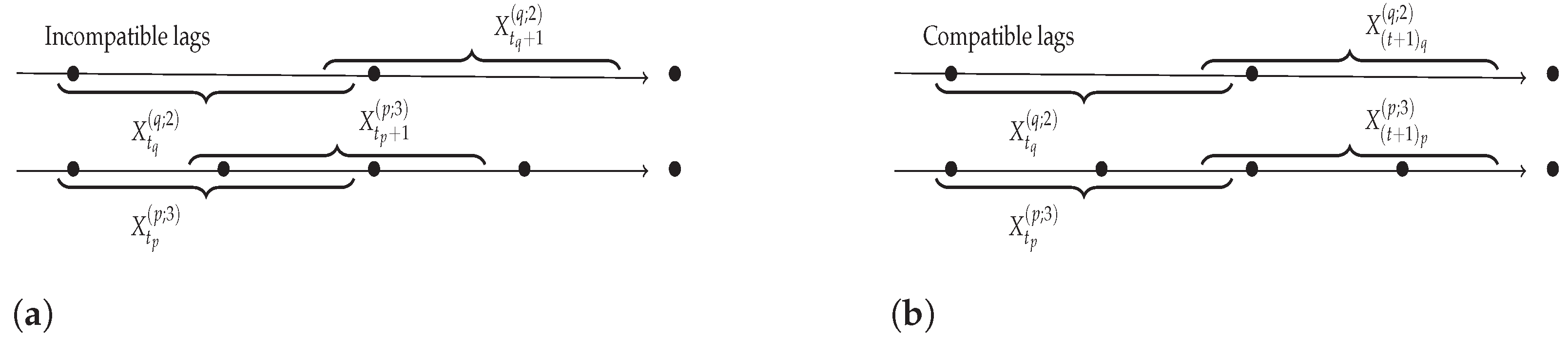
- We also show how this measure can be used for time series with different sampling rates;
- We finally combine these three ingredients in PC-like and FCI-like algorithms [9] to construct the summary causal graph from time series with equal or different sampling rates.
2. Related Work
3. Information Measures for Causal Discovery in Time Series
3.1. Causal Temporal Mutual Information
3.2. Entropy Reduction Principle
3.3. Conditional Causal Temporal Mutual Information
3.4. Estimation and Testing
3.5. Extension to Time Series with Different Sampling Rates
4. Causal Discovery Based on Causal Temporal Mutual Information
4.1. Without Hidden Common Causes
4.1.1. Skeleton Construction
4.1.2. Orientation
| Algorithm 1PCTMI. |
| X a d-dimensional time series of length T, the maximum number of lags, a significance threshold Form a complete undirected graph with d nodes n = 0 while there exists such that do for s.t. do for do for all subsets such that and ( or ) for all do append Sort by increasing order of y while is not empty do if and then Compute z the p-value of given by Equation (4) if test then Remove edge from n = n + 1 for each triple in , do apply PC-rule 0 while no more edges can be oriented do for each triple in , do apply PC-rules 1, 2, and 3 for each connected pair in do apply ER-rules 0 and 1 Return |
4.2. Extension to Hidden Common Causes
| Algorithm 2FCITMI. |
| Require:X a d-dimensional time series of length T, the maximum number of lags, a significance threshold Form a complete undirected graph with d nodes n = 0 while there exists such that do for s.t. do for do for all subsets such that and ( or ) for all do append Sort by increasing order of y while is not empty do if and then Compute z the p-value of given by Equation (4) if test then Remove edge from n = n + 1 for each triple in , do apply FCI-rule 0 using Possible-Dsep sets, remove edges using CTMI Reorient all edges as in for each triple in , do apply FCI-rule 0 while edges can be oriented do for each triple in , apply FCI-rules 1, 2, 3, 4, 8, 9, and 10 for each connected pair in , do apply ER-rules 0 and 1. Return |
5. Experiments
5.1. Methods and Their Use
5.2. Datasets
5.2.1. Simulated data
5.2.2. Real Data
5.3. Numerical Results
5.3.1. Simulated Data
5.3.2. Real Data
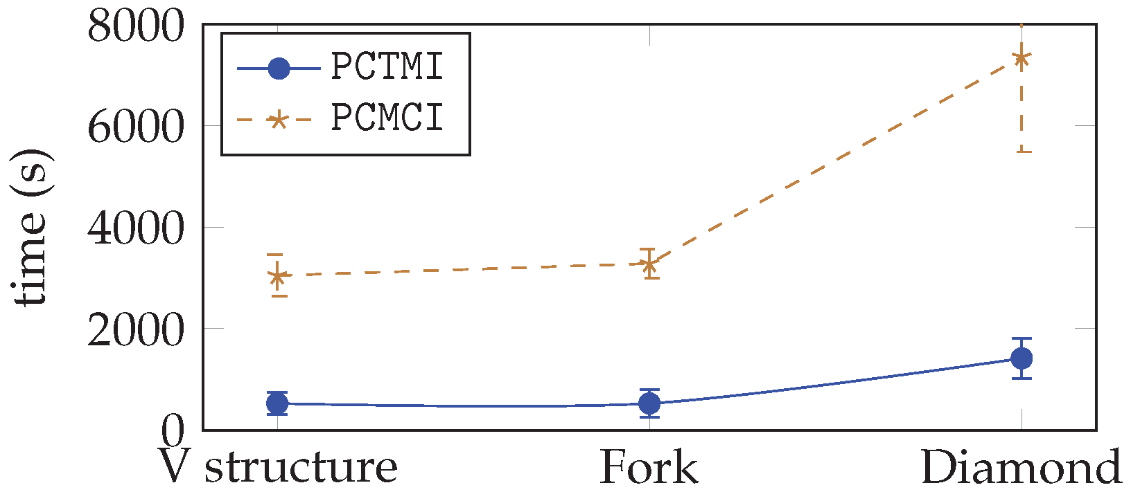
5.3.3. Complexity Analysis
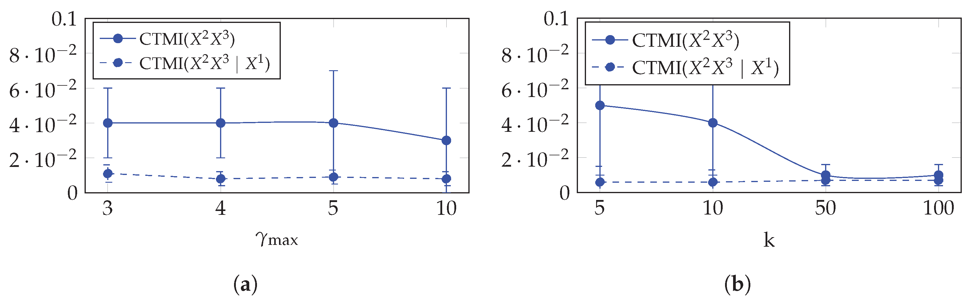
5.3.4. Hyperparameters’ Analysis
6. Discussion and Conclusions
Author Contributions
Funding
Institutional Review Board Statement
Informed Consent Statement
Data Availability Statement
Acknowledgments
Conflicts of Interest
References
- Assaad, C.K.; Devijver, E.; Gaussier, E. Survey and Evaluation of Causal Discovery Methods for Time Series. J. Artif. Intell. Res. 2022, 73, 767–819. [Google Scholar] [CrossRef]
- Wang, P.; Xu, J.; Ma, M.; Lin, W.; Pan, D.; Wang, Y.; Chen, P. CloudRanger: Root Cause Identification for Cloud Native Systems. In Proceedings of the 2018 18th IEEE/ACM International Symposium on Cluster, Cloud and Grid Computing (CCGrid ’18), Washington, DC, USA, 1–4 May 2018; pp. 492–502. [Google Scholar] [CrossRef]
- Wang, H.; Wu, Z.; Jiang, H.; Huang, Y.; Wang, J.; Kopru, S.; Xie, T. Groot: An Event-Graph-Based Approach for Root Cause Analysis in Industrial Settings. In Proceedings of the 2021 36th IEEE/ACM International Conference on Automated Software Engineering (ASE ’21), Melbourne, Australia, 15–19 November 2021; pp. 419–429. [Google Scholar] [CrossRef]
- Zhang, Y.; Guan, Z.; Qian, H.; Xu, L.; Liu, H.; Wen, Q.; Sun, L.; Jiang, J.; Fan, L.; Ke, M. CloudRCA: A Root Cause Analysis Framework for Cloud Computing Platforms. In Proceedings of the 30th ACM International Conference on Information and Knowledge Management, Association for Computing Machinery, Online, 1–5 November 2021; pp. 4373–4382. [Google Scholar]
- Granger, C. Investigating Causal Relations by Econometric Models and Cross-Spectral Methods. Econometrica 1969, 37, 424–438. [Google Scholar] [CrossRef]
- Peters, J.; Janzing, D.; Schölkopf, B. Causal Inference on Time Series using Restricted Structural Equation Models. In Proceedings of the Advances in Neural Information Processing Systems 26, Lake Tahoe, NV, USA, 5–10 December 2013; pp. 154–162. [Google Scholar]
- Runge, J.; Nowack, P.; Kretschmer, M.; Flaxman, S.; Sejdinovic, D. Detecting and quantifying causal associations in large nonlinear time series datasets. Sci. Adv. 2019, 5, eaau4996. [Google Scholar] [CrossRef] [PubMed]
- Nauta, M.; Bucur, D.; Seifert, C. Causal Discovery with Attention-Based Convolutional Neural Networks. Mach. Learn. Knowl. Extr. 2019, 1, 312–340. [Google Scholar] [CrossRef]
- Spirtes, P.; Glymour, C.; Scheines, R. Causation, Prediction, and Search, 2nd ed.; MIT Press: Cambridge, MA, USA, 2000. [Google Scholar]
- Granger, C.W.J. Time Series Analysis, Cointegration, and Applications. Am. Econ. Rev. 2004, 94, 421–425. [Google Scholar] [CrossRef]
- Chickering, D.M. Learning Equivalence Classes of Bayesian-Network Structures. J. Mach. Learn. Res. 2002, 2, 445–498. [Google Scholar] [CrossRef]
- Pamfil, R.; Sriwattanaworachai, N.; Desai, S.; Pilgerstorfer, P.; Georgatzis, K.; Beaumont, P.; Aragam, B. DYNOTEARS: Structure Learning from Time-Series Data. In Proceedings of the Twenty Third International Conference on Artificial Intelligence and Statistics, Online, 28 August 2020; Volume 108, pp. 1595–1605. [Google Scholar]
- Sun, J.; Taylor, D.; Bollt, E.M. Causal Network Inference by Optimal Causation Entropy. SIAM J. Appl. Dyn. Syst. 2015, 14, 73–106. [Google Scholar] [CrossRef]
- Entner, D.; Hoyer, P. On Causal Discovery from Time Series Data using FCI. In Proceedings of the 5th European Workshop on Probabilistic Graphical Models, PGM 2010, Helsinki, Filnland, 13–15 September 2010. [Google Scholar]
- Malinsky, D.; Spirtes, P. Causal Structure Learning from Multivariate Time Series in Settings with Unmeasured Confounding. In Proceedings of the 2018 ACM SIGKDD Workshop on Causal Disocvery, London, UK, 20 August 2018; Volume 92, pp. 23–47. [Google Scholar]
- Assaad, C.K.; Devijver, E.; Gaussier, E.; Ait-Bachir, A. A Mixed Noise and Constraint-Based Approach to Causal Inference in Time Series. In Machine Learning and Knowledge Discovery in Databases. Research Track, Proceedings of the Machine Learning and Knowledge Discovery in Databases, Bilbao, Spain, 13–17 September 2021; Springer International Publishing: Cham, Switzerland, 2021; pp. 453–468. [Google Scholar]
- Shannon, C.E. A Mathematical Theory of Communication. Bell Syst. Tech. J. 1948, 27, 379–423. [Google Scholar] [CrossRef]
- Affeldt, S.; Isambert, H. Robust Reconstruction of Causal Graphical Models Based on Conditional 2-point and 3-point Information. In Proceedings of the Thirty-First Conference on Uncertainty in Artificial Intelligence (UAI’15); Amsterdam, The Netherlands, 12–16 July 2015, AUAI Press: Amsterdam, The Netherlands, 2015. [Google Scholar]
- Galka, A.; Ozaki, T.; Bayard, J.B.; Yamashita, O. Whitening as a Tool for Estimating Mutual Information in Spatiotemporal Data Sets. J. Stat. Phys. 2006, 124, 1275–1315. [Google Scholar] [CrossRef]
- Schreiber, T. Measuring Information Transfer. Phys. Rev. Lett. 2000, 85, 461. [Google Scholar] [CrossRef] [PubMed]
- Marko, H. The Bidirectional Communication Theory—A Generalization of Information Theory. IEEE Trans. Commun. 1973, 21, 1345–1351. [Google Scholar] [CrossRef]
- Massey, J.L. Causality, feedback and directed information. In Proceedings of the International Symposium on Information Theory and Its Applications, Waikiki, HI, USA, 27–30 November 1990. [Google Scholar]
- Albers, D.J.; Hripcsak, G. Estimation of time-delayed mutual information and bias for irregularly and sparsely sampled time-series. Chaos Solitons Fractals 2012, 45, 853–860. [Google Scholar] [CrossRef] [PubMed]
- Suppes, P. A Probabilistic Theory of Causality; North-Holland Pub. Co.: Amsterdam, The Netherlands, 1970. [Google Scholar]
- Kraskov, A.; Stögbauer, H.; Grassberger, P. Estimating mutual information. Phys. Rev. E Stat. Nonlinear, Soft Matter Phys. 2004, 69 Pt 2, 066138. [Google Scholar] [CrossRef] [PubMed]
- Frenzel, S.; Pompe, B. Partial Mutual Information for Coupling Analysis of Multivariate Time Series. Phys. Rev. Lett. 2007, 99, 204101. [Google Scholar] [CrossRef] [PubMed]
- Runge, J. Conditional independence testing based on a nearest-neighbor estimator of conditional mutual information. In Proceedings of the Twenty-First International Conference on Artificial Intelligence and Statistics, Playa Blanca, Spain, 9 April 2018; Volume 84, pp. 938–947. [Google Scholar]
- Colombo, D.; Maathuis, M.H. Order-Independent Constraint-Based Causal Structure Learning. J. Mach. Learn. Res. 2014, 15, 3921–3962. [Google Scholar]
- Zhang, J. On the completeness of orientation rules for causal discovery in the presence of latent confounders and selection bias. Artif. Intell. 2008, 172, 1873–1896. [Google Scholar] [CrossRef]
- Smith, S.M.; Miller, K.L.; Khorshidi, G.S.; Webster, M.A.; Beckmann, C.F.; Nichols, T.E.; Ramsey, J.; Woolrich, M.W. Network modelling methods for FMRI. NeuroImage 2011, 54, 875–891. [Google Scholar] [CrossRef] [PubMed]


| V-Structure | Fork | Diamond |
|---|---|---|
 | 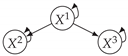 | 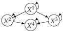 |
| 7ts2h |
|---|
 |
| PCTMI | PCMCI | TiMINo | VarLiNGAM | Dynotears | TCDF | MVGC | |
|---|---|---|---|---|---|---|---|
| V structure | |||||||
| Fork | |||||||
| Diamond |
| PCTMI | |
|---|---|
| V structure | |
| Fork | |
| Diamond |
| FCITMI | tsFCI | |
|---|---|---|
| 7ts2h |
| PCTMI | PCMCI | TiMINo | VarLiNGAM | Dynotears | TCDF | MVGC | |
|---|---|---|---|---|---|---|---|
| fMRI | |||||||
| IT |
| PCTMI | PCMCI | TiMINo | VarLiNGAM | MVGC | |
|---|---|---|---|---|---|
| Dataset 1 |  |  |  |  |  |
| Dataset 2 |  |  |  |  |  |
| Dataset 3 |  |  |  |  |  |
| Dataset 4 |  |  |  |  |  |
| Dataset 5 |  |  |  |  |  |
| Dataset 6 |  |  |  |  |  |
| Dataset 7 |  |  |  |  |  |
| Dataset 8 |  |  |  |  |  |
| Dataset 9 |  |  |  |  |  |
| Dataset 10 |  |  |  |  |  |
Publisher’s Note: MDPI stays neutral with regard to jurisdictional claims in published maps and institutional affiliations. |
© 2022 by the authors. Licensee MDPI, Basel, Switzerland. This article is an open access article distributed under the terms and conditions of the Creative Commons Attribution (CC BY) license (https://creativecommons.org/licenses/by/4.0/).
Share and Cite
Assaad, C.K.; Devijver, E.; Gaussier, E. Entropy-Based Discovery of Summary Causal Graphs in Time Series. Entropy 2022, 24, 1156. https://doi.org/10.3390/e24081156
Assaad CK, Devijver E, Gaussier E. Entropy-Based Discovery of Summary Causal Graphs in Time Series. Entropy. 2022; 24(8):1156. https://doi.org/10.3390/e24081156
Chicago/Turabian StyleAssaad, Charles K., Emilie Devijver, and Eric Gaussier. 2022. "Entropy-Based Discovery of Summary Causal Graphs in Time Series" Entropy 24, no. 8: 1156. https://doi.org/10.3390/e24081156
APA StyleAssaad, C. K., Devijver, E., & Gaussier, E. (2022). Entropy-Based Discovery of Summary Causal Graphs in Time Series. Entropy, 24(8), 1156. https://doi.org/10.3390/e24081156