Abstract
The problem addressed by dictionary learning (DL) is the representation of data as a sparse linear combination of columns of a matrix called dictionary. Both the dictionary and the sparse representations are learned from the data. We show how DL can be employed in the imputation of multivariate time series. We use a structured dictionary, which is comprised of one block for each time series and a common block for all the time series. The size of each block and the sparsity level of the representation are selected by using information theoretic criteria. The objective function used in learning is designed to minimize either the sum of the squared errors or the sum of the magnitudes of the errors. We propose dimensionality reduction techniques for the case of high-dimensional time series. For demonstrating how the new algorithms can be used in practical applications, we conduct a large set of experiments on five real-life data sets. The missing data (MD) are simulated according to various scenarios where both the percentage of MD and the length of the sequences of MD are considered. This allows us to identify the situations in which the novel DL-based methods are superior to the existing methods.
1. Introduction
1.1. Background
It is well-known from the classical literature on time series that a multivariate time series data set is obtained by measuring variables at time points . The observations are stored in a matrix with T rows and K columns. For ease of writing, we use the notation for this matrix. In our notation, the bold letters are used for vectors and matrices. Due to recent technological advances, both T and K are very large for the data sets that are collected nowadays. The massive amount of data poses difficulties for both the storage and the processing. Another challenge comes from the fact that some of the entries of the big matrix are missing. The data are incomplete for various reasons: malfunction of the sensors, problems with the transmission of the measurements between devices, or the fact that it is practically impossible to collect all the data (for example, this happens often in astronomy).
The conventional approach is to estimate the missing data and then to use the resulting complete data set in statistical inference. The estimation methods span a wide range from the simple ones that perform imputation for each time series individually by considering the mean or the median, or employ the last value carried forward or the next value carried backward, to the more advanced ones that involve the evaluation of the (Gaussian) likelihood, see for example [1].
In here we do not discuss the imputation methods that can be easily found in the time series textbooks, but we briefly present the newer methods that have been compared in [2]. For instance, we consider the method DynaMMO from [3], which is closer to the traditional methods in the sense that it uses a technique akin to the Kalman filter (see again [1]) to estimate the missing values. The other methods that we outline below are based on the decomposition of the matrix ; hence, it is not surprising that they have a certain relationship with the singular value decomposition (SVD). In fact, SVDImp from [4] explicitly uses the SVD factorization of the matrix , after replacing the missing values with the mean computed for the corresponding row. Note that the symbol denotes transposition. The most significant rows of are selected, where the value of is chosen empirically. Then the linear regression is used to express each row of as a linear combination of the most significant rows of . In this way, new estimates are obtained for the missing data, and the procedure above is applied again to the matrix that contains these imputed values. The iterations are continued until the change of the magnitudes of the imputed values between two consecutive iterations is smaller than a threshold selected by the user.
In [5], the imputation problem is formulated as a matrix completion problem. The obtained estimate has the same entries as at the locations for which the measurements are available. The matrix is found by solving a penalized least-squares problem whose expression contains a coefficient that balances the two terms involved: (i) half of the sum of the squares of the approximation errors, or equivalently (the notation stands for the Frobenius norm), and (ii) the sum of the singular values of , or equivalently the nuclear norm of . The solution is given by a soft-thresholded SVD of , where the soft threshold is . This suggests the name Soft-Impute of the method for which we use the acronym SoftImp. In SoftImp, the solutions are obtained in a computationally efficient manner for all the values of on a predefined grid. Another algorithm that solves the same penalized least-squares problem by computing the soft-thresholded SVD at each iteration is the Singular Value Thresholding (SVT) from [6]. A particular attribute of SVT is that it automatically finds the optimal rank of the estimated matrix.
An approximation of SVD, which is called centroid decomposition (CD), is employed in [7,8] for representing the matrix as , where and . Either interpolation or extrapolation is applied for estimating the missing entries of and then a vector is found such that the Euclidean norm is maximized. The vector is obtained and is further used to obtain the first column of , , and the first column of , . For a better understanding of why the method is named CD, we mention that is the first centroid vector. The “new” matrix is taken to be , and the algorithm continues until all K columns of and are obtained. Only the first columns are used to obtain the approximation of given by , and this approximation yields the estimates for the missing values. It is interesting that the selection of is performed by an entropy-based criterion. When CD is employed in time series recovery we call it CDRec (as in [2]).
Another imputation method is dubbed Grassmannian Rank-One Update Subspace Estimation (GROUSE), see for example [9,10]. The name comes from the set of all subspaces of of dimension that is called Grassmannian. It is evident that an element of the Grassmanian can be represented by any matrix with the property that , where denotes the identity matrix of appropriate dimension. GROUSE finds the matrix that minimizes the objective function , where is a diagonal matrix which has on the main diagonal ones on the locations corresponding to the data that are available for the jth column of and zeros otherwise. The presence of in the formula above shows that the algorithm can work directly with the columns of that have missing data. In fact, GROUSE optimizes the cost function by considering one column of at a time, and at each such step, the matrix is updated by adding a rank-one matrix to the matrix obtained at the previous step. Once the “final” is found at the last step, the incomplete columns are projected onto the low-rank subspace that was identified to complete the matrix.
In robust principal component analysis (RPCA), the data matrix (which is supposed to be complete) is represented as a low-rank matrix plus a sparse matrix [11]. Because the recovery of the low-rank matrix is computationally intensive, an efficient algorithm called Robust Orthogonal Subspace Learning (ROSL) was proposed in [12]. The algorithm was altered in [2] to be applied to an incomplete data matrix for estimating the missing values. We use the acronym ROSL for the version of the algorithm from [2].
The imputation method from [13] relies on the nonnegative matrix factorization (NMF) technique and, to be suitable for electricity consumption, uses temporal aggregates. The optimization problem solved by the algorithm proposed in [13] takes into consideration the correlation between time series. As in [2], we call this method temporal NMF (TeNMF). The matrix factorization is also used in [14], but in contrast to TeNMF, the entries of the two factor matrices are not constrained to be nonnegative. An important feature of the method is that the regularization term of the objective function takes explicitly into consideration the temporal structures, and this is why the method is termed Temporal Regularized Matrix Factorization (TRMF).
Another matrix factorization that can be instrumental in time series imputation is the one generated by dictionary learning (DL).
1.2. Organization of the Paper and the Main Contributions
In this article, we extend the DL-based solution for time series imputation which we proposed in our earlier work [15]. Our previous results from [15] consist of two imputation methods: DLU (for univariate time series) and DLM (for multivariate time series). However, because of the computational complexity, the original version of DLM can be utilized only when the number of the time series involved is very small. In contrast, the variants of DLM that we introduce in this study can be applied to data sets that contain tens of time series.
DLM is presented in Section 2.2 after briefly discussing the DL optimization problem in Section 2.1. An important characteristic of DLM is that it solves the optimization problem by minimizing the Frobenius norm of the errors. In many practical situations, the imputation should be performed to minimize the -norm of the errors and not the sum of the squared errors. In Section 3, we demonstrate how the optimization problem can be solved when the Frobenius norm is replaced with the sum of the magnitudes of errors. The method that involves the -norm is dubbed . Another characteristic of DLM (which is also inherited by ) is the use of a structured dictionary. In Section 4, we present the expressions of the IT criteria that are employed to select the size of the structured dictionary, the size for each of its blocks as well as the sparsity level of the representation. Section 5 is focused on the techniques that we propose for dimensionality reduction. It allows us to apply DLM and to data sets that comprise tens of time series with thousands of measurements. For demonstrating how the new algorithms can be used in practice, we conduct a large set of experiments with real-life data. The experimental settings are presented in Section 6, and the empirical results are discussed in Section 7. Section 8 concludes the paper.
Hence, the main contributions of this work are the following:
- A flexible approach that allows the user to choose the norm of the errors (Frobenius norm or -norm) minimized in the optimization problem.
- An automatic method for selecting the sparsity as well as the size for each block of the dictionary.
- The exemplification of two techniques for dimensionality reduction that enable DLM to impute values on multivariate time series for which K is large.
- An extensive empirical study which compares DLM with nine other imputation methods on data sets with various characteristics. On many of these data sets, DLM has the best performance among the considered methods when the missing data are simulated by sampling without replacement.
2. Dictionary Learning for Data Sets with Missing Values
2.1. Preliminaries
The DL problem is formulated as follows. Given N signals of length m that are grouped into the matrix , we approximate by the product , where is the dictionary, and its columns are usually named atoms. The Euclidean norm of each atom equals one. The matrix is sparse in the sense that each of its columns contains at most s non-zero entries, the parameter s being named sparsity level. We emphasize that both and are learned from the signals by solving the following optimization problem [16]:
the ℓ-th column of is denoted , and the j-th column of is denoted . The symbol represents the number of the non-zero entries for the vector in the argument.
The algorithm that solves the optimization problem in (1) is initialized with a dictionary , which is generally randomly generated. The user selects the number of iterations, and the following steps are executed at each iteration:
- (i)
- The current dictionary is used to find the matrix , which provides a representation for the signals in . This goal is achieved by employing the Orthogonal Matching Pursuit (OMP).
- (ii)
- The dictionary is updated by using the current sparse representation . This is performed by using the Approximate K-Singular Value Decomposition (AK-SVD) algorithm.
The two steps of the main algorithm are presented in [17].
There are other ways of posing the DL problem. For example, one may add a sparsity enhancing term to the objective and thus impose sparsity globally, not on each representation; thus, one can obtain a matrix that has around nonzeros without the explicit constraint that each of its columns has s nonzeros. A representative of this approach is [18]. Convolutional DL [19] does not split the time series into signals of size m, but works with a single long signal that is approximated as a linear combination of atoms of length m that may be placed at any position; the same atom can be used repeatedly. These approaches may provide more flexibility, but they require more fine tuning of the parameters and adaptation of dictionary size criteria. We prefer AK-SVD because it is one of the fastest DL-algorithms that have been proposed in the previous literature. Another important feature of the algorithm is its conceptual simplicity, which allows it to be easily modified for solving particular formulations of DL that appear in the context of imputation.
2.2. Optimization Problem for Incomplete Data: Formulation, Solution and Applications
When some of the entries of the matrix are missing, the optimization problem in (1) becomes [20]:
where is a mask matrix with the same size as . Its entries are equal to zero for the positions in that correspond to the missing data. All other entries of are equal to one. The operator ⊙ is the element-wise product. The role of is to guarantee that only the available data are used in learning. Note that the missing data are replaced with zeros in . For the optimization problem in (2), a specialized version of the AK-SVD algorithm is applied [16] [Section 5.9]; the representation matrix is found using OMP by ignoring the missing samples and working only with the present ones; the atom update formulas are simple adaptations of AK-SVD rules to the incomplete data case.
An important application of (2) consists of filling the gaps of an incomplete image and is called image inpainting. In the case of this application, the matrix is generated as follows (see, for example, [16] [Section 2.3.1]). A patch of pixels of size is selected from a random location in the image. Then its columns are stacked to generate the signal , which is a column of . The procedure continues until all N signals are produced. Obviously, it is not allowed to select the same patch twice, but it is highly recommended to select patches that overlap. In what concerns the sizes of the patches, the value is often used. Values such as and have also been used, but they are not commonly employed because of the increased computational burden. Once the dictionary is learned, the product yields an estimate of . Any missing pixel is obtained by averaging its values from all entries of where it appears. More details about image inpainting can be found in [21,22,23,24]. The use of the inpainting was extended from images to audio signals in [20,25].
Our main goal is to show how DL can be employed for estimating the values of the missing data in multivariate time series. As we have already pointed out, the use of DL in the imputation of time series was discussed in [15]. The approach adopted in the multivariate case should take into consideration the dynamic interrelationships between variables whose measurements collected at time points are stored in matrix . Suppose that some of the entries of are missing. As the positions of the missing data are not necessarily the same for all the time series, we use the symbol to denote the indexes of the measurements that are available for the k-th time series, where . Obviously, the set of indexes of missing data for the k-th time series is .
Let be one of the columns of the data matrix in which the missing data indexed by are replaced with zeros. We define a matrix as follows:
For an arbitrary vector , denotes the entries of the vector whose indexes belong to the set , where . The number of rows of the matrix is m, and its choice depends on the sampling period. The parameter h is called signal shift and controls the overlapping between the columns of , and the value of q is given by . It follows that the number of columns of the matrix is . Herein we take , which leads to and .
If , then is a missing value, and this will be represented as a zero-entry in . As there is an overlap between the columns of , the missing value leads to several zero-entries in . We collect all the values of these entries from and compute an estimate for by averaging them.
For example, suppose , which means that is missing. Then the matrix is given by:
In addition, the entries of the matrix are:
where . It results that the estimate of the missing value is computed by averaging the red-colored entries of , whose positions are the same as the positions of in . Thus, we obtain as:
This imputation method was introduced in [15]. As it can be easily seen from the description above, the method is suitable for univariate time series, and for this reason it is named DLU (see again Section 1.2). In the multivariate case, the data matrix is
where is made of data measured for the i-th time series for . In [15], it was pointed out that in the DLM algorithm designed for the multivariate case, a structured dictionary should be used:
where and . The dictionary is dedicated to the representation of the i-th time series, while is common for all time series. It follows that the number of atoms used in the representation of each time series is . The values of and as well as the sparsity level s are selected by using information theoretic (IT) criteria [26]. The main advantage is that the procedure for choosing the triple does not rely on prior knowledge. We take the sizes of dictionaries to be equal to simplify the decision process, but also to use similar representation power for all times series (or groups of time series, as we will see later).
We mention that there are many DL algorithms that choose the size of the dictionary. Most of them are based on heuristics, such as, for example, growing a small dictionary [27] or removing atoms from a large one [28], with the general purpose of achieving parsimony. Other approaches are more principled, using Bayesian learning [29] or an Indian Buffet Process [30]. We have used IT criteria in [26], where we also presented a more detailed view of the topic, including bibliographic references. IT criteria offer a sound evaluation of the trade-off between dictionary size and representation error.
Next we show how the new algorithm can be devised.
3. : DL-Algorithm for Incomplete Data (with -Norm)
We solve the -norm version of (2):
where for a matrix we denote , the -equivalent of the Frobenius norm. So, the aim of (5) is to optimize the sparse -norm representation of the signals, whereas (2) targets the -norm.
We modify the algorithm proposed in [31] such that it is suitable for the missing data case. The algorithm is an adaptation of the AK-SVD [17] idea and consists of iterations containing the usual two steps, sparse representation and dictionary update, as described in Section 2.1. We will next discuss these steps in detail.
3.1. -Norm OMP with Missing Data
We present a -norm version of the greedy approach whose most prominent representative is OMP [32]. It is enough to consider a single signal , for which we have to minimize , where is the given dictionary, must have at most s nonzero elements, and is the mask whose entries are zeros and ones.
We denote () the vector that results from by keeping only the elements that correspond to nonzero values in . Similarly, is the matrix obtained from by keeping only the rows corresponding to nonzero values in . We are thus left with the problem , which is a usual -norm sparse representation problem for which the algorithm was described in [31].
For the sake of completeness, we revisit the main operations here. The algorithm has s steps. Denoting the representation at the beginning of the current step and the current residual, the next selected atom is that for which
is attained. Thus, we follow the idea of finding the atom with the best projection on the residual.
The problem (we lighten the notation for the sake of simplicity) can be easily solved. It is not only convex, but its solution can be found by inspection [33]. Denote , for . Denote the vector containing the elements of sorted increasingly and the permutation for which . Denote . The desired minimum is , where the index k is the largest for which
So, finding the solution essentially requires only a sort operation. Moreover, in solving (6), some atoms can be ignored if their scalar product (usual orthogonal projection) with the residual is small.
Once the current atom has been found, it is added to the support, and the optimal -norm representation with that support is computed. This is a convex problem and can be solved by several nonlinear optimization algorithms (we have used a few coordinate descent iterations). Moreover, a good initialization is available in the representation at the previous step. (In OMP, these operations correspond to finding a least-squares solution.)
3.2. Dictionary Update with Missing Data in the -Norm
The update stage of AK-SVD optimizes the atoms one by one, also updating the coefficients of the corresponding representations. Denote the current atom and the set of signals where this atom contributes to the representation. Denote the current residual and
the error without the contribution of , keeping only the columns where appears in the representation.
With lighter notation, namely for the current atom, for the vector of its nonzero representation coefficients and for the mask (even though the signals where is not used are removed), the atom update problem becomes
Denoting the indexes of available data, the problem can be written as
The minimization can be performed on each separately and has the form , where and are vectors that can be easily built. We thus end up with a problem similar to that described after (6).
Keeping the updated atom fixed, we can now optimize the associated representation coefficients by solving
which can be written
like (7) was written as (8). The problem is separable on each and can be solved as above.
We note that we use the same basic algorithm in the -norm OMP, atom and representation update. The approach can be extended to -norms, with , transforming the -norm AK-SVD from [31] to the missing data case, similarly to the transformations described in this section.
4. Information Theoretic Criteria
We have already mentioned in Section 2.2 that we employ IT criteria for selecting the triple . More precisely, the criteria that we use are derived from the well-known Bayesian information criterion (BIC) [34]. For evaluating the complexity of the model, we need to calculate the number of parameters (NoP). We have that . The first term is given by the number of the non-zero entries for the representation matrix , which is estimated from the available data by solving the optimization problem (2). The second term is equal to the number of the entries of the estimated dictionary ; for each column of , we count entries (and not m entries) because each column is constrained to have the Euclidean norm equal to one. Furthermore, we define the matrix of residuals . Note that the residuals located at the positions corresponding to the missing data are forced to be zero. With the understanding that is the number of the entries of that are equal to one, the expression of the first IT criterion that we employ is:
where denotes the natural logarithm. This criterion was proposed in [15], where its “extended” variant was also used (see [26,35]):
However, because of the way in which they have been derived, the formulas in (9) and (10) can only be used when and are outputs of the DLM algorithm. When the estimation is performed by applying the algorithm from Section 3, we employ the following formula for BIC:
The expression above is based on the criterion obtained in [31] for signals in additive Laplacian noise and is altered to be suitable for the missing data case. Its “extended” variant is easily constructed by adding the term to the expression above (see again [31]).
For clarifying the notation, we mention that when we write DLM+BIC, it means that the criterion in (9) is applied for model selection. At the same time, DLM1+BIC involves the criterion from (11). A similar convention is used for the “extended” criteria.
Whenever DLM is applied to multivariate time series with missing values, 10 random initializations of the dictionary are considered. For each initialization, 50 iterations of the two-step algorithm that involves OMP and AK-SVD for incomplete data are executed for each possible combination of , and s. Then the triple (, , s) which minimizes BIC/EBIC is selected. The procedure is the same when is used instead of DLM.
5. Dimensionality Reduction
5.1. Dimensionality Reduction via Clustering
When K is large, we group the time series to reduce the dimensionality. For exemplification, we refer to the particular case in which K is an even number, and the time series are clustered into two groups such that each group contains columns of . The set of the indexes of the time series that belong to the first group is , whereas the set of the indexes corresponding to the second group is . It is evident that and . Furthermore, we re-arrange the columns of the matrix into the matrix as follows:
The newly obtained matrix is regarded as a multivariate time series that contains time series observed at time points , where . Hence, the data matrix used by the DL algorithm (see (3)) has the expression where, for , is constructed from the entries of the i-th column of as in Section 2.2. According to the convention from (4), the structure of the dictionary is given by . It follows that the block is for the time series in group , the block is for the time series in group and the block is common for all the time series. The estimation of the missing values is performed as it was described in the previous sections.
5.2. Time Series Grouping
When deciding what time series to assign to the group , we should take into consideration that all these time series are represented by using atoms from the same blocks: and . Hence, it is desirable (i) to minimize the overlap of the sequences of missing data for the columns of that belong to , and (ii) to maximize the linear dependence between any two time series in . Because it is non-trivial to combine the two requirements, we first focused on the condition (i). After some preliminary experiments, we came to the conclusion that the approach does not lead to good results. Then we investigated more carefully the condition (ii). The result of this investigation is the heuristic for cluster selection that we present below and which is based on the evaluation of the absolute value of the Pearson correlation between the pairs of columns of the matrix .
For ease of exposition, we introduce the following notation. If is symmetric, then , where is the magnitude of the entry of located at the intersection of i-th row and the j-th column. Let be the matrix of the pairwise correlations between the columns of . For a subset whose cardinality equals , we take to be the block of that corresponds to the rows and the columns indexed by . Then we select as follows:
We note that the cardinality of is also . The formula implies that we find with the property that the sum of the absolute pairwise correlations of the time series in cluster is as close as possible to the sum of the absolute pairwise correlations of the time series in cluster plus the sum of the absolute correlations of the pairs that contain a time series from and a time series from . Remark that, in the particular case when the correlations for all the pairs that contain a time series from and a time series from are zero, the sum of the absolute pairwise correlations of the time series in cluster are approximately equal to the sum of the absolute pairwise correlations of the time series in cluster . This approach has two limitations: (i) it can be applied only when the number of groups is two, and (ii) the computational burden is too high when K is large.
An alternative solution is a greedy algorithm which can be employed when the number of groups, , is greater than two. For simplicity, we assume that K is a multiple integer of . The algorithm constructs the groups as follows. Initially, the two time series that have the largest absolute correlation are included in the first group . In other words, we take
and then . At the next step, it is included in the time series that increases the sum of the absolute correlations in the group the most:
and becomes . In general, after it was decided that , where , the th time series is selected as follows:
Once the first cluster is built, the second one is initialized with the two time series from that have the largest absolute correlation, and the steps described above are applied for obtaining the second cluster. The procedure continues until groups are produced. The last group results automatically.
6. Experimental Settings
6.1. Simulation of the Missing Data
When we conduct experiments on a real-life multivariate time series , we randomly select the positions of the missing data. The selection is performed such that the number of missing data, , is the same for each of the K time series. Hence, all the sets have the same cardinality. It follows that the percentage of missing data is
for each time series. In our experiments, we consider , , and .
The indexes of the missing data for a particular time series are independent of the positions of the missing data in the other time series from the same data set. They are selected by either sampling without replacement integers from the set or by using the Polya urn model (with finite memory), which was introduced in [36]. The Polya urn model is well-known, and it was employed in various applications. Some of these applications are: modeling of the communication channels [36,37,38,39], image segmentation [40] and modeling of epidemics on networks [41]. In [15], we have proposed the use of the Polya urn model for simulating the missing data in time series.
In the Polya model, the urn initially contains R red balls and S black balls (). At each time moment , a ball is drawn from the urn and, after each draw, balls of the same color as the drawn ball are returned to the urn. We take . More details about the selection of are provided below after the presentation of the most important properties of the model. Since we want the model to have finite memory, the experiment is performed as described above only for , where the parameter M is a positive integer (see the discussion in [36]). At each time moment , a ball is drawn from the urn and, after each draw, two operations are executed: (i) balls of the same color as the drawn ball are returned to the urn and (ii) balls of the same color as the ball picked at time are removed from the urn.
A sequence of random variables is defined as follows: if the ball drawn at time t is red and if the ball drawn at time t is black. It was proven in [36,39] that the sequence is a Markov process of order M. For , let denote the state . The Polya urn model has the remarkable property that the probability of having after the state was observed depends on the number of ones in , but not on their locations. We mention that in our settings.
The indexes of the missing data correspond to the positions of ones in the sequence . It is known that , where the symbol denotes probability. In our simulations, R and S are chosen such that . According to [39], the correlation is equal to , where and . This property allows us to simulate bursts of missing data by taking . Obviously, this is different from the situation when the sampling without replacement is applied and when it is more likely to have isolated missing data. At the same time, the simulation of the missing data by using the Polya urn model is different from the approach in [2], where blocks of missing data are considered.
6.2. Data Pre-Processing
After the missing values are simulated, each time series is decomposed into trend, seasonal component and remainder. Then the DLM imputation method is applied on the matrix of the remainder components. For each time series, both the trend and the seasonal components are added to the estimates produced by DLM to obtain the estimates for the missing data.
The decomposition uses the implementation for the R package imputeTS [42,43], which is available at https://github.com/SteffenMoritz/imputeTS/blob/master/R/na_seadec.R (accessed on 28 February 2022). The implementation returns a specific output when it cannot detect a seasonal pattern for the analyzed time series. From the package imputeTS, we only use the decomposition technique and not the imputation methods because all the imputation methods are designed for univariate time series; thus they are sub-optimal for the multivariate case.
6.3. Performance Evaluation
Let be a column of the data matrix . We collect in the vector the entries of the time series that are indexed by the elements of the set . With the convention that is the vector of estimates produced by DLM for the missing values of , we calculate the following normalized error:
The normalized errors are computed similarly for the estimates yielded by the imputation methods from [2]. To rank the methods, we calculate scores as follows. For each time series , the imputation method that achieves the minimum normalized error yields two points, the method that leads to the second smallest normalized error yields one point, and all other methods yield zero points. The number of points accumulated by each method from the experiment with all time series in are divided by to ensure that the scores take values in the interval .
When the imputation is performed by using , the expression in (14) is replaced with
and the scores are calculated as explained above.
In the empirical comparison of the methods, we have used the code available at https://github.com/eXascaleInfolab/bench-vldb20.git (accessed on 3 October 2021) for the imputation methods that have been assessed in [2]. Short descriptions of these methods have been given in Section 1.1.
In the next section, we present the results obtained by DLM on five data sets that have been also used in [2]. For the sake of conciseness, we report the scores for only for three data sets. The experimental results can be reproduced by using the Matlab code available at https://www.stat.auckland.ac.nz/%7Ecgiu216/PUBLICATIONS.htm (accessed on 17 June 2022).
7. Experimental Results
7.1. Climate Time Series (K = 10, T = 5000)
The data set comprises monthly climate measurements that have been recorded at various locations in North America from 1990 to 2002. We do not transform the time series with the method from Section 6.2 because it does not improve the quality of the imputation. As K is relatively small, we cluster the time series into groups that are found by using (12): and . It is interesting that the rule in (12) yields the same grouping for all percentages of the missing data, for both sampling without replacement and for the Polya model.
Since the data are sampled monthly, it is natural to take the signal length . We have , and for each value of , we take . Observe that , and it denotes the size of the block of the structured dictionary which contains atoms that are common for all time series. The sparsity level s is selected from the set . It follows that the total number of triples that we consider is 18.
We compute the normalized errors (see Table A1, Table A2, Table A3, Table A4, Table A5, Table A6, Table A7 and Table A8 in Appendix A.1.1), which lead to the scores shown in Figure 1. From the plot in the left panel of the figure, it is evident that both DLM+BIC and DLM+EBIC work better than other methods when the missing data are simulated by sampling without replacement. The method DLM+BIC is slightly superior to DLM+EBIC for all missing percentages, except for . In the right panel of the figure, where the Polya urn model is employed for simulating the missing data, we observe the following: the method DynaMMo is ranked the best for all missing percentages, except for , where DLM+BIC works better than DynaMMo. In Figure 2, we can see that DLM1+BIC and DLM1+EBIC are also very good when sampling without replacement is employed, but their performance diminishes in the case of the Polya model (for more details, see Table A9, Table A10, Table A11, Table A12, Table A13, Table A14, Table A15 and Table A16 in Appendix A.1.2).
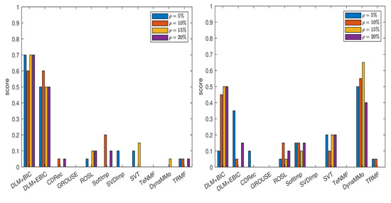
Figure 1.
Scores for various imputation methods applied to the Climate time series: The missing data are simulated by sampling without replacement (left panel) and by using the Polya model (right panel). Note that the DLM algorithm is used.
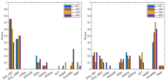
Figure 2.
Scores for various imputation methods applied to the Climate time series: The missing data are simulated by sampling without replacement (left panel) and by using the Polya model (right panel). Note that the algorithm is used.
7.2. Meteoswiss Time Series (K = 10, T = 10,000)
The measurements represent weather data collected in Swiss cities from 1980 to 2018. After simulating the missing data, we remove both the trend and the seasonal components for each time series (see Section 6.2). The transformed time series are clustered into groups as follows: and (see (12)).
As the time interval between successive observations of these time series is 10 min, the most suitable value for m would be (which corresponds to 24 h), but this makes the computational complexity too high. For keeping the computational burden at a reasonable level, we conduct experiments for three different values of m: , and . Note that each value of m corresponds to a time interval (in hours) that is a divisor of 24. For each value of m, is selected from the set and for each value of , we have that . The sparsity level s is chosen from the set . We use these settings for the case when the missing data are generated by sampling without replacement and . The results can be found in Table A17. It can be easily noticed that both DLM+BIC and DLM+EBIC yield very good results for all values of m.
Taking into consideration these results, we further conduct the experiments for all cases of missing data simulations by setting and . Hence, we have six candidates for . The grouping for which is employed. The results are reported in Table A18, Table A19, Table A20, Table A21, Table A22, Table A23, Table A24 and Table A25, in Appendix A.2.1, and in Figure 3. Both DLM+BIC and DLM+EBIC have outstanding performance for sampling without replacement, and they are very good when the Polya model is used. In the latter case, DLM+BIC is less successful when . According to the scores shown in Figure 4, which are based on Table A26, Table A27, Table A28, Table A29, Table A30, Table A31, Table A32 and Table A33 (see Appendix A.2.2), the ranking of the imputation methods does not change significantly when the algorithm DLM is replaced with .
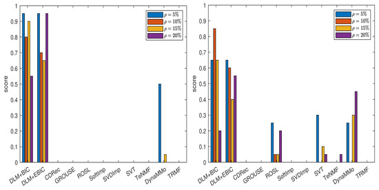
Figure 3.
Scores for various imputation methods applied to the MeteoSwiss time series: The missing data are simulated by sampling without replacement (left panel) and by using the Polya model (right panel). Note that the DLM algorithm is used.
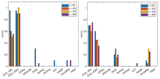
Figure 4.
Scores for various imputation methods applied to the MeteoSwiss time series: The missing data are simulated by sampling without replacement (left panel) and by using the Polya model (right panel). Note that the algorithm is used.
7.3. BAFU Time Series (K = 10, T = 50,000)
These are water discharge time series recorded by BAFU (BundesAmt Für Umwelt - Swiss Federal Office for the Environment) on Swiss rivers from 2010 to 2015. We do not remove the seasonality from the simulated incomplete time series because the method from [42] does not detect seasonal components for 3 out of 10 time series. Hence, the imputation is performed on the original time series. The grouping and is used to cluster the time series into groups when the missing data are simulated by sampling without replacement (for all missing percentages) or by the Polya model with . For the other three cases of missing data simulations, the grouping and is applied.
Relying on some of the empirical observations that we made for the MeteoSwiss time series and taking into consideration the fact that the sampling period for the BAFU time series is equal to 30 min, we set (which corresponds to a time interval of 6 h). The possible values for and are calculated by using the same formulas as in the experiments with climate and MeteoSwiss time series. In those experiments, we have noticed that the small values are preferred for the sparsity level, hence we take . This implies that the number of candidates for is the same as in the case of MeteoSwiss time series.
The normalized errors for this data set are given in Appendix A.3 (see Table A34, Table A35, Table A36, Table A37, Table A38, Table A39, Table A40 and Table A41). In Figure 5, we show the scores computed for various imputation methods. From the left panel of the figure, it is clear that both DLM+BIC and DLM+EBIC are the best for , where their scores are approximately one. The imputation method DLM+BIC does not work as well as DLM+EBIC when the percentage of the missing data is . In the right panel of the figure, we observe that both DLM+BIC and DLM+EBIC have modest performance when the missing data are simulated by the Polya model. In this case, DynaMMo and ROSL are the winners.
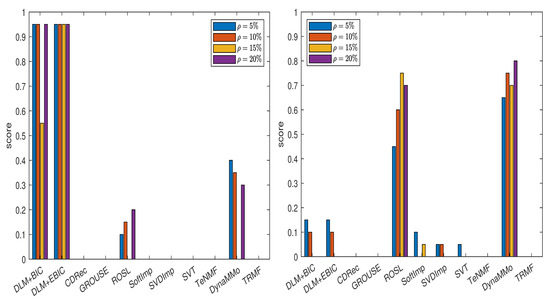
Figure 5.
Scores for various imputation methods applied to the BAFU time series: The missing data are simulated by sampling without replacement (left panel) and by using the Polya model (right panel).
7.4. Temperature Time Series (K = 50, T = 5000)
The data set contains average daily temperatures recorded at various sites in China from 1960 to 2012. After removing the trend and the seasonal components from all 50 time series with simulated missing data, we cluster them by applying the greedy algorithm which was introduced in Section 5.2. The resulting groups of time series are listed in Table A42 (see Appendix A.4). Note that the total number of groups is , and there are 10 time series in each group. It is interesting that the way in which the time series are assigned to the clusters depends very much on the method employed for simulating the missing data and on the percentage of missing data.
Mainly based on the lessons learned from the experiments with the data sets that have been analyzed in the previous sections, we have decided to take the signal length . We opt for relatively small values for , thus is selected from the set . For , we have that , which means that all the atoms are common for all the time series, and atoms that are specific for a certain group do not exist. For the other two values of , we allow to be selected from the set . The sparsity level s is selected from the set . Simple calculations lead to the conclusion that the total number of triples equals 10.
The normalized errors from Table A43, Table A44, Table A45, Table A46, Table A47, Table A48, Table A49 and Table A50 (see Appendix A.4) lead to the scores displayed in Figure 6. For the case of sampling without replacement, DLM+BIC, DLM+EBIC and ROSL have similar performance, and they are followed by CDRec. It is interesting that although SVT has a very modest rank when the percentage of the missing data is small, it becomes superior to all other methods when . As we have already observed for the BAFU time series, DLM+BIC and DLM+EBIC are not well ranked when the data are simulated by the Polya model. The difference compared with the results for the BAFU time series comes from the fact that ROSL and DynaMMo are not clear winners. This time, ROSL and CDRec are better than the other competitors. Similar to the case when the missing data are simulated by sampling without replacement, SVT outperforms all other imputation methods when .
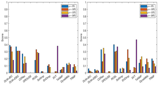
Figure 6.
Scores for various imputation methods applied to the Temperature time series: The missing data are simulated by sampling without replacement (left panel) and by using the Polya model (right panel).
7.5. Air Time Series (K = 10, T = 1000)
The data set comprises hourly sampled air quality measurements that have been recorded at monitoring stations in China from 2014 to 2015. For the case when the missing data are simulated by sampling without replacement (with ) and the Polya model (with ), the groups produced by the criterion in (12) are and . For the other two cases of missing data simulations, the clustering is: and . We do not remove the trend and seasonal components since, for each missing data simulation, the seasonal patterns are not detected in more than half of the time series.
We have applied DLM and algorithms on this data set. In both cases, we take the signal length because we analyze hourly data. The parameter is selected from the set . For each value of , we have that . The sparsity level s is selected from the set .
In Figure 7, we show the scores obtained by various imputation methods when the DLM algorithm is applied, and the normalized errors are computed with the formula from (14), see also Table A51, Table A52, Table A53, Table A54, Table A55, Table A56, Table A57 and Table A58 in Appendix A.5.1. It is evident that both DLM+BIC and DLM+EBIC have better performance when sampling without replacement is employed to simulate the missing data. SVT is clearly the best method for both cases of missing data simulations and for all percentages . The ranking of the imputation methods is the same in Figure 8, where the scores have been calculated by using (15), see Table A59, Table A60, Table A61, Table A62, Table A63, Table A64, Table A65 and Table A66 in Appendix A.5.2. An important difference between the two figures is that and the corresponding IT criteria are employed in Figure 8.
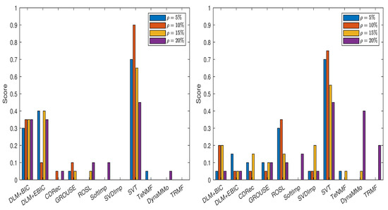
Figure 7.
Scores for various imputation methods applied to the Air time series: The missing data are simulated by sampling without replacement (left panel) and by using the Polya model (right panel). Note that the DLM algorithm is used.
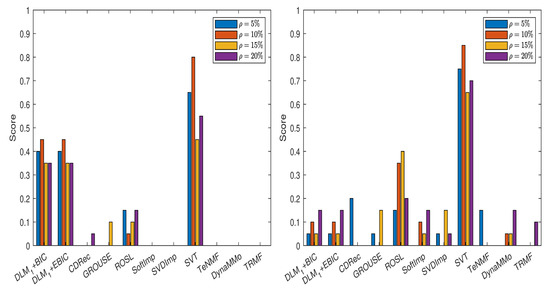
Figure 8.
Scores for various imputation methods applied to the Air time series: The missing data are simulated by sampling without replacement (left panel) and by using the Polya model (right panel). Note that the algorithm is used.
8. Final Remarks
In this work, we have exemplified how two techniques for dimensionality reduction can be employed for extending the use of the DLM algorithm to data sets that contain tens of time series. It remains to be investigated by the future research how the previous results on time series clustering can be utilized for grouping the time series and finding the number of groups (see, for example [44], for the definition of a metric that evaluates the dissimilarity between two time series). We have also derived the novel algorithm and the corresponding BIC and EBIC criteria. We have conducted a large set of experiments for comparing DLM and with nine algorithms that represent the state-of-the-art in the multivariate time series imputation.
Our empirical study confirms a fact already observed in the previous literature: There is no imputation method which always yields the best results. Although not always the best, our method clearly outperforms the other studied methods for some missing data models. So, it appears to be a useful addition to the existing methods. DLM tends to work better when the missing data are isolated (see the results for simulation by sampling without replacement) than in the case when the sequences of missing data are long (see the results for simulation by using the Polya model).
Both BIC and EBIC are effective in selecting the best structure of the dictionary and the sparsity. It is interesting that small values are chosen for the sparsity s, and this supports the idea that sparse models are appropriate for the multivariate time series. The values selected for are also relatively small. Recall that equals the number of atoms used in the representation of a specific time series (or a group of time series) plus the number of atoms that are common for all the time series in the data set.
Our imputation method can also be applied when the percentage of the missing data is not the same for all the time series in the data set. Based on the experimental results, it is easy to see that the percentage of missing data does not have an important influence on how DLM is ranked in comparison with other methods; thus we expect the same to be true when the number of missing data varies across the time series.
Author Contributions
Conceptualization, X.Z., B.D. and C.D.G.; methodology, X.Z., B.D. and C.D.G.; software, X.Z., B.D. and C.D.G.; validation, X.Z.; investigation, X.Z.; data curation, X.Z.; writing—original draft preparation, X.Z., B.D. and C.D.G.; writing—review and editing, X.Z., B.D., J.L. and C.D.G.; supervision, J.L. and C.D.G.; project administration, C.D.G. All authors have read and agreed to the published version of the manuscript.
Funding
B.D. was supported in part by a grant of the Ministry of Research, Innovation and Digitization, CNCS-UEFISCDI, project number PN-III-P4-PCE-2021-0154, within PNCDI III.
Data Availability Statement
Not applicable.
Acknowledgments
X.Z. would like to thank to Mourad Khayati from Department of Computer Science of the University of Fribourg, Switzerland for numerous hints on how to use the data and the code from https://github.com/eXascaleInfolab/bench-vldb20.git (accessed on 3 October 2021).
Conflicts of Interest
The authors declare no conflict of interest.
Appendix A
The tables below contain the normalized errors (see (14) and (15)) for the imputation methods that are assessed in this work. Note that the errors are computed for each time series in the data sets used in the empirical study. For each row in the tables, the best result is written in red and the second best result is written with bold font. For the methods DLM and , we also show the values of the triple (, , s) selected by BIC (see (9) and (11)) and EBIC (10). In the caption of each table, we provide information about the missing data: how they have been simulated and what is the value of (13). The only exception is Table A42 in Appendix A.4, which does not contain normalized errors, but shows the clustering of the time series.
Appendix A.1. Climate Time Series: Numerical Results
Appendix A.1.1. Results Obtained by Using DLM

Table A1.
Climate time series: Sampling without replacement ().
Table A1.
Climate time series: Sampling without replacement ().
| Time | DLM+BIC | DLM+EBIC | CDRec | GROUSE | ROSL | SoftImp | SVDImp | SVT | TeNMF | DynaMMo | TRMF |
|---|---|---|---|---|---|---|---|---|---|---|---|
| Series | = 240 | = 240 | |||||||||
| s = 2 | s = 2 | ||||||||||
| = 60 | = 180 | ||||||||||
| TS1 | 0.2206 | 0.9076 | 0.9206 | 1.1368 | 0.8791 | 0.8968 | 0.7794 | 0.9739 | 0.5496 | 0.8835 | |
| TS2 | 0.3859 | 0.6436 | 0.7692 | 0.7993 | 0.6225 | 0.6357 | 0.6140 | 0.6931 | 0.5437 | 0.6271 | |
| TS3 | 0.4527 | 0.9099 | 0.9346 | 0.8571 | 0.8732 | 0.8811 | 0.7824 | 0.8789 | 0.7286 | 0.8764 | |
| TS4 | 0.3806 | 0.9901 | 1.5210 | 1.0613 | 1.0005 | 1.0104 | 0.8415 | 0.9580 | 0.8624 | 1.0043 | |
| TS5 | 0.5997 | 0.6453 | 0.5979 | 0.7721 | 0.5862 | 0.5918 | 0.5597 | 0.5723 | 0.6048 | 0.5894 | |
| TS6 | 0.4955 | 0.6212 | 0.7566 | 0.5856 | 0.6037 | 0.6057 | 0.6812 | 0.6690 | 0.5529 | 0.6027 | |
| TS7 | 0.1928 | 0.6914 | 0.8858 | 0.7510 | 0.6683 | 0.6746 | 0.7331 | 1.0271 | 0.5201 | 0.6696 | |
| TS8 | 0.7010 | 0.7225 | 0.6346 | 0.7127 | 0.6369 | 0.6260 | 0.6252 | 0.6748 | 0.6424 | 0.6557 | |
| TS9 | 0.4232 | 0.9046 | 1.0713 | 0.9132 | 0.9305 | 0.9432 | 0.8629 | 1.0128 | 0.7983 | 0.9340 | |
| TS10 | 0.4963 | 0.7300 | 0.9366 | 0.8476 | 0.7216 | 0.7288 | 0.7219 | 1.1201 | 0.6585 | 0.7245 |
Table A2.
Climate time series: Sampling without replacement ().
Table A2.
Climate time series: Sampling without replacement ().
| Time | DLM+BIC | DLM+EBIC | CDRec | GROUSE | ROSL | SoftImp | SVDImp | SVT | TeNMF | DynaMMo | TRMF |
|---|---|---|---|---|---|---|---|---|---|---|---|
| Series | = 240 | = 240 | |||||||||
| s = 2 | s = 2 | ||||||||||
| = 60 | = 180 | ||||||||||
| TS1 | 0.3079 | 0.8854 | 0.9501 | 1.1632 | 0.8625 | 0.8793 | 0.7762 | 0.9942 | 0.5658 | 0.8676 | |
| TS2 | 0.3910 | 0.6454 | 0.8826 | 0.8076 | 0.6152 | 0.6312 | 0.6144 | 0.7761 | 0.5334 | 0.6226 | |
| TS3 | 0.4310 | 1.0124 | 0.9482 | 0.8484 | 0.9483 | 0.9636 | 0.7913 | 0.9159 | 0.7569 | 0.9514 | |
| TS4 | 0.3739 | 0.9442 | 1.2165 | 1.1301 | 0.9557 | 0.9660 | 0.8399 | 1.1305 | 0.8120 | 0.9574 | |
| TS5 | 0.6285 | 0.6536 | 0.5630 | 0.7562 | 0.5655 | 0.5552 | 0.5575 | 0.5868 | 0.5659 | 0.5763 | |
| TS6 | 0.5295 | 0.6570 | 1.0571 | 0.6188 | 0.6430 | 0.6481 | 0.6910 | 0.6838 | 0.5787 | 0.6439 | |
| TS7 | 0.1716 | 0.7024 | 0.8766 | 0.7107 | 0.6760 | 0.6866 | 0.7225 | 1.0463 | 0.5045 | 0.6772 | |
| TS8 | 0.7443 | 0.7381 | 0.7141 | 0.6395 | 0.6299 | 0.6344 | 0.6453 | 0.6517 | 0.6434 | 0.6321 | |
| TS9 | 0.4478 | 0.9088 | 1.0934 | 0.9006 | 0.9515 | 0.9659 | 0.8561 | 1.0037 | 0.7834 | 0.9546 | |
| TS10 | 0.4863 | 0.7862 | 0.9547 | 0.7982 | 0.7744 | 0.7803 | 0.7735 | 1.2519 | 0.7048 | 0.7760 |
Table A3.
Climate time series: Sampling without replacement ().
Table A3.
Climate time series: Sampling without replacement ().
| Time | DLM+BIC | DLM+EBIC | CDRec | GROUSE | ROSL | SoftImp | SVDImp | SVT | TeNMF | DynaMMo | TRMF |
|---|---|---|---|---|---|---|---|---|---|---|---|
| Series | = 240 | = 240 | |||||||||
| s = 2 | s = 2 | ||||||||||
| = 60 | = 180 | ||||||||||
| TS1 | 0.2636 | 0.9645 | 1.0027 | 1.1502 | 0.8850 | 0.9142 | 0.7859 | 0.9377 | 0.5533 | 0.9007 | |
| TS2 | 0.4363 | 0.7113 | 1.0861 | 0.8171 | 0.6471 | 0.6697 | 0.6635 | 0.7396 | 0.5612 | 0.6638 | |
| TS3 | 0.4786 | 1.1201 | 0.9592 | 0.8838 | 0.9889 | 1.0180 | 0.8024 | 0.9362 | 0.7771 | 1.0032 | |
| TS4 | 0.4216 | 0.9939 | 1.6014 | 1.0838 | 1.0061 | 1.0198 | 0.8520 | 1.0660 | 0.8295 | 1.0139 | |
| TS5 | 0.6733 | 0.6931 | 0.6606 | 0.9957 | 0.6302 | 0.6377 | 0.6517 | 0.6237 | 0.6289 | 0.6497 | |
| TS6 | 0.4903 | 0.6771 | 0.9616 | 0.5994 | 0.6407 | 0.6543 | 0.6831 | 0.6865 | 0.5465 | 0.6496 | |
| TS7 | 0.2039 | 0.7841 | 0.8774 | 0.7193 | 0.7026 | 0.7239 | 0.7247 | 0.9732 | 0.5125 | 0.7212 | |
| TS8 | 0.7403 | 0.7623 | 0.6706 | 0.8888 | 0.6265 | 0.6628 | 0.6738 | 0.6814 | 0.6598 | 0.6732 | |
| TS9 | 0.5081 | 0.9338 | 1.0657 | 0.9134 | 0.9537 | 0.9737 | 0.8587 | 1.0472 | 0.8068 | 0.9665 | |
| TS10 | 0.4992 | 0.7761 | 1.1871 | 0.8277 | 0.7526 | 0.7604 | 0.7704 | 1.1942 | 0.6669 | 0.7602 |
Table A4.
Climate time series: Sampling without replacement ().
Table A4.
Climate time series: Sampling without replacement ().
| Time | DLM+BIC | DLM+EBIC | CDRec | GROUSE | ROSL | SoftImp | SVDImp | SVT | TeNMF | DynaMMo | TRMF |
|---|---|---|---|---|---|---|---|---|---|---|---|
| Series | = 240 | = 240 | |||||||||
| s = 2 | s = 2 | ||||||||||
| = 60 | = 180 | ||||||||||
| TS1 | 0.2684 | 1.0392 | 1.2251 | 1.1457 | 0.8858 | 0.9379 | 0.8019 | 0.9823 | 0.5830 | 0.9257 | |
| TS2 | 0.4676 | 0.8930 | 1.4169 | 0.8577 | 0.7134 | 0.7775 | 0.6847 | 0.8436 | 0.5846 | 0.7721 | |
| TS3 | 0.4978 | 1.0142 | 0.9721 | 0.8461 | 0.9177 | 0.9422 | 0.8207 | 0.9307 | 0.7349 | 0.9261 | |
| TS4 | 0.4291 | 1.0404 | 1.6239 | 1.0929 | 0.9672 | 1.0113 | 0.8516 | 1.2570 | 0.7892 | 1.0085 | |
| TS5 | 0.6579 | 0.6485 | 0.5818 | 0.8984 | 0.6054 | 0.5689 | 0.5759 | 0.6225 | 0.5911 | 0.5892 | |
| TS6 | 0.5604 | 0.6622 | 0.9214 | 0.6053 | 0.6393 | 0.6498 | 0.7008 | 0.6920 | 0.5674 | 0.6425 | |
| TS7 | 0.2014 | 0.7425 | 0.8486 | 0.7410 | 0.7011 | 0.7237 | 0.7442 | 1.0899 | 0.5137 | 0.7074 | |
| TS8 | 0.7687 | 0.7896 | 0.7766 | 0.6605 | 0.6699 | 0.6760 | 0.7012 | 0.6939 | 0.6744 | 0.6722 | |
| TS9 | 0.5026 | 0.9051 | 1.1512 | 0.9104 | 0.9247 | 0.9470 | 0.8688 | 1.0367 | 0.7791 | 0.9312 | |
| TS10 | 0.5197 | 0.7173 | 1.0914 | 0.8534 | 0.7105 | 0.7172 | 0.7688 | 1.3176 | 0.6497 | 0.7123 |
Table A5.
Climate time series: Polya model ().
Table A5.
Climate time series: Polya model ().
| Time | DLM+BIC | DLM+EBIC | CDRec | GROUSE | ROSL | SoftImp | SVDImp | SVT | TeNMF | DynaMMo | TRMF |
|---|---|---|---|---|---|---|---|---|---|---|---|
| Series | = 240 | = 240 | |||||||||
| s = 2 | s = 2 | ||||||||||
| = 60 | = 180 | ||||||||||
| TS1 | 1.5339 | 0.5999 | 1.0875 | 0.9079 | 1.0849 | 1.0033 | 1.0402 | 0.7438 | 0.9397 | 1.0238 | |
| TS2 | 0.5148 | 0.5452 | 0.5847 | 0.8760 | 0.8409 | 0.5870 | 0.6050 | 0.6449 | 0.7186 | 0.5936 | |
| TS3 | 2.4690 | 0.8270 | 0.9446 | 0.9894 | 0.9088 | 0.8706 | 0.8825 | 0.7442 | 0.9026 | 0.8759 | |
| TS4 | 1.5878 | 0.7257 | 0.9449 | 1.5592 | 1.0753 | 0.9622 | 0.9736 | 0.8660 | 1.0507 | 0.9706 | |
| TS5 | 0.9075 | 0.8044 | 0.4867 | 0.6671 | 0.5474 | 0.4791 | 0.4821 | 0.5227 | 0.5037 | 0.5441 | |
| TS6 | 2.8231 | 0.8023 | 0.6350 | 1.0170 | 0.6313 | 0.6214 | 0.6638 | 0.6435 | 0.5985 | 0.6175 | |
| TS7 | 2.4865 | 0.6483 | 0.8625 | 0.7472 | 0.6380 | 0.6443 | 0.7206 | 1.0270 | 0.5224 | 0.6376 | |
| TS8 | 2.6843 | 0.7976 | 0.5815 | 0.7659 | 0.6009 | 0.6145 | 0.5403 | 0.6135 | 0.5830 | 0.6093 | |
| TS9 | 1.2003 | 0.7649 | 0.8788 | 1.0036 | 0.9431 | 0.9064 | 0.9186 | 0.8477 | 1.0531 | 0.9097 | |
| TS10 | 2.1281 | 0.7243 | 0.5734 | 0.8083 | 0.8292 | 0.5865 | 0.5845 | 0.7346 | 0.9960 | 0.5842 |
Table A6.
Climate time series: Polya model ().
Table A6.
Climate time series: Polya model ().
| Time | DLM+BIC | DLM+EBIC | CDRec | GROUSE | ROSL | SoftImp | SVDImp | SVT | TeNMF | DynaMMo | TRMF |
|---|---|---|---|---|---|---|---|---|---|---|---|
| Series | = 240 | = 240 | |||||||||
| s = 2 | s = 2 | ||||||||||
| = 60 | = 180 | ||||||||||
| TS1 | 0.4906 | 1.0668 | 0.9704 | 0.8799 | 0.9600 | 0.9315 | 0.9523 | 0.7768 | 0.9242 | 0.9396 | |
| TS2 | 0.8093 | 1.2025 | 0.6750 | 0.8925 | 0.8561 | 0.6409 | 0.6653 | 0.7540 | 0.5569 | 0.6490 | |
| TS3 | 1.1866 | 0.9941 | 0.9725 | 0.9234 | 0.9300 | 0.9471 | 0.8002 | 0.9133 | 0.7674 | 0.9396 | |
| TS4 | 0.7488 | 1.3568 | 0.9728 | 1.3394 | 1.0630 | 0.9883 | 1.0031 | 1.1103 | 0.8606 | 0.9951 | |
| TS5 | 0.7862 | 0.7885 | 0.5766 | 0.7556 | 0.5999 | 0.5676 | 0.5732 | 0.5918 | 0.5703 | 0.5985 | |
| TS6 | 0.7162 | 0.7336 | 0.6631 | 0.8485 | 0.6425 | 0.6496 | 0.6843 | 0.6464 | 0.5855 | 0.6447 | |
| TS7 | 0.5756 | 0.7029 | 0.7593 | 0.7823 | 0.6718 | 0.6845 | 0.7146 | 1.0417 | 0.5254 | 0.6798 | |
| TS8 | 0.8454 | 0.8214 | 0.6738 | 0.8109 | 0.6639 | 0.6738 | 0.6864 | 0.6929 | 0.6891 | 0.6725 | |
| TS9 | 1.1703 | 0.8723 | 0.9082 | 0.8947 | 0.8863 | 0.8975 | 0.8535 | 1.0771 | 0.8048 | 0.8900 | |
| TS10 | 0.5941 | 0.7183 | 0.9915 | 0.8048 | 0.7061 | 0.7150 | 0.7308 | 1.2304 | 0.6546 | 0.7091 |
Table A7.
Climate time series: Polya model ().
Table A7.
Climate time series: Polya model ().
| Time | DLM+BIC | DLM+EBIC | CDRec | GROUSE | ROSL | SoftImp | SVDImp | SVT | TeNMF | DynaMMo | TRMF |
|---|---|---|---|---|---|---|---|---|---|---|---|
| Series | = 240 | = 240 | |||||||||
| s = 2 | s = 2 | ||||||||||
| = 60 | = 180 | ||||||||||
| TS1 | 0.6623 | 1.0546 | 1.0798 | 1.0494 | 1.0891 | 0.9497 | 0.9925 | 0.7989 | 1.0618 | 0.9922 | |
| TS2 | 0.7268 | 0.9331 | 0.8410 | 1.0543 | 0.8370 | 0.6970 | 0.7368 | 0.8074 | 0.6127 | 0.7424 | |
| TS3 | 0.7951 | 1.0928 | 0.9645 | 0.9332 | 0.9453 | 0.9920 | 0.8166 | 0.9172 | 0.7520 | 0.9678 | |
| TS4 | 0.7257 | 1.0285 | 0.9472 | 1.5868 | 1.0632 | 0.9127 | 0.9289 | 0.8620 | 1.1940 | 0.9260 | |
| TS5 | 0.8505 | 0.8842 | 0.6870 | 1.1035 | 0.6246 | 0.6502 | 0.6193 | 0.6271 | 0.6503 | 0.6464 | |
| TS6 | 0.7178 | 0.9969 | 0.6951 | 1.2827 | 0.6476 | 0.6689 | 0.7163 | 0.7032 | 0.5953 | 0.6624 | |
| TS7 | 0.6748 | 0.8578 | 0.9729 | 0.8338 | 0.7813 | 0.8334 | 0.7350 | 1.2379 | 0.5920 | 0.8106 | |
| TS8 | 0.8303 | 0.9381 | 0.7326 | 1.0616 | 0.7029 | 0.7242 | 0.7087 | 0.7411 | 0.6986 | 0.7206 | |
| TS9 | 0.7807 | 1.0360 | 0.8964 | 0.9612 | 0.9182 | 0.9116 | 0.9321 | 0.8651 | 1.0274 | 0.9203 | |
| TS10 | 0.7365 | 0.8499 | 0.9079 | 1.7080 | 0.9540 | 0.8317 | 0.8692 | 1.5698 | 0.7800 | 0.8616 |
Table A8.
Climate time series: Polya model ().
Table A8.
Climate time series: Polya model ().
| Time | DLM+BIC | DLM+EBIC | CDRec | GROUSE | ROSL | SoftImp | SVDImp | SVT | TeNMF | DynaMMo | TRMF |
|---|---|---|---|---|---|---|---|---|---|---|---|
| Series | = 240 | = 180 | |||||||||
| s = 2 | s = 2 | ||||||||||
| = 60 | = 120 | ||||||||||
| TS1 | 0.5773 | 0.6877 | 0.9661 | 1.2687 | 1.2944 | 0.8826 | 0.9185 | 0.8051 | 0.9959 | 0.9124 | |
| TS2 | 0.7705 | 0.8007 | 0.7518 | 1.0678 | 0.7904 | 0.6809 | 0.6765 | 0.8030 | 0.5922 | 0.6834 | |
| TS3 | 0.7502 | 0.8509 | 1.0267 | 2.2326 | 0.9222 | 0.9188 | 0.9434 | 0.8187 | 0.9178 | 0.9332 | |
| TS4 | 0.7871 | 0.9917 | 1.1806 | 1.0639 | 0.9661 | 0.9810 | 0.8695 | 1.0951 | 0.8549 | 0.9832 | |
| TS5 | 0.8635 | 0.8803 | 0.6819 | 0.7345 | 0.6824 | 0.6823 | 0.6464 | 0.6904 | 0.6637 | 0.6724 | |
| TS6 | 0.7028 | 0.6949 | 0.6683 | 1.0010 | 0.6446 | 0.6576 | 0.7205 | 0.7234 | 0.5778 | 0.6490 | |
| TS7 | 0.7877 | 0.7843 | 0.7533 | 0.7838 | 0.8042 | 0.7162 | 0.7537 | 1.0247 | 0.5683 | 0.7089 | |
| TS8 | 0.8987 | 0.9251 | 0.7212 | 0.8163 | 0.7161 | 0.7372 | 0.6817 | 0.7375 | 0.7080 | 0.7283 | |
| TS9 | 0.7284 | 0.9767 | 1.0495 | 0.9317 | 0.9989 | 1.0330 | 0.8746 | 1.0663 | 0.8515 | 1.0227 | |
| TS10 | 0.6367 | 0.7893 | 0.8229 | 0.8219 | 0.7869 | 0.7953 | 0.8108 | 1.2228 | 0.7414 | 0.7905 |
Appendix A.1.2. Results obtained by using DLM1
Table A9.
Climate time series: Sampling without replacement ().
Table A9.
Climate time series: Sampling without replacement ().
| Time | DLM+BIC | DLM+EBIC | CDRec | GROUSE | ROSL | SoftImp | SVDImp | SVT | TeNMF | DynaMMo | TRMF |
|---|---|---|---|---|---|---|---|---|---|---|---|
| Series | = 240 | = 240 | |||||||||
| s = 2 | s = 2 | ||||||||||
| = 60 | = 180 | ||||||||||
| TS1 | 0.2103 | 0.8594 | 0.8644 | 1.0938 | 0.8345 | 0.8504 | 0.7708 | 0.9375 | 0.5400 | 0.8382 | |
| TS2 | 0.3741 | 0.5777 | 0.7492 | 0.7730 | 0.5638 | 0.5723 | 0.5789 | 0.6826 | 0.4795 | 0.5654 | |
| TS3 | 0.4323 | 0.8821 | 0.9186 | 0.8096 | 0.8356 | 0.8456 | 0.7495 | 0.8233 | 0.6960 | 0.8412 | |
| TS4 | 0.3703 | 0.9966 | 1.4368 | 1.0705 | 1.0074 | 1.0206 | 0.8364 | 0.9442 | 0.8654 | 1.0132 | |
| TS5 | 0.6057 | 0.6258 | 0.5398 | 0.7132 | 0.5191 | 0.5287 | 0.5324 | 0.5410 | 0.5683 | 0.5305 | |
| TS6 | 0.5005 | 0.6040 | 0.7690 | 0.5685 | 0.5852 | 0.5867 | 0.6705 | 0.6514 | 0.5247 | 0.5839 | |
| TS7 | 0.2031 | 0.6627 | 0.8886 | 0.7282 | 0.6454 | 0.6509 | 0.7230 | 1.0134 | 0.5068 | 0.6463 | |
| TS8 | 0.6125 | 0.5818 | 0.5516 | 0.6489 | 0.5281 | 0.5511 | 0.5843 | 0.5715 | 0.5583 | 0.5494 | |
| TS9 | 0.3788 | 0.9311 | 1.0529 | 0.8486 | 0.9635 | 0.9831 | 0.8033 | 0.9673 | 0.8036 | 0.9730 | |
| TS10 | 0.4958 | 0.6211 | 0.8362 | 0.7875 | 0.6140 | 0.6210 | 0.6490 | 1.0691 | 0.5668 | 0.6161 |
Table A10.
Climate time series: Sampling without replacement ().
Table A10.
Climate time series: Sampling without replacement ().
| Time | DLM+BIC | DLM+EBIC | CDRec | GROUSE | ROSL | SoftImp | SVDImp | SVT | TeNMF | DynaMMo | TRMF |
|---|---|---|---|---|---|---|---|---|---|---|---|
| Series | = 240 | = 180 | |||||||||
| s = 2 | s = 2 | ||||||||||
| = 120 | = 120 | ||||||||||
| TS1 | 0.2338 | 0.8180 | 0.8209 | 1.0948 | 0.7942 | 0.8112 | 0.7599 | 0.9390 | 0.5353 | 0.7995 | |
| TS2 | 0.4073 | 0.5987 | 0.7377 | 0.7471 | 0.5692 | 0.5840 | 0.5803 | 0.7119 | 0.4818 | 0.5768 | |
| TS3 | 0.5076 | 0.9633 | 0.9281 | 0.7897 | 0.9106 | 0.9225 | 0.7723 | 0.8824 | 0.7390 | 0.9121 | |
| TS4 | 0.4399 | 0.9402 | 1.1680 | 1.1288 | 0.9535 | 0.9659 | 0.8336 | 1.0758 | 0.8072 | 0.9561 | |
| TS5 | 0.6227 | 0.6139 | 0.5027 | 0.6744 | 0.5100 | 0.4956 | 0.5566 | 0.5235 | 0.5189 | 0.4943 | |
| TS6 | 0.5269 | 0.6272 | 1.0220 | 0.5946 | 0.6131 | 0.6175 | 0.6720 | 0.6591 | 0.5482 | 0.6135 | |
| TS7 | 0.2757 | 0.6433 | 0.8941 | 0.6438 | 0.6280 | 0.6353 | 0.7057 | 0.9870 | 0.4718 | 0.6277 | |
| TS8 | 0.6525 | 0.6611 | 0.5904 | 0.6758 | 0.5598 | 0.5950 | 0.6043 | 0.5809 | 0.6216 | 0.6003 | |
| TS9 | 0.4051 | 0.9199 | 1.0825 | 0.8304 | 0.9719 | 0.9941 | 0.8054 | 0.9861 | 0.7764 | 0.9798 | |
| TS10 | 0.4810 | 0.7195 | 0.8663 | 0.7312 | 0.7081 | 0.7130 | 0.7263 | 1.1506 | 0.6364 | 0.7088 |
Table A11.
Climate time series: Sampling without replacement ().
Table A11.
Climate time series: Sampling without replacement ().
| Time | DLM+BIC | DLM+EBIC | CDRec | GROUSE | ROSL | SoftImp | SVDImp | SVT | TeNMF | DynaMMo | TRMF |
|---|---|---|---|---|---|---|---|---|---|---|---|
| Series | = 240 | = 180 | |||||||||
| s = 2 | s = 2 | ||||||||||
| = 60 | = 120 | ||||||||||
| TS1 | 0.2865 | 0.8764 | 0.8690 | 1.0359 | 0.8144 | 0.8400 | 0.7722 | 0.8833 | 0.5355 | 0.8261 | |
| TS2 | 0.4662 | 0.6515 | 0.9666 | 0.7651 | 0.6076 | 0.6277 | 0.6294 | 0.7032 | 0.5048 | 0.6193 | |
| TS3 | 0.5636 | 1.0268 | 0.9438 | 0.8117 | 0.9307 | 0.9531 | 0.7861 | 0.8972 | 0.7504 | 0.9419 | |
| TS4 | 0.5144 | 1.0045 | 1.5289 | 1.0757 | 1.0182 | 1.0313 | 0.8510 | 1.0383 | 0.8365 | 1.0273 | |
| TS5 | 0.6999 | 0.6877 | 0.5847 | 0.7622 | 0.5742 | 0.5788 | 0.5988 | 0.5708 | 0.5827 | 0.5765 | |
| TS6 | 0.5333 | 0.6295 | 0.7617 | 0.5681 | 0.6049 | 0.6138 | 0.6657 | 0.6479 | 0.5229 | 0.6079 | |
| TS7 | 0.3226 | 0.7021 | 0.8438 | 0.6814 | 0.6577 | 0.6717 | 0.7041 | 0.9264 | 0.4836 | 0.6658 | |
| TS8 | 0.6694 | 0.6622 | 0.6048 | 0.7121 | 0.5327 | 0.6122 | 0.6244 | 0.6336 | 0.5922 | 0.6205 | |
| TS9 | 0.4977 | 0.9411 | 1.0714 | 0.8446 | 0.9787 | 1.0035 | 0.8060 | 1.0395 | 0.8033 | 0.9936 | |
| TS10 | 0.5308 | 0.6911 | 0.8891 | 0.7710 | 0.6771 | 0.6832 | 0.7206 | 1.1344 | 0.6040 | 0.6810 |
Table A12.
Climate time series: Sampling without replacement ().
Table A12.
Climate time series: Sampling without replacement ().
| Time | DLM+BIC | DLM+EBIC | CDRec | GROUSE | ROSL | SoftImp | SVDImp | SVT | TeNMF | DynaMMo | TRMF |
|---|---|---|---|---|---|---|---|---|---|---|---|
| Series | = 240 | = 120 | |||||||||
| s = 2 | s = 2 | ||||||||||
| = 60 | = 60 | ||||||||||
| TS1 | 0.3706 | 0.9186 | 0.9562 | 1.0449 | 0.8315 | 0.8681 | 0.7895 | 0.9111 | 0.5624 | 0.8532 | |
| TS2 | 0.5608 | 0.7367 | 1.1844 | 0.8174 | 0.6524 | 0.6899 | 0.6425 | 0.7893 | 0.5266 | 0.6810 | |
| TS3 | 0.6370 | 0.9544 | 0.9660 | 0.7708 | 0.8830 | 0.9026 | 0.8013 | 0.9030 | 0.7158 | 0.8892 | |
| TS4 | 0.5704 | 0.9830 | 1.4834 | 1.1016 | 0.9605 | 0.9926 | 0.8393 | 1.1260 | 0.7708 | 0.9832 | |
| TS5 | 0.6947 | 0.6742 | 0.5389 | 0.8171 | 0.5584 | 0.5284 | 0.5323 | 0.5959 | 0.5513 | 0.5458 | |
| TS6 | 0.5979 | 0.5866 | 0.6363 | 0.9182 | 0.6184 | 0.6291 | 0.6839 | 0.6640 | 0.5424 | 0.6215 | |
| TS7 | 0.4053 | 0.6913 | 0.8504 | 0.6790 | 0.6564 | 0.6774 | 0.7257 | 1.0044 | 0.4728 | 0.6636 | |
| TS8 | 0.7012 | 0.6935 | 0.6120 | 0.7307 | 0.5772 | 0.6227 | 0.6316 | 0.6168 | 0.6502 | 0.6263 | |
| TS9 | 0.5611 | 0.9042 | 1.1170 | 0.8362 | 0.9351 | 0.9603 | 0.8247 | 1.0219 | 0.7658 | 0.9448 | |
| TS10 | 0.5785 | 0.5534 | 0.6326 | 0.9746 | 0.8048 | 0.6267 | 0.6331 | 0.7193 | 1.1550 | 0.6282 |
Table A13.
Climate time series: Polya model ().
Table A13.
Climate time series: Polya model ().
| Time | DLM+BIC | DLM+EBIC | CDRec | GROUSE | ROSL | SoftImp | SVDImp | SVT | TeNMF | DynaMMo | TRMF |
|---|---|---|---|---|---|---|---|---|---|---|---|
| Series | = 240 | = 240 | |||||||||
| s = 2 | s = 2 | ||||||||||
| = 60 | = 180 | ||||||||||
| TS1 | 0.6019 | 1.0781 | 0.8916 | 1.0337 | 0.9956 | 1.0334 | 0.7390 | 0.9045 | 0.7050 | 1.0084 | |
| TS2 | 0.6786 | 0.6940 | 0.5419 | 0.8247 | 0.7931 | 0.5483 | 0.6119 | 0.6680 | 0.4838 | 0.5357 | |
| TS3 | 0.8349 | 0.8430 | 0.9059 | 0.9763 | 0.8577 | 0.8413 | 0.8516 | 0.7393 | 0.8804 | 0.8461 | |
| TS4 | 0.7421 | 0.9245 | 1.5698 | 1.0730 | 0.9482 | 0.9619 | 0.8343 | 1.0510 | 0.8339 | 0.9562 | |
| TS5 | 0.8035 | 0.7982 | 0.4500 | 0.6195 | 0.5107 | 0.4418 | 0.4440 | 0.5061 | 0.4560 | 0.5069 | |
| TS6 | 0.7918 | 0.7928 | 0.5804 | 0.9459 | 0.5751 | 0.5641 | 0.6265 | 0.5883 | 0.5566 | 0.5611 | |
| TS7 | 0.6343 | 0.6429 | 0.6050 | 0.8494 | 0.7045 | 0.6081 | 0.6968 | 1.0063 | 0.4972 | 0.6016 | |
| TS8 | 0.8325 | 0.8272 | 0.4869 | 0.6452 | 0.4359 | 0.5142 | 0.5324 | 0.5274 | 0.4649 | 0.5260 | |
| TS9 | 0.7796 | 0.7597 | 0.9050 | 1.0376 | 0.8629 | 0.9409 | 0.9614 | 1.0603 | 0.8168 | 0.9501 | |
| TS10 | 0.7898 | 0.8020 | 0.5199 | 0.7190 | 0.7784 | 0.5365 | 0.5333 | 0.7095 | 0.9513 | 0.5329 |
Table A14.
Climate time series: Polya model ().
Table A14.
Climate time series: Polya model ().
| Time | DLM+BIC | DLM+EBIC | CDRec | GROUSE | ROSL | SoftImp | SVDImp | SVT | TeNMF | DynaMMo | TRMF |
|---|---|---|---|---|---|---|---|---|---|---|---|
| Series | = 240 | = 180 | |||||||||
| s = 2 | s = 2 | ||||||||||
| = 60 | = 120 | ||||||||||
| TS1 | 0.6526 | 0.6667 | 0.8860 | 0.7867 | 0.8675 | 0.8564 | 0.8729 | 0.7541 | 0.8396 | 0.8603 | |
| TS2 | 0.7942 | 0.7860 | 0.6225 | 0.8560 | 0.8206 | 0.5960 | 0.6150 | 0.7180 | 0.5224 | 0.6037 | |
| TS3 | 0.7963 | 0.8049 | 0.9341 | 0.9576 | 0.8666 | 0.8795 | 0.8919 | 0.8915 | 0.7389 | 0.8856 | |
| TS4 | 0.7353 | 0.9788 | 1.3297 | 1.0548 | 0.9958 | 1.0131 | 0.8311 | 1.0491 | 0.8677 | 1.0024 | |
| TS5 | 0.8248 | 0.8448 | 0.5109 | 0.6593 | 0.5302 | 0.5023 | 0.5063 | 0.5622 | 0.5096 | 0.5459 | |
| TS6 | 0.7517 | 0.7668 | 0.6397 | 0.8052 | 0.6210 | 0.6270 | 0.6582 | 0.6115 | 0.5551 | 0.6222 | |
| TS7 | 0.6750 | 0.6689 | 0.6613 | 0.7468 | 0.7378 | 0.6415 | 0.7031 | 0.9658 | 0.4918 | 0.6358 | |
| TS8 | 0.8206 | 0.8213 | 0.6168 | 0.7687 | 0.5870 | 0.6220 | 0.6312 | 0.6585 | 0.6154 | 0.6268 | |
| TS9 | 0.7774 | 0.8855 | 0.8903 | 0.8388 | 0.8976 | 0.9132 | 0.8116 | 1.0499 | 0.8027 | 0.9048 | |
| TS10 | 0.7720 | 0.7626 | 0.6588 | 0.8860 | 0.7420 | 0.6542 | 0.6921 | 1.0963 | 0.6030 | 0.6491 |
Table A15.
Climate time series: Polya model ().
Table A15.
Climate time series: Polya model ().
| Time | DLM+BIC | DLM+EBIC | CDRec | GROUSE | ROSL | SoftImp | SVDImp | SVT | TeNMF | DynaMMo | TRMF |
|---|---|---|---|---|---|---|---|---|---|---|---|
| Series | = 240 | = 120 | |||||||||
| s = 2 | s = 2 | ||||||||||
| = 120 | = 60 | ||||||||||
| TS1 | 0.7120 | 0.9835 | 0.9528 | 1.0151 | 0.8908 | 0.9284 | 0.7858 | 0.9998 | 0.6792 | 0.9244 | |
| TS2 | 0.7840 | 0.7775 | 0.7319 | 0.9668 | 0.7852 | 0.6510 | 0.6813 | 0.7557 | 0.5577 | 0.6814 | |
| TS3 | 0.8321 | 0.8318 | 0.9970 | 0.9484 | 0.8474 | 0.8827 | 0.9195 | 0.8773 | 0.7077 | 0.9008 | |
| TS4 | 0.7928 | 0.9036 | 1.5573 | 1.0580 | 0.8831 | 0.8957 | 0.8417 | 1.0299 | 0.7704 | 0.8934 | |
| TS5 | 0.8550 | 0.8477 | 0.5946 | 0.7583 | 0.5791 | 0.5642 | 0.5727 | 0.5928 | 0.5768 | 0.6134 | |
| TS6 | 0.8186 | 0.8129 | 0.6568 | 0.8705 | 0.6329 | 0.6415 | 0.7022 | 0.6994 | 0.5884 | 0.6376 | |
| TS7 | 0.7232 | 0.7261 | 0.7734 | 0.8449 | 0.7704 | 0.7267 | 0.7591 | 1.1403 | 0.5531 | 0.7433 | |
| TS8 | 0.8704 | 0.8561 | 0.6497 | 0.8261 | 0.6203 | 0.6439 | 0.6582 | 0.6971 | 0.6318 | 0.6553 | |
| TS9 | 0.7777 | 0.9076 | 0.9681 | 0.8712 | 0.9332 | 0.9592 | 0.8160 | 1.0350 | 0.8200 | 0.9459 | |
| TS10 | 0.8141 | 0.8074 | 0.8027 | 1.1525 | 0.8468 | 0.7601 | 0.7805 | 1.3561 | 0.7233 | 0.7741 |
Table A16.
Climate time series: Polya model ().
Table A16.
Climate time series: Polya model ().
| Time | DLM+BIC | DLM+EBIC | CDRec | GROUSE | ROSL | SoftImp | SVDImp | SVT | TeNMF | DynaMMo | TRMF |
|---|---|---|---|---|---|---|---|---|---|---|---|
| Series | = 240 | = 120 | |||||||||
| s = 2 | s = 2 | ||||||||||
| = 120 | = 60 | ||||||||||
| TS1 | 0.7168 | 0.8774 | 1.2102 | 1.1576 | 0.8115 | 0.8445 | 0.7937 | 0.9242 | 0.6061 | 0.8375 | |
| TS2 | 0.7834 | 0.7955 | 0.6768 | 1.0494 | 0.7561 | 0.6318 | 0.6508 | 0.7583 | 0.5394 | 0.6310 | |
| TS3 | 0.8430 | 0.8503 | 0.9431 | 2.1351 | 0.8514 | 0.8745 | 0.8913 | 0.8948 | 0.7453 | 0.8830 | |
| TS4 | 0.8271 | 0.9937 | 1.1897 | 1.0652 | 0.9756 | 0.9902 | 0.8613 | 1.0680 | 0.8587 | 0.9892 | |
| TS5 | 0.8781 | 0.8797 | 0.5866 | 0.6817 | 0.6061 | 0.5705 | 0.5805 | 0.6101 | 0.6239 | 0.6047 | |
| TS6 | 0.8210 | 0.8231 | 0.6394 | 0.9726 | 0.6225 | 0.6286 | 0.7040 | 0.6970 | 0.5580 | 0.6232 | |
| TS7 | 0.7946 | 0.7833 | 0.6931 | 0.7721 | 0.7533 | 0.6744 | 0.7438 | 0.9763 | 0.5410 | 0.6670 | |
| TS8 | 0.8855 | 0.8876 | 0.6334 | 0.7865 | 0.6014 | 0.6361 | 0.6523 | 0.6693 | 0.6305 | 0.6455 | |
| TS9 | 0.8000 | 0.9765 | 1.0490 | 0.8575 | 1.0251 | 1.0684 | 0.8287 | 1.0979 | 0.8470 | 1.0535 | |
| TS10 | 0.8267 | 0.8275 | 0.7324 | 0.7951 | 0.6794 | 0.6842 | 0.7609 | 1.1394 | 0.6444 | 0.6807 |
Appendix A.2. Meteoswiss Time Series: Numerical Results
Appendix A.2.1. Results obtained by using DLM
Table A17.
MeteoSwiss time series: Sampling without replacement (). Comparison of the results obtained for three different values of m.
Table A17.
MeteoSwiss time series: Sampling without replacement (). Comparison of the results obtained for three different values of m.
| Time | DLM+BIC | DLM+EBIC | DLM+BIC | DLM+EBIC | DLM+BIC | DLM+EBIC |
|---|---|---|---|---|---|---|
| Series | m = 24 | m = 24 | m = 36 | m = 36 | m = 48 | m = 48 |
| = 480 | = 480 | = 720 | = 540 | = 960 | = 720 | |
| s = 3 | s = 3 | s = 3 | s = 3 | s = 3 | s = 3 | |
| = 360 | = 360 | = 540 | = 360 | = 720 | = 480 | |
| TS1 | 0.0127 | 0.0127 | 0.0132 | 0.0132 | ||
| TS2 | 0.0072 | 0.0072 | 0.0075 | 0.0077 | 0.0079 | |
| TS3 | 0.0221 | 0.0221 | 0.0214 | 0.0226 | 0.0224 | |
| TS4 | 0.0168 | 0.0168 | 0.0156 | 0.0162 | 0.0166 | |
| TS5 | 0.0175 | 0.0175 | 0.0167 | 0.0178 | 0.0179 | |
| TS6 | 0.0307 | 0.0307 | 0.0294 | 0.0276 | 0.0291 | |
| TS7 | 0.0837 | 0.0837 | 0.0836 | 0.0836 | 0.0831 | |
| TS8 | 0.0791 | 0.0798 | 0.0809 | |||
| TS9 | 0.0811 | 0.0811 | 0.0779 | 0.0811 | 0.0811 | |
| TS10 | 0.0892 | 0.0892 | 0.0866 | 0.0855 | 0.0849 |
Table A18.
MeteoSwiss time series: Sampling without replacement ().
Table A18.
MeteoSwiss time series: Sampling without replacement ().
| Time | DLM+BIC | DLM+EBIC | CDRec | GROUSE | ROSL | SoftImp | SVDImp | SVT | TeNMF | DynaMMo | TRMF |
|---|---|---|---|---|---|---|---|---|---|---|---|
| Series | = 480 | = 480 | |||||||||
| s = 3 | s = 3 | ||||||||||
| = 360 | = 360 | ||||||||||
| TS1 | 0.0131 | 0.0131 | 0.0632 | 0.0842 | 0.0568 | 0.0600 | 0.0600 | 0.0543 | 0.0589 | 0.0589 | |
| TS2 | 0.0072 | 0.0072 | 0.0443 | 0.0847 | 0.0428 | 0.0429 | 0.0430 | 0.0419 | 0.0642 | 0.0426 | |
| TS3 | 0.0221 | 0.0221 | 0.0932 | 0.1155 | 0.0734 | 0.0896 | 0.0910 | 0.0849 | 0.0864 | 0.0873 | |
| TS4 | 0.0168 | 0.0168 | 0.1001 | 0.2101 | 0.1044 | 0.0999 | 0.1002 | 0.1003 | 0.0960 | 0.0975 | |
| TS5 | 0.0175 | 0.0175 | 0.0747 | 0.1572 | 0.0626 | 0.0714 | 0.0718 | 0.0629 | 0.0654 | 0.0695 | |
| TS6 | 0.0307 | 0.0307 | 0.0898 | 0.1270 | 0.0900 | 0.0892 | 0.0899 | 0.0846 | 0.0933 | 0.0883 | |
| TS7 | 0.0837 | 0.0837 | 0.2110 | 0.1861 | 0.1327 | 0.1577 | 0.1604 | 0.1498 | 0.1531 | 0.1511 | |
| TS8 | 0.0796 | 0.0796 | 0.2266 | 0.2984 | 0.1465 | 0.1967 | 0.2052 | 0.1827 | 0.1841 | 0.1809 | |
| TS9 | 0.0811 | 0.0811 | 0.1555 | 0.2963 | 0.1335 | 0.1546 | 0.1565 | 0.1561 | 0.1516 | 0.1514 | |
| TS10 | 0.0892 | 0.0892 | 0.4508 | 0.5071 | 0.1088 | 0.3451 | 0.6489 | 0.1778 | 0.5598 | 0.2171 |
Table A19.
MeteoSwiss time series: Sampling without replacement ().
Table A19.
MeteoSwiss time series: Sampling without replacement ().
| Time | DLM+BIC | DLM+EBIC | CDRec | GROUSE | ROSL | SoftImp | SVDImp | SVT | TeNMF | DynaMMo | TRMF |
|---|---|---|---|---|---|---|---|---|---|---|---|
| Series | = 480 | = 360 | |||||||||
| s = 3 | s = 3 | ||||||||||
| = 360 | = 240 | ||||||||||
| TS1 | 0.0133 | 0.0578 | 0.1057 | 0.0535 | 0.0570 | 0.0569 | 0.0524 | 0.0678 | 0.0508 | 0.0564 | |
| TS2 | 0.0068 | 0.0432 | 0.1585 | 0.0417 | 0.0424 | 0.0424 | 0.0415 | 0.0693 | 0.0397 | 0.0421 | |
| TS3 | 0.0212 | 0.1035 | 0.1145 | 0.0822 | 0.1006 | 0.1038 | 0.0903 | 1.0991 | 0.0797 | 0.0975 | |
| TS4 | 0.0159 | 0.0980 | 0.2848 | 0.0981 | 0.0990 | 0.1002 | 0.0924 | 0.0972 | 0.0794 | 0.0965 | |
| TS5 | 0.0249 | 0.0835 | 0.1637 | 0.0677 | 0.0808 | 0.0818 | 0.0713 | 0.0816 | 0.0665 | 0.0787 | |
| TS6 | 0.0210 | 0.0817 | 0.1328 | 0.0854 | 0.0822 | 0.0826 | 0.0795 | 0.0923 | 0.0771 | 0.0814 | |
| TS7 | 0.0692 | 0.2144 | 0.2144 | 0.1248 | 0.1677 | 0.1743 | 0.1695 | 0.1819 | 0.1304 | 0.1588 | |
| TS8 | 0.0741 | 0.2603 | 0.3124 | 0.1413 | 0.2138 | 0.2305 | 0.1814 | 0.2184 | 0.1299 | 0.1897 | |
| TS9 | 0.0756 | 0.1617 | 0.3264 | 0.1327 | 0.1600 | 0.1631 | 0.1652 | 0.1739 | 0.1345 | 0.1555 | |
| TS10 | 0.0818 | 0.4701 | 0.5596 | 0.1168 | 0.3541 | 0.6148 | 0.2073 | 0.2140 | 0.0883 | 0.2412 |
Table A20.
MeteoSwiss time series: Sampling without replacement ().
Table A20.
MeteoSwiss time series: Sampling without replacement ().
| Time | DLM+BIC | DLM+EBIC | CDRec | GROUSE | ROSL | SoftImp | SVDImp | SVT | TeNMF | DynaMMo | TRMF |
|---|---|---|---|---|---|---|---|---|---|---|---|
| Series | = 480 | = 360 | |||||||||
| s = 3 | s = 3 | ||||||||||
| = 360 | = 240 | ||||||||||
| TS1 | 0.0140 | 0.0600 | 0.1126 | 0.0543 | 0.0595 | 0.0600 | 0.0526 | 0.0706 | 0.0504 | 0.0580 | |
| TS2 | 0.0079 | 0.0079 | 0.0440 | 0.1901 | 0.0418 | 0.0437 | 0.0439 | 0.0420 | 0.0741 | 0.0433 | |
| TS3 | 0.0273 | 0.1059 | 0.1144 | 0.0775 | 0.1010 | 0.1041 | 0.0904 | 1.3698 | 0.0781 | 0.0973 | |
| TS4 | 0.0178 | 0.0968 | 0.3018 | 0.0922 | 0.0962 | 0.0972 | 0.0888 | 0.0988 | 0.0798 | 0.0945 | |
| TS5 | 0.0197 | 0.0789 | 0.1820 | 0.0639 | 0.0771 | 0.0781 | 0.0658 | 0.0808 | 0.0616 | 0.0745 | |
| TS6 | 0.0236 | 0.0807 | 0.1393 | 0.0838 | 0.0798 | 0.0804 | 0.0767 | 0.0862 | 0.0726 | 0.0785 | |
| TS7 | 0.0814 | 0.2798 | 0.2311 | 0.1378 | 0.2181 | 0.2335 | 0.1828 | 0.1938 | 0.1432 | 0.1915 | |
| TS8 | 0.0698 | 0.2473 | 0.3242 | 0.1295 | 0.2150 | 0.2495 | 0.1707 | 0.2061 | 0.1181 | 0.1802 | |
| TS9 | 0.0763 | 0.1599 | 0.3366 | 0.1235 | 0.1543 | 0.1609 | 0.1520 | 0.1693 | 0.1247 | 0.1451 | |
| TS10 | 0.0801 | 0.4100 | 0.5457 | 0.1105 | 0.3144 | 0.4666 | 0.1997 | 0.2029 | 0.0905 | 0.2465 |
Table A21.
MeteoSwiss time series: Sampling without replacement ().
Table A21.
MeteoSwiss time series: Sampling without replacement ().
| Time | DLM+BIC | DLM+EBIC | CDRec | GROUSE | ROSL | SoftImp | SVDImp | SVT | TeNMF | DynaMMo | TRMF |
|---|---|---|---|---|---|---|---|---|---|---|---|
| Series | = 480 | = 240 | |||||||||
| s = 3 | s = 3 | ||||||||||
| = 360 | = 120 | ||||||||||
| TS1 | 0.0148 | 0.0599 | 0.1525 | 0.0550 | 0.0586 | 0.0587 | 0.0530 | 0.0583 | 0.0501 | 0.0581 | |
| TS2 | 0.0078 | 0.0473 | 0.1513 | 0.0447 | 0.0467 | 0.0468 | 0.0448 | 0.0634 | 0.0432 | 0.0464 | |
| TS3 | 0.0254 | 0.0978 | 0.1047 | 0.0675 | 0.0939 | 0.0981 | 0.0824 | 0.0872 | 0.0722 | 0.0899 | |
| TS4 | 0.0178 | 0.1071 | 0.2660 | 0.1038 | 0.1078 | 0.1090 | 0.0983 | 0.0998 | 0.0823 | 0.1060 | |
| TS5 | 0.0262 | 0.0805 | 0.2220 | 0.0677 | 0.0778 | 0.0787 | 0.0686 | 0.0723 | 0.0629 | 0.0763 | |
| TS6 | 0.0258 | 0.0838 | 0.1916 | 0.0817 | 0.0821 | 0.0831 | 0.0778 | 0.0882 | 0.0761 | 0.0808 | |
| TS7 | 0.0837 | 0.2612 | 0.2160 | 0.1322 | 0.1914 | 0.1965 | 0.1710 | 0.2318 | 0.1366 | 0.1801 | |
| TS8 | 0.0749 | 0.2758 | 0.3150 | 0.1409 | 0.2204 | 0.2543 | 0.1844 | 0.2695 | 0.1334 | 0.1846 | |
| TS9 | 0.0747 | 0.1670 | 0.3036 | 0.1297 | 0.1576 | 0.1640 | 0.1581 | 0.2140 | 0.1311 | 0.1530 | |
| TS10 | 0.0841 | 0.4239 | 0.6182 | 0.1152 | 0.3196 | 0.5181 | 0.1989 | 0.4389 | 0.0916 | 0.2393 |
Table A22.
MeteoSwiss time series: Polya model ().
Table A22.
MeteoSwiss time series: Polya model ().
| Time | DLM+BIC | DLM+EBIC | CDRec | GROUSE | ROSL | SoftImp | SVDImp | SVT | TeNMF | DynaMMo | TRMF |
|---|---|---|---|---|---|---|---|---|---|---|---|
| Series | = 480 | = 480 | |||||||||
| s = 3 | s = 3 | ||||||||||
| = 360 | = 360 | ||||||||||
| TS1 | 0.0662 | 0.0662 | 0.0596 | 0.0761 | 0.0581 | 0.0588 | 0.0468 | 0.0531 | 0.0512 | 0.0572 | |
| TS2 | 0.0339 | 0.0339 | 0.0342 | 0.0698 | 0.0340 | 0.0336 | 0.0338 | 0.0579 | 0.0330 | 0.0335 | |
| TS3 | 0.0343 | 0.0343 | 0.0769 | 0.0816 | 0.0806 | 0.0774 | 0.0803 | 0.0696 | 0.0669 | 0.0755 | |
| TS4 | 0.0475 | 0.0475 | 0.1082 | 0.2101 | 0.1103 | 0.1070 | 0.1082 | 0.1042 | 0.1037 | 0.1056 | |
| TS5 | 0.0503 | 0.0503 | 0.0760 | 0.1304 | 0.0722 | 0.0758 | 0.0769 | 0.0706 | 0.0719 | 0.0753 | |
| TS6 | 0.0287 | 0.0287 | 0.0526 | 0.0977 | 0.0471 | 0.0514 | 0.0520 | 0.0592 | 0.0485 | 0.0511 | |
| TS7 | 0.1435 | 0.1435 | 0.2788 | 0.2602 | 0.2182 | 0.2208 | 0.2027 | 0.1809 | 0.1751 | 0.2101 | |
| TS8 | 0.1302 | 0.1302 | 0.1816 | 0.2066 | 0.1001 | 0.1637 | 0.1776 | 0.1199 | 0.1436 | 0.1511 | |
| TS9 | 0.1119 | 0.1119 | 0.1612 | 0.2597 | 0.1630 | 0.1645 | 0.1589 | 0.1652 | 0.1483 | 0.1611 | |
| TS10 | 0.1388 | 0.1388 | 0.3856 | 0.5716 | 0.1954 | 0.3284 | 0.5085 | 0.2159 | 0.5496 | 0.2791 |
Table A23.
MeteoSwiss time series: Polya model ().
Table A23.
MeteoSwiss time series: Polya model ().
| Time | DLM+BIC | DLM+EBIC | CDRec | GROUSE | ROSL | SoftImp | SVDImp | SVT | TeNMF | DynaMMo | TRMF |
|---|---|---|---|---|---|---|---|---|---|---|---|
| Series | = 480 | = 360 | |||||||||
| s = 3 | s = 3 | ||||||||||
| = 360 | = 240 | ||||||||||
| TS1 | 0.0469 | 0.0687 | 0.0967 | 0.0574 | 0.0640 | 0.0660 | 0.0602 | 0.0906 | 0.0595 | 0.0643 | |
| TS2 | 0.0098 | 0.0363 | 0.0818 | 0.0322 | 0.0353 | 0.0357 | 0.0346 | 0.0761 | 0.0340 | 0.0356 | |
| TS3 | 0.0414 | 0.0819 | 0.0841 | 0.0687 | 0.0744 | 0.0843 | 0.0664 | 1.1017 | 0.0653 | 0.0758 | |
| TS4 | 0.0371 | 0.1135 | 0.2003 | 0.1137 | 0.1085 | 0.1118 | 0.1028 | 0.1164 | 0.0951 | 0.1088 | |
| TS5 | 0.0503 | 0.0890 | 0.1923 | 0.0735 | 0.0860 | 0.0847 | 0.0763 | 0.1058 | 0.0750 | 0.0835 | |
| TS6 | 0.0250 | 0.0679 | 0.1027 | 0.0598 | 0.0628 | 0.0673 | 0.0590 | 0.0888 | 0.0601 | 0.0650 | |
| TS7 | 0.1053 | 0.1848 | 0.2267 | 0.1806 | 0.1621 | 0.1757 | 0.1439 | 0.1461 | 0.1402 | 0.1632 | |
| TS8 | 0.0976 | 0.2089 | 0.2503 | 0.1340 | 0.1845 | 0.2061 | 0.1577 | 0.1627 | 0.1316 | 0.1765 | |
| TS9 | 0.0948 | 0.1397 | 0.2586 | 0.1147 | 0.1560 | 0.1350 | 0.1384 | 0.1400 | 0.1165 | 0.1303 | |
| TS10 | 0.1283 | 0.4732 | 0.4846 | 0.2142 | 0.3564 | 0.6150 | 0.1764 | 0.1781 | 0.1611 | 0.3046 |
Table A24.
MeteoSwiss time series: model ().
Table A24.
MeteoSwiss time series: model ().
| Time | DLM+BIC | DLM+EBIC | CDRec | GROUSE | ROSL | SoftImp | SVDImp | SVT | TeNMF | DynaMMo | TRMF |
|---|---|---|---|---|---|---|---|---|---|---|---|
| Series | = 480 | = 240 | |||||||||
| s = 3 | s = 3 | ||||||||||
| = 360 | = 120 | ||||||||||
| TS1 | 0.0636 | 0.1029 | 0.0654 | 0.1085 | 0.0591 | 0.0645 | 0.0645 | 0.0557 | 0.0621 | 0.0622 | |
| TS2 | 0.0206 | 0.0512 | 0.1120 | 0.0501 | 0.0510 | 0.0510 | 0.0504 | 0.0605 | 0.0477 | 0.0503 | |
| TS3 | 0.0562 | 0.0971 | 0.1097 | 0.0750 | 0.0954 | 0.0986 | 0.0830 | 0.0870 | 0.0786 | 0.0915 | |
| TS4 | 0.0445 | 0.1057 | 0.1876 | 0.0955 | 0.1147 | 0.1120 | 0.0909 | 0.0966 | 0.0915 | 0.1108 | |
| TS5 | 0.0579 | 0.0846 | 0.1901 | 0.0765 | 0.0846 | 0.0838 | 0.0787 | 0.0759 | 0.0708 | 0.0813 | |
| TS6 | 0.0528 | 0.0903 | 0.1275 | 0.0966 | 0.0890 | 0.0888 | 0.0881 | 0.0908 | 0.0848 | 0.0880 | |
| TS7 | 0.1439 | 0.1460 | 0.2224 | 0.2122 | 0.2002 | 0.1948 | 0.1660 | 0.1811 | 0.1337 | 0.1670 | |
| TS8 | 0.1821 | 0.1628 | 0.3414 | 0.3165 | 0.1844 | 0.2314 | 0.2947 | 0.2059 | 0.2376 | 0.2199 | |
| TS9 | 0.1176 | 0.1424 | 0.1514 | 0.2577 | 0.1339 | 0.1521 | 0.1517 | 0.1515 | 0.1647 | 0.1389 | |
| TS10 | 0.1184 | 0.1976 | 0.4239 | 0.5578 | 0.1603 | 0.3077 | 0.4959 | 0.1865 | 0.4601 | 0.2561 |
Table A25.
MeteoSwiss time series: Polya model ().
Table A25.
MeteoSwiss time series: Polya model ().
| Time | DLM+BIC | DLM+EBIC | CDRec | GROUSE | ROSL | SoftImp | SVDImp | SVT | TeNMF | DynaMMo | TRMF |
|---|---|---|---|---|---|---|---|---|---|---|---|
| Series | = 480 | = 240 | |||||||||
| s = 3 | s = 3 | ||||||||||
| = 360 | = 120 | ||||||||||
| TS1 | 0.4647 | 0.1228 | 0.0649 | 0.2441 | 0.0579 | 0.0668 | 0.0660 | 0.0635 | 0.0563 | 0.0653 | |
| TS2 | 0.3674 | 0.0354 | 0.0421 | 0.1161 | 0.0429 | 0.0422 | 0.0397 | 0.0559 | 0.0394 | 0.0425 | |
| TS3 | 0.1817 | 0.0649 | 0.1071 | 0.1151 | 0.0886 | 0.1033 | 0.1051 | 0.0912 | 0.0915 | 0.1002 | |
| TS4 | 2.2741 | 0.2579 | 0.1095 | 0.3647 | 0.1123 | 0.1123 | 0.1134 | 0.1075 | 0.1007 | 0.1111 | |
| TS5 | 0.2996 | 0.0372 | 0.0707 | 0.2183 | 0.0651 | 0.0712 | 0.0720 | 0.0618 | 0.0641 | 0.0692 | |
| TS6 | 0.0497 | 0.0802 | 0.2665 | 0.0809 | 0.0789 | 0.0798 | 0.0747 | 0.0875 | 0.0756 | 0.0789 | |
| TS7 | 0.1491 | 0.1553 | 0.3252 | 0.2187 | 0.1312 | 0.2684 | 0.2354 | 0.1697 | 0.2019 | 0.2120 | |
| TS8 | 0.1283 | 0.3217 | 0.2758 | 0.1482 | 0.2013 | 0.2085 | 0.1614 | 0.2303 | 0.1446 | 0.1768 | |
| TS9 | 0.1575 | 0.1632 | 0.2079 | 0.2847 | 0.2002 | 0.2070 | 0.1704 | 0.1972 | 0.1474 | 0.1772 | |
| TS10 | 0.1184 | 0.3875 | 0.5614 | 0.1741 | 0.2957 | 0.5101 | 0.1741 | 0.5137 | 0.1365 | 0.2499 |
Appendix A.2.2. Results Obtained by Using DLM1
Table A26.
MeteoSwiss time series: Sampling without replacement ().
Table A26.
MeteoSwiss time series: Sampling without replacement ().
| Time | DLM+BIC | DLM+EBIC | CDRec | GROUSE | ROSL | SoftImp | SVDImp | SVT | TeNMF | DynaMMo | TRMF |
|---|---|---|---|---|---|---|---|---|---|---|---|
| Series | = 480 | = 480 | |||||||||
| s = 3 | s = 3 | ||||||||||
| = 360 | = 360 | ||||||||||
| TS1 | 0.0089 | 0.0089 | 0.0443 | 0.0620 | 0.0356 | 0.0426 | 0.0429 | 0.0410 | 0.0365 | 0.0416 | |
| TS2 | 0.0059 | 0.0059 | 0.0290 | 0.0635 | 0.0256 | 0.0270 | 0.0272 | 0.0424 | 0.0251 | 0.0266 | |
| TS3 | 0.0142 | 0.0142 | 0.0703 | 0.0697 | 0.0661 | 0.0674 | 0.0554 | 0.0593 | 0.0508 | 0.0640 | |
| TS4 | 0.0099 | 0.0099 | 0.0641 | 0.1469 | 0.0573 | 0.0661 | 0.0669 | 0.0572 | 0.0627 | 0.0644 | |
| TS5 | 0.0117 | 0.0117 | 0.0552 | 0.1079 | 0.0526 | 0.0531 | 0.0410 | 0.0461 | 0.0415 | 0.0509 | |
| TS6 | 0.0131 | 0.0131 | 0.0588 | 0.0956 | 0.0583 | 0.0588 | 0.0517 | 0.0635 | 0.0537 | 0.0576 | |
| TS7 | 0.0683 | 0.0683 | 0.1743 | 0.1398 | 0.1310 | 0.1336 | 0.1160 | 0.1261 | 0.1081 | 0.1253 | |
| TS8 | 0.0688 | 0.0688 | 0.1847 | 0.2337 | 0.1609 | 0.1693 | 0.1388 | 0.1475 | 0.1104 | 0.1472 | |
| TS9 | 0.0688 | 0.0688 | 0.1272 | 0.2200 | 0.1290 | 0.1312 | 0.1196 | 0.1246 | 0.1078 | 0.1263 | |
| TS10 | 0.0713 | 0.0713 | 0.3877 | 0.4032 | 0.0906 | 0.2934 | 0.5471 | 0.1396 | 0.4733 | 0.1862 |
Table A27.
MeteoSwiss time series: Sampling without replacement ().
Table A27.
MeteoSwiss time series: Sampling without replacement ().
| Time | DLM+BIC | DLM+EBIC | CDRec | GROUSE | ROSL | SoftImp | SVDImp | SVT | TeNMF | DynaMMo | TRMF |
|---|---|---|---|---|---|---|---|---|---|---|---|
| Series | = 480 | = 240 | |||||||||
| s = 3 | s = 3 | ||||||||||
| = 360 | = 120 | ||||||||||
| TS1 | 0.0091 | 0.0409 | 0.0709 | 0.0334 | 0.0404 | 0.0406 | 0.0325 | 0.0503 | 0.0351 | 0.0399 | |
| TS2 | 0.0057 | 0.0291 | 0.0714 | 0.0255 | 0.0277 | 0.0278 | 0.0255 | 0.0498 | 0.0259 | 0.0274 | |
| TS3 | 0.0135 | 0.0784 | 0.0683 | 0.0473 | 0.0748 | 0.0774 | 0.0578 | 1.1717 | 0.0564 | 0.0720 | |
| TS4 | 0.0111 | 0.0700 | 0.1509 | 0.0572 | 0.0731 | 0.0740 | 0.0570 | 0.0716 | 0.0575 | 0.0715 | |
| TS5 | 0.0146 | 0.0608 | 0.1205 | 0.0440 | 0.0598 | 0.0608 | 0.0470 | 0.0597 | 0.0476 | 0.0581 | |
| TS6 | 0.0142 | 0.0554 | 0.0936 | 0.0480 | 0.0557 | 0.0560 | 0.0488 | 0.0633 | 0.0513 | 0.0552 | |
| TS7 | 0.0620 | 0.1730 | 0.1525 | 0.1017 | 0.1374 | 0.1422 | 0.1243 | 0.1369 | 0.1074 | 0.1304 | |
| TS8 | 0.0661 | 0.2201 | 0.2336 | 0.1111 | 0.1805 | 0.1953 | 0.1379 | 0.1628 | 0.1097 | 0.1601 | |
| TS9 | 0.0701 | 0.1343 | 0.2302 | 0.1070 | 0.1338 | 0.1367 | 0.1275 | 0.1348 | 0.1110 | 0.1297 | |
| TS10 | 0.0692 | 0.3895 | 0.4286 | 0.0925 | 0.2977 | 0.5114 | 0.1490 | 0.1610 | 0.0737 | 0.2037 |
Table A28.
MeteoSwiss time series: Sampling without replacement ().
Table A28.
MeteoSwiss time series: Sampling without replacement ().
| Time | DLM+BIC | DLM+EBIC | CDRec | GROUSE | ROSL | SoftImp | SVDImp | SVT | TeNMF | DynaMMo | TRMF |
|---|---|---|---|---|---|---|---|---|---|---|---|
| Series | = 480 | = 240 | |||||||||
| s = 3 | s = 3 | ||||||||||
| = 360 | = 120 | ||||||||||
| TS1 | 0.0100 | 0.0419 | 0.0735 | 0.0338 | 0.0416 | 0.0421 | 0.0325 | 0.0513 | 0.0347 | 0.0406 | |
| TS2 | 0.0063 | 0.0290 | 0.0777 | 0.0250 | 0.0283 | 0.0285 | 0.0254 | 0.0549 | 0.0265 | 0.0280 | |
| TS3 | 0.0177 | 0.0788 | 0.0676 | 0.0444 | 0.0751 | 0.0776 | 0.0574 | 1.3254 | 0.0554 | 0.0721 | |
| TS4 | 0.0130 | 0.0666 | 0.1430 | 0.0514 | 0.0667 | 0.0679 | 0.0533 | 0.0690 | 0.0542 | 0.0656 | |
| TS5 | 0.0157 | 0.0565 | 0.1186 | 0.0418 | 0.0550 | 0.0561 | 0.0430 | 0.0569 | 0.0430 | 0.0532 | |
| TS6 | 0.0156 | 0.0557 | 0.0910 | 0.0480 | 0.0548 | 0.0555 | 0.0483 | 0.0641 | 0.0492 | 0.0541 | |
| TS7 | 0.0726 | 0.2244 | 0.1622 | 0.1096 | 0.1790 | 0.1892 | 0.1317 | 0.1460 | 0.1147 | 0.1577 | |
| TS8 | 0.0676 | 0.2036 | 0.2241 | 0.1019 | 0.1803 | 0.2069 | 0.1331 | 0.1538 | 0.0990 | 0.1527 | |
| TS9 | 0.0667 | 0.1295 | 0.2148 | 0.0979 | 0.1257 | 0.1308 | 0.1172 | 0.1297 | 0.1029 | 0.1196 | |
| TS10 | 0.0707 | 0.3317 | 0.3993 | 0.0859 | 0.2581 | 0.3819 | 0.1412 | 0.1455 | 0.0748 | 0.2023 |
Table A29.
MeteoSwiss time series: Sampling without replacement ().
Table A29.
MeteoSwiss time series: Sampling without replacement ().
| Time | DLM+BIC | DLM+EBIC | CDRec | GROUSE | ROSL | SoftImp | SVDImp | SVT | TeNMF | DynaMMo | TRMF |
|---|---|---|---|---|---|---|---|---|---|---|---|
| Series | = 480 | = 240 | |||||||||
| s = 3 | s = 3 | ||||||||||
| = 360 | = 120 | ||||||||||
| TS1 | 0.0135 | 0.0422 | 0.0812 | 0.0349 | 0.0417 | 0.0417 | 0.0337 | 0.0416 | 0.0349 | 0.0414 | |
| TS2 | 0.0089 | 0.0089 | 0.0310 | 0.0864 | 0.0302 | 0.0300 | 0.0275 | 0.0443 | 0.0277 | 0.0301 | |
| TS3 | 0.0211 | 0.0729 | 0.0631 | 0.0415 | 0.0692 | 0.0710 | 0.0537 | 0.0581 | 0.0515 | 0.0668 | |
| TS4 | 0.0179 | 0.0709 | 0.1617 | 0.0582 | 0.0735 | 0.0752 | 0.0571 | 0.0652 | 0.0558 | 0.0708 | |
| TS5 | 0.0202 | 0.0584 | 0.1385 | 0.0427 | 0.0562 | 0.0569 | 0.0441 | 0.0495 | 0.0439 | 0.0547 | |
| TS6 | 0.0190 | 0.0577 | 0.1064 | 0.0464 | 0.0560 | 0.0570 | 0.0484 | 0.0623 | 0.0513 | 0.0551 | |
| TS7 | 0.0776 | 0.2131 | 0.1541 | 0.1054 | 0.1593 | 0.1616 | 0.1278 | 0.1697 | 0.1115 | 0.1504 | |
| TS8 | 0.0782 | 0.2267 | 0.2318 | 0.1072 | 0.1832 | 0.2112 | 0.1390 | 0.1958 | 0.1080 | 0.1516 | |
| TS9 | 0.0738 | 0.1356 | 0.2153 | 0.1006 | 0.1292 | 0.1349 | 0.1201 | 0.1641 | 0.1067 | 0.1251 | |
| TS10 | 0.0816 | 0.3491 | 0.4397 | 0.0922 | 0.2656 | 0.4321 | 0.1416 | 0.3671 | 0.0764 | 0.1985 |
Table A30.
MeteoSwiss time series: Polya model ().
Table A30.
MeteoSwiss time series: Polya model ().
| Time | DLM+BIC | DLM+EBIC | CDRec | GROUSE | ROSL | SoftImp | SVDImp | SVT | TeNMF | DynaMMo | TRMF |
|---|---|---|---|---|---|---|---|---|---|---|---|
| Series | = 480 | = 360 | |||||||||
| s = 3 | s = 3 | ||||||||||
| = 360 | = 240 | ||||||||||
| TS1 | 0.0248 | 0.0437 | 0.0573 | 0.0328 | 0.0418 | 0.0425 | 0.0301 | 0.0381 | 0.0357 | 0.0410 | |
| TS2 | 0.0115 | 0.0232 | 0.0518 | 0.0202 | 0.0224 | 0.0227 | 0.0207 | 0.0372 | 0.0213 | 0.0222 | |
| TS3 | 0.0293 | 0.0610 | 0.0507 | 0.0502 | 0.0607 | 0.0636 | 0.0431 | 0.0492 | 0.0517 | 0.0590 | |
| TS4 | 0.0436 | 0.0713 | 0.1485 | 0.0609 | 0.0720 | 0.0734 | 0.0593 | 0.0683 | 0.0630 | 0.0709 | |
| TS5 | 0.0360 | 0.0627 | 0.1078 | 0.0514 | 0.0618 | 0.0629 | 0.0466 | 0.0552 | 0.0561 | 0.0610 | |
| TS6 | 0.0189 | 0.0388 | 0.0709 | 0.0277 | 0.0382 | 0.0389 | 0.0311 | 0.0470 | 0.0370 | 0.0381 | |
| TS7 | 0.1415 | 0.2331 | 0.1864 | 0.1345 | 0.1853 | 0.1875 | 0.1515 | 0.1535 | 0.1459 | 0.1781 | |
| TS8 | 0.0889 | 0.1545 | 0.1757 | 0.0889 | 0.1422 | 0.1534 | 0.1044 | 0.1189 | 0.1001 | 0.1318 | |
| TS9 | 0.1064 | 0.1379 | 0.2048 | 0.1182 | 0.1394 | 0.1405 | 0.1286 | 0.1412 | 0.1251 | 0.1376 | |
| TS10 | 0.1496 | 0.3241 | 0.4329 | 0.1547 | 0.2839 | 0.4276 | 0.1704 | 0.4547 | 0.1357 | 0.2366 |
Table A31.
MeteoSwiss time series: Polya model ().
Table A31.
MeteoSwiss time series: Polya model ().
| Time | DLM+BIC | DLM+EBIC | CDRec | GROUSE | ROSL | SoftImp | SVDImp | SVT | TeNMF | DynaMMo | TRMF |
|---|---|---|---|---|---|---|---|---|---|---|---|
| Series | = 480 | = 240 | |||||||||
| s = 3 | s = 3 | ||||||||||
| = 360 | = 120 | ||||||||||
| TS1 | 0.0352 | 0.0515 | 0.0751 | 0.0387 | 0.0470 | 0.0491 | 0.0398 | 0.0743 | 0.0431 | 0.0475 | |
| TS2 | 0.0129 | 0.0239 | 0.0574 | 0.0190 | 0.0225 | 0.0231 | 0.0207 | 0.0562 | 0.0221 | 0.0229 | |
| TS3 | 0.0327 | 0.0632 | 0.0525 | 0.0440 | 0.0576 | 0.0649 | 0.0455 | 1.1859 | 0.0502 | 0.0589 | |
| TS4 | 0.0392 | 0.0745 | 0.1398 | 0.0596 | 0.0766 | 0.0755 | 0.0573 | 0.0852 | 0.0633 | 0.0731 | |
| TS5 | 0.0535 | 0.0697 | 0.1503 | 0.0530 | 0.0677 | 0.0666 | 0.0547 | 0.0884 | 0.0583 | 0.0650 | |
| TS6 | 0.0205 | 0.0453 | 0.0733 | 0.0313 | 0.0409 | 0.0450 | 0.0351 | 0.0664 | 0.0389 | 0.0433 | |
| TS7 | 0.1039 | 0.1057 | 0.1896 | 0.1357 | 0.1248 | 0.1458 | 0.1097 | 0.1140 | 0.1080 | 0.1346 | |
| TS8 | 0.1133 | 0.1132 | 0.1740 | 0.1901 | 0.1035 | 0.1491 | 0.1720 | 0.1163 | 0.1220 | 0.1473 | |
| TS9 | 0.0923 | 0.0939 | 0.1139 | 0.1891 | 0.1288 | 0.1119 | 0.1052 | 0.1085 | 0.0960 | 0.1079 | |
| TS10 | 0.1200 | 0.3914 | 0.3770 | 0.1487 | 0.2934 | 0.5150 | 0.1366 | 0.1433 | 0.1305 | 0.2606 |
Table A32.
MeteoSwiss time series: Polya model ().
Table A32.
MeteoSwiss time series: Polya model ().
| Time | DLM+BIC | DLM+EBIC | CDRec | GROUSE | ROSL | SoftImp | SVDImp | SVT | TeNMF | DynaMMo | TRMF |
|---|---|---|---|---|---|---|---|---|---|---|---|
| Series | = 480 | = 240 | |||||||||
| s = 3 | s = 3 | ||||||||||
| = 360 | = 120 | ||||||||||
| TS1 | 0.0334 | 0.0476 | 0.0762 | 0.0398 | 0.0463 | 0.0469 | 0.0364 | 0.0468 | 0.0410 | 0.0455 | |
| TS2 | 0.0225 | 0.0322 | 0.0760 | 0.0286 | 0.0314 | 0.0313 | 0.0294 | 0.0412 | 0.0294 | 0.0310 | |
| TS3 | 0.0455 | 0.0711 | 0.0660 | 0.0467 | 0.0706 | 0.0722 | 0.0548 | 0.0605 | 0.0583 | 0.0684 | |
| TS4 | 0.0365 | 0.0701 | 0.1252 | 0.0532 | 0.0750 | 0.0754 | 0.0536 | 0.0634 | 0.0596 | 0.0734 | |
| TS5 | 0.0445 | 0.0610 | 0.1297 | 0.0490 | 0.0602 | 0.0596 | 0.0507 | 0.0520 | 0.0496 | 0.0582 | |
| TS6 | 0.0381 | 0.0585 | 0.0920 | 0.0524 | 0.0579 | 0.0577 | 0.0520 | 0.0618 | 0.0537 | 0.0573 | |
| TS7 | 0.1163 | 0.1182 | 0.1831 | 0.1488 | 0.1670 | 0.1580 | 0.1204 | 0.1414 | 0.1102 | 0.1394 | |
| TS8 | 0.1358 | 0.1380 | 0.2807 | 0.2418 | 0.1843 | 0.2387 | 0.1462 | 0.1785 | 0.1333 | 0.1777 | |
| TS9 | 0.1099 | 0.1094 | 0.1210 | 0.1935 | 0.1208 | 0.1206 | 0.1149 | 0.1276 | 0.0985 | 0.1120 | |
| TS10 | 0.1073 | 0.3307 | 0.3787 | 0.1254 | 0.2411 | 0.3898 | 0.1257 | 0.3848 | 0.1155 | 0.1974 |
Table A33.
MeteoSwiss time series: Polya model ().
Table A33.
MeteoSwiss time series: Polya model ().
| Time | DLM+BIC | DLM+EBIC | CDRec | GROUSE | ROSL | SoftImp | SVDImp | SVT | TeNMF | DynaMMo | TRMF |
|---|---|---|---|---|---|---|---|---|---|---|---|
| Series | = 480 | = 240 | |||||||||
| s = 3 | s = 3 | ||||||||||
| = 360 | = 120 | ||||||||||
| TS1 | 0.0366 | 0.0366 | 0.0479 | 0.0948 | 0.0404 | 0.0491 | 0.0495 | 0.0474 | 0.0422 | 0.0487 | |
| TS2 | 0.0215 | 0.0278 | 0.0764 | 0.0248 | 0.0274 | 0.0272 | 0.0254 | 0.0406 | 0.0262 | 0.0272 | |
| TS3 | 0.0526 | 0.0534 | 0.0783 | 0.0704 | 0.0746 | 0.0770 | 0.0598 | 0.0626 | 0.0614 | 0.0734 | |
| TS4 | 0.0442 | 0.0697 | 0.1648 | 0.0617 | 0.0764 | 0.0785 | 0.0623 | 0.0697 | 0.0657 | 0.0760 | |
| TS5 | 0.0346 | 0.0516 | 0.1258 | 0.0421 | 0.0523 | 0.0527 | 0.0413 | 0.0454 | 0.0432 | 0.0510 | |
| TS6 | 0.0343 | 0.0554 | 0.1068 | 0.0450 | 0.0505 | 0.0521 | 0.0461 | 0.0613 | 0.0515 | 0.0510 | |
| TS7 | 0.1211 | 0.1228 | 0.2628 | 0.1484 | 0.1067 | 0.2076 | 0.1827 | 0.1231 | 0.1556 | 0.1657 | |
| TS8 | 0.1178 | 0.2581 | 0.2186 | 0.1195 | 0.1707 | 0.1757 | 0.1264 | 0.1789 | 0.1242 | 0.1522 | |
| TS9 | 0.1229 | 0.1254 | 0.1577 | 0.2102 | 0.1700 | 0.1755 | 0.1265 | 0.1554 | 0.1184 | 0.1511 | |
| TS10 | 0.1095 | 0.3014 | 0.3658 | 0.1284 | 0.2354 | 0.3975 | 0.1252 | 0.4010 | 0.1072 | 0.1996 |
Appendix A.3. Bafu Time Series: Numerical Results
Table A34.
BAFU time series: Sampling without replacement ().
Table A34.
BAFU time series: Sampling without replacement ().
| Time | DLM+BIC | DLM+EBIC | CDRec | GROUSE | ROSL | SoftImp | SVDImp | SVT | TeNMF | DynaMMo | TRMF |
|---|---|---|---|---|---|---|---|---|---|---|---|
| Series | = 240 | = 240 | |||||||||
| s = 3 | s = 3 | ||||||||||
| = 180 | = 180 | ||||||||||
| TS1 | 0.1704 | 0.1704 | 0.3304 | 0.3572 | 0.2872 | 0.3269 | 0.3342 | 0.3709 | 0.3345 | 0.3344 | |
| TS2 | 0.0825 | 0.0825 | 0.5205 | 0.5891 | 0.4924 | 0.4801 | 0.4912 | 0.4915 | 0.4937 | 0.4895 | |
| TS3 | 0.1197 | 0.1197 | 0.3776 | 0.3963 | 0.3414 | 0.3725 | 0.3747 | 0.3629 | 0.3761 | 0.3743 | |
| TS4 | 0.0942 | 0.0942 | 0.3628 | 0.6117 | 0.3653 | 0.3678 | 0.4574 | 0.3784 | 0.2704 | 0.3731 | |
| TS5 | 0.1469 | 0.1469 | 0.4621 | 0.5363 | 0.4300 | 0.4254 | 0.4427 | 0.4517 | 0.4463 | 0.4421 | |
| TS6 | 0.1079 | 0.1079 | 0.2530 | 0.3423 | 0.2367 | 0.2460 | 0.2483 | 0.2603 | 0.2508 | 0.2478 | |
| TS7 | 0.1068 | 0.1068 | 0.2796 | 0.3601 | 0.2328 | 0.2765 | 0.2796 | 0.2886 | 0.2780 | 0.2791 | |
| TS8 | 0.0730 | 0.0730 | 0.6812 | 0.7431 | 0.6206 | 0.7073 | 0.7489 | 0.6990 | 0.7790 | 0.7501 | |
| TS9 | 0.1179 | 0.1179 | 0.3826 | 0.3724 | 0.3607 | 0.3651 | 0.3892 | 0.3650 | 0.2709 | 0.3656 | |
| TS10 | 0.0894 | 0.0894 | 0.5959 | 1.9242 | 0.4447 | 0.5132 | 0.5262 | 0.5334 | 0.5299 | 0.5273 |
Table A35.
BAFU time series: Sampling without replacement ().
Table A35.
BAFU time series: Sampling without replacement ().
| Time | DLM+BIC | DLM+EBIC | CDRec | GROUSE | ROSL | SoftImp | SVDImp | SVT | TeNMF | DynaMMo | TRMF |
|---|---|---|---|---|---|---|---|---|---|---|---|
| Series | = 240 | = 240 | |||||||||
| s = 3 | s = 3 | ||||||||||
| = 180 | = 180 | ||||||||||
| TS1 | 0.1076 | 0.1076 | 0.3339 | 0.5545 | 0.2896 | 0.3254 | 0.3306 | 0.3908 | 0.3388 | 0.3375 | |
| TS2 | 0.0364 | 0.0364 | 0.5189 | 0.6546 | 0.4649 | 0.4729 | 0.4882 | 0.4953 | 0.4872 | 0.4880 | |
| TS3 | 0.0378 | 0.0378 | 0.4019 | 0.4255 | 0.3466 | 0.3926 | 0.3964 | 0.3765 | 0.3959 | 0.3966 | |
| TS4 | 0.0700 | 0.0700 | 0.4214 | 0.8424 | 0.4147 | 0.4240 | 0.4678 | 0.4425 | 0.2982 | 0.4358 | |
| TS5 | 0.1011 | 0.1011 | 0.4366 | 0.6621 | 0.4093 | 0.4072 | 0.4186 | 0.4575 | 0.4251 | 0.4208 | |
| TS6 | 0.0327 | 0.0327 | 0.2737 | 0.3570 | 0.2173 | 0.2541 | 0.2598 | 0.2743 | 0.2575 | 0.2606 | |
| TS7 | 0.0606 | 0.0606 | 0.3218 | 0.4167 | 0.3063 | 0.3147 | 0.3137 | 0.3049 | 0.2332 | 0.3154 | |
| TS8 | 0.0870 | 0.0870 | 0.6619 | 0.6753 | 0.5922 | 0.6847 | 0.7308 | 0.6860 | 0.7701 | 0.7368 | |
| TS9 | 0.0549 | 0.0549 | 0.4081 | 0.6734 | 0.3798 | 0.3870 | 0.3995 | 0.3906 | 0.2882 | 0.3911 | |
| TS10 | 0.0720 | 0.0720 | 0.5944 | 0.7594 | 0.4215 | 0.5188 | 0.5276 | 0.5593 | 0.5409 | 0.5362 |
Table A36.
BAFU time series: Sampling without replacement ().
Table A36.
BAFU time series: Sampling without replacement ().
| Time | DLM+BIC | DLM+EBIC | CDRec | GROUSE | ROSL | SoftImp | SVDImp | SVT | TeNMF | DynaMMo | TRMF |
|---|---|---|---|---|---|---|---|---|---|---|---|
| Series | = 240 | = 180 | |||||||||
| s = 3 | s = 3 | ||||||||||
| = 120 | = 120 | ||||||||||
| TS1 | 0.1058 | 0.3601 | 0.4473 | 0.2770 | 0.3350 | 0.3476 | 0.3984 | 0.3521 | 0.2172 | 0.3547 | |
| TS2 | 0.0645 | 0.5329 | 1.2661 | 0.4723 | 0.4744 | 0.4890 | 0.5038 | 0.4945 | 0.3341 | 0.4872 | |
| TS3 | 0.1054 | 0.4081 | 0.8585 | 0.3472 | 0.4026 | 0.4039 | 0.4063 | 0.4072 | 0.3503 | 0.4034 | |
| TS4 | 0.0945 | 0.4453 | 2.2711 | 0.2365 | 0.4262 | 0.4393 | 0.4795 | 0.4612 | 0.3035 | 0.4550 | |
| TS5 | 0.1258 | 0.5029 | 0.6097 | 0.4294 | 0.4402 | 0.4625 | 0.4699 | 0.4702 | 0.3017 | 0.4683 | |
| TS6 | 0.0571 | 0.2729 | 1.4182 | 0.2143 | 0.2601 | 0.2620 | 0.2919 | 0.2675 | 0.2000 | 0.2616 | |
| TS7 | 0.0701 | 0.2980 | 0.8205 | 0.2129 | 0.2952 | 0.2977 | 0.3240 | 0.2979 | 0.2251 | 0.2971 | |
| TS8 | 0.0805 | 0.6511 | 1.3404 | 0.5688 | 0.6831 | 0.7466 | 0.6785 | 0.7907 | 0.3565 | 0.7574 | |
| TS9 | 0.0854 | 0.4346 | 0.4647 | 0.2851 | 0.3932 | 0.4041 | 0.4216 | 0.4072 | 0.2928 | 0.4090 | |
| TS10 | 0.0747 | 0.6314 | 2.2495 | 0.4308 | 0.5305 | 0.5470 | 0.5585 | 0.5695 | 0.3798 | 0.5579 |
Table A37.
BAFU time series: Sampling without replacement (). Because the values of the errors computed for GROUSE are very large, we prefer to replace them with Inf.
Table A37.
BAFU time series: Sampling without replacement (). Because the values of the errors computed for GROUSE are very large, we prefer to replace them with Inf.
| Time | DLM+BIC | DLM+EBIC | CDRec | GROUSE | ROSL | SoftImp | SVDImp | SVT | TeNMF | DynaMMo | TRMF |
|---|---|---|---|---|---|---|---|---|---|---|---|
| Series | = 180 | = 180 | |||||||||
| s = 3 | s = 3 | ||||||||||
| = 120 | = 120 | ||||||||||
| TS1 | 0.0848 | 0.0848 | 0.3876 | Inf | 0.2684 | 0.3513 | 0.3714 | 0.4112 | 0.4034 | 0.3830 | |
| TS2 | 0.0622 | 0.0622 | 0.5501 | Inf | 0.4767 | 0.4923 | 0.5119 | 0.5143 | 0.5237 | 0.5095 | |
| TS3 | 0.0823 | 0.0823 | 0.4079 | Inf | 0.4034 | 0.4067 | 0.4083 | 2.4134 | 0.3472 | 0.4060 | |
| TS4 | 0.0930 | 0.0930 | 0.4864 | Inf | 0.4360 | 0.4641 | 0.4856 | 0.5733 | 0.2982 | 0.4955 | |
| TS5 | 0.1214 | 0.1214 | 0.5083 | Inf | 0.4120 | 0.4365 | 0.4635 | 0.4733 | 0.5047 | 0.4737 | |
| TS6 | 0.0623 | 0.0623 | 0.2780 | Inf | 0.2165 | 0.2695 | 0.2745 | 0.3042 | 0.3623 | 0.2735 | |
| TS7 | 0.0646 | 0.0646 | 0.3186 | Inf | 0.3092 | 0.3170 | 0.3338 | 0.3933 | 0.2352 | 0.3164 | |
| TS8 | 0.0898 | 0.0898 | 0.7019 | Inf | 0.5843 | 0.7152 | 0.7961 | 0.6944 | 0.8595 | 0.8199 | |
| TS9 | 0.0672 | 0.0672 | 0.4495 | Inf | 0.3946 | 0.4113 | 0.4309 | 0.4000 | 0.2842 | 0.4207 | |
| TS10 | 0.0676 | 0.0676 | 0.6526 | Inf | 0.4336 | 0.5297 | 0.5537 | 0.5622 | 0.6377 | 0.5729 |
Table A38.
BAFU time series: Polya model ().
Table A38.
BAFU time series: Polya model ().
| Time | DLM+BIC | DLM+EBIC | CDRec | GROUSE | ROSL | SoftImp | SVDImp | SVT | TeNMF | DynaMMo | TRMF |
|---|---|---|---|---|---|---|---|---|---|---|---|
| Series | = 120 | = 120 | |||||||||
| s = 3 | s = 3 | ||||||||||
| = 60 | = 60 | ||||||||||
| TS1 | 1.8813 | 1.8813 | 0.2725 | 0.3116 | 0.3384 | 0.2649 | 0.3787 | 0.2577 | 0.1882 | 0.2573 | |
| TS2 | 0.5524 | 0.5524 | 0.4541 | 0.6188 | 0.4407 | 0.4408 | 0.4644 | 0.4514 | 0.3381 | 0.4395 | |
| TS3 | 1.9094 | 1.9094 | 0.3680 | 0.3704 | 0.3086 | 0.3600 | 0.3589 | 0.3658 | 0.3621 | 0.3588 | |
| TS4 | 0.7125 | 0.7125 | 0.3886 | 0.6716 | 0.2287 | 0.3939 | 0.4003 | 0.4443 | 0.4057 | 0.4012 | |
| TS5 | 1.7162 | 1.7162 | 0.4406 | 0.4870 | 0.4358 | 0.4239 | 0.4451 | 0.4283 | 0.3496 | 0.4241 | |
| TS6 | 0.6264 | 0.6264 | 0.2784 | 0.3086 | 0.2446 | 0.2697 | 0.2758 | 0.2572 | 0.2755 | 0.2753 | |
| TS7 | 0.6197 | 0.6197 | 0.3021 | 0.3815 | 0.2507 | 0.2946 | 0.2956 | 0.3342 | 0.2965 | 0.2952 | |
| TS8 | 0.3984 | 0.3984 | 0.8263 | 0.8333 | 0.7637 | 0.8557 | 0.8992 | 0.8056 | 0.9287 | 0.8988 | |
| TS9 | 1.2789 | 1.2789 | 0.4155 | 0.6329 | 0.3448 | 0.3654 | 0.3937 | 0.3963 | 0.3308 | 0.3915 | |
| TS10 | 0.3720 | 0.3720 | 0.5951 | 0.6249 | 0.5456 | 0.5506 | 0.5692 | 0.5538 | 0.4532 | 0.5499 |
Table A39.
BAFU time series: Polya model ().
Table A39.
BAFU time series: Polya model ().
| Time | DLM+BIC | DLM+EBIC | CDRec | GROUSE | ROSL | SoftImp | SVDImp | SVT | TeNMF | DynaMMo | TRMF |
|---|---|---|---|---|---|---|---|---|---|---|---|
| Series | = 120 | = 120 | |||||||||
| s = 3 | s = 3 | ||||||||||
| = 60 | = 60 | ||||||||||
| TS1 | 4.2100 | 4.2100 | 0.3018 | 0.3506 | 0.3016 | 0.2970 | 0.3871 | 0.2988 | 0.2538 | 0.3006 | |
| TS2 | 0.4861 | 0.4861 | 0.4657 | 0.5445 | 0.4508 | 0.4665 | 0.4758 | 0.4497 | 0.3634 | 0.4647 | |
| TS3 | 4.5739 | 4.5739 | 0.4404 | 0.4795 | 0.3913 | 0.4421 | 0.4436 | 0.4246 | 0.4451 | 0.4435 | |
| TS4 | 0.4285 | 0.4285 | 0.3580 | 0.6293 | 0.2401 | 0.3632 | 0.3665 | 0.4752 | 0.3752 | 0.3703 | |
| TS5 | 0.4976 | 0.4976 | 0.4515 | 0.5132 | 0.4114 | 0.4392 | 0.4224 | 0.4384 | 0.3370 | 0.4417 | |
| TS6 | 4.9249 | 4.9249 | 0.2870 | 0.3442 | 0.2310 | 0.2707 | 0.2739 | 0.2789 | 0.2800 | 0.2735 | |
| TS7 | 4.5368 | 4.5368 | 0.3370 | 0.4155 | 0.2269 | 0.3368 | 0.3428 | 0.3336 | 0.3398 | 0.3424 | |
| TS8 | 0.6441 | 0.7098 | 0.5825 | 0.6651 | 0.7058 | 0.7008 | 0.7352 | 0.4740 | 0.7090 | ||
| TS9 | 4.3944 | 4.3944 | 0.3786 | 0.3910 | 0.2529 | 0.3520 | 0.3577 | 0.3971 | 0.3601 | 0.3617 | |
| TS10 | 0.6388 | 1.9624 | 0.4745 | 0.5218 | 0.5515 | 0.5197 | 0.5564 | 0.4364 | 0.5498 |
Table A40.
BAFU time series: Polya model ().
Table A40.
BAFU time series: Polya model ().
| Time | DLM+BIC | DLM+EBIC | CDRec | GROUSE | ROSL | SoftImp | SVDImp | SVT | TeNMF | DynaMMo | TRMF |
|---|---|---|---|---|---|---|---|---|---|---|---|
| Series | = 120 | = 120 | |||||||||
| s = 3 | s = 3 | ||||||||||
| = 60 | = 60 | ||||||||||
| TS1 | 12.3811 | 12.3811 | 0.3236 | 0.3763 | 0.3376 | 0.3287 | 0.4315 | 0.3247 | 0.2398 | 0.3261 | |
| TS2 | 4.1211 | 4.1211 | 0.5430 | 0.5602 | 0.5079 | 0.5323 | 0.5080 | 0.5278 | 0.4073 | 0.5299 | |
| TS3 | 13.2898 | 13.2898 | 0.3849 | 0.4221 | 0.3286 | 0.3867 | 0.3863 | 0.3998 | 0.3899 | 0.3862 | |
| TS4 | 3.5273 | 3.5273 | 0.4835 | 0.8293 | 0.2489 | 0.4534 | 0.4762 | 0.4879 | 0.4877 | 0.4977 | |
| TS5 | 3.7108 | 3.7108 | 0.4263 | 0.5397 | 0.4142 | 0.4068 | 0.4686 | 0.4083 | 0.3086 | 0.4053 | |
| TS6 | 13.1381 | 13.1381 | 0.2707 | 0.5157 | 0.2118 | 0.2693 | 0.2764 | 0.2772 | 0.2752 | 0.2759 | |
| TS7 | 11.1314 | 11.1314 | 0.3065 | 0.3823 | 0.2386 | 0.3057 | 0.3125 | 0.3161 | 0.3099 | 0.3114 | |
| TS8 | 2.9338 | 2.9338 | 0.6709 | 0.8033 | 0.6981 | 0.8071 | 0.6487 | 0.8634 | 0.4909 | 0.8371 | |
| TS9 | 12.4301 | 12.4301 | 0.4007 | 0.4940 | 0.2337 | 0.3622 | 0.3684 | 0.4105 | 0.3715 | 0.3711 | |
| TS10 | 4.2552 | 4.2552 | 0.6245 | 1.7983 | 0.3975 | 0.5131 | 0.5368 | 0.5533 | 0.5498 | 0.5506 |
Table A41.
BAFU time series: Polya model ().
Table A41.
BAFU time series: Polya model ().
| Time | DLM+BIC | DLM+EBIC | CDRec | GROUSE | ROSL | SoftImp | SVDImp | SVT | TeNMF | DynaMMo | TRMF |
|---|---|---|---|---|---|---|---|---|---|---|---|
| Series | = 180 | = 180 | |||||||||
| s = 3 | s = 3 | ||||||||||
| = 120 | = 120 | ||||||||||
| TS1 | 2.3474 | 2.3474 | 0.3607 | 2.0702 | 0.3333 | 0.3384 | 0.4170 | 0.3543 | 0.2509 | 0.3502 | |
| TS2 | 1.5574 | 1.5574 | 0.5659 | 1.5948 | 0.5223 | 0.5476 | 0.5241 | 0.5439 | 0.4218 | 0.5455 | |
| TS3 | 1.6992 | 1.6992 | 0.3851 | 0.6471 | 0.3171 | 0.3798 | 0.3812 | 0.4010 | 0.3847 | 0.3819 | |
| TS4 | 1.3567 | 1.3567 | 0.4024 | 4.2599 | 0.2254 | 0.3877 | 0.3987 | 0.4711 | 0.4118 | 0.4122 | |
| TS5 | 1.7202 | 1.7202 | 0.5140 | 3.7538 | 0.4392 | 0.4620 | 0.4774 | 0.4790 | 0.3378 | 0.4749 | |
| TS6 | 1.1294 | 1.1294 | 0.2815 | 3.0014 | 0.2755 | 0.2773 | 0.3103 | 0.2796 | 0.2338 | 0.2767 | |
| TS7 | 1.8391 | 1.8391 | 0.2799 | 0.3789 | 0.2008 | 0.2799 | 0.2777 | 0.3361 | 0.2775 | 0.2784 | |
| TS8 | 2.0499 | 2.0499 | 0.6696 | 0.7806 | 0.6933 | 0.7421 | 0.7131 | 0.7722 | 0.4887 | 0.7541 | |
| TS9 | 2.3553 | 2.3553 | 0.4158 | 0.5742 | 0.2695 | 0.3950 | 0.3994 | 0.4413 | 0.4073 | 0.4099 | |
| TS10 | 2.1197 | 2.1197 | 0.6110 | 4.8646 | 0.5220 | 0.5354 | 0.5611 | 0.5433 | 0.4226 | 0.5419 |
Appendix A.4. Temperature Time Series: Numerical Results
Table A42.
Temperature time series: The clustering of the time series when the missing data are simulated by sampling without replacement (SWP) or by the Polya model (Polya).
Table A42.
Temperature time series: The clustering of the time series when the missing data are simulated by sampling without replacement (SWP) or by the Polya model (Polya).
| Simulation Method | Percentage Missing Data | Group1 | Group2 | Group3 | Group4 | Group5 |
|---|---|---|---|---|---|---|
| SWP | {7, 10, 11, 12, 13, 15, 18, 19, 20, 25} | {1, 14, 16, 17, 21, 22, 23, 24, 26, 27} | {2, 3, 9, 31, 39, 45, 46, 47, 48, 49} | {28, 29, 30, 32, 33, 34, 36, 37, 38, 41} | {4, 5, 6, 8, 35, 40, 42, 43, 44, 50} | |
| SWP | {7, 9, 11, 12, 13, 15, 18, 19, 20, 25} | {3, 4, 6, 14, 16, 17, 23, 24, 26, 27} | {1, 2, 10, 21, 22, 45, 46, 47, 48, 49} | {29, 30, 32, 33, 34, 35, 36, 37, 38, 41} | {5, 8, 28, 31, 39, 40, 42, 43, 44, 50} | |
| SWP | {3, 7, 9, 10, 11, 15, 18, 19, 20, 25} | {4, 6, 14, 16, 17, 21, 23, 24, 26, 27} | {1, 2, 12, 22, 43, 45, 46, 47, 48, 49} | {28, 29, 30, 32, 33, 34, 36, 37, 38, 41} | {5, 8, 13, 31, 35, 39, 40, 42, 44, 50} | |
| SWP | {7, 9, 10, 11, 13, 18, 19, 20, 22, 25} | {3, 4, 6, 14, 16, 17, 23, 24, 26, 27} | {1, 2, 12, 15, 43, 45, 46, 47, 48, 49} | {29, 30, 32, 33, 34, 35, 36, 37, 38, 41} | {5, 8, 21, 28, 31, 39, 40, 42, 44, 50} | |
| Polya | {3, 7, 9, 11, 12, 13, 18, 19, 22, 25} | {6, 14, 16, 23, 43, 45, 46, 47, 48, 49} | {1, 2, 10, 15, 17, 20, 21, 24, 26, 27} | {29, 30, 32, 33, 34, 35, 36, 37, 38, 41} | {4, 5, 8, 28, 31, 39, 40, 42, 44, 50} | |
| Polya | {3, 7, 9, 11, 12, 13, 15, 18, 20, 25} | {2, 10, 14, 16, 17, 21, 22, 23, 24, 26} | {1, 6, 19, 27, 39, 45, 46, 47, 48, 49} | {28, 29, 30, 31, 32, 33, 35, 37, 38, 41} | {4, 5, 8, 34, 36, 40, 42, 43, 44, 50} | |
| Polya | {6, 7, 9, 14, 16, 17, 18, 20, 22, 23} | {1, 2, 3, 10, 11, 12, 13, 15, 19, 25} | {4, 21, 24, 26, 27, 45, 46, 47, 48, 49} | {28, 29, 30, 32, 33, 34, 36, 37, 38, 41} | {5, 8, 31, 35, 39, 40, 42, 43, 44, 50} | |
| Polya | {3, 6, 7, 9, 10, 15, 16, 19, 24, 26} | {1, 11, 12, 14, 25, 43, 45, 46, 47, 49} | {2, 4, 5, 13, 18, 20, 21, 22, 23, 27} | {28, 29, 30, 31, 32, 34, 35, 36, 37, 41} | {8, 17, 33, 38, 39, 40, 42, 44, 48, 50} |
Table A43.
Temperature time series: Sampling without replacement ().
Table A43.
Temperature time series: Sampling without replacement ().
| Time | DLM+BIC | DLM+EBIC | CDRec | GROUSE | ROSL | SoftImp | SVDImp | SVT | TeNMF | DynaMMo | TRMF |
|---|---|---|---|---|---|---|---|---|---|---|---|
| Series | = 180 | = 60 | |||||||||
| s = 2 | s = 2 | ||||||||||
| = 120 | = 60 | ||||||||||
| TS1 | 0.1524 | 0.1989 | 0.2179 | 0.2102 | 0.2025 | 0.2006 | 0.9385 | 0.2136 | 0.1924 | 0.2003 | |
| TS2 | 0.1325 | 0.1579 | 0.2326 | 0.1562 | 0.1742 | 0.1731 | 1.0513 | 0.1822 | 0.1627 | 0.1724 | |
| TS3 | 0.1617 | 0.1624 | 0.1355 | 0.1842 | 0.1383 | 0.1505 | 0.1474 | 1.0966 | 0.1627 | 0.1469 | |
| TS4 | 0.1689 | 0.2137 | 0.2088 | 0.2154 | 0.2077 | 0.2072 | 0.2554 | 0.1949 | 0.2096 | 0.2073 | |
| TS5 | 0.1605 | 0.2241 | 0.2315 | 0.2262 | 0.2126 | 0.2125 | 0.2623 | 0.1982 | 0.2174 | 0.2126 | |
| TS6 | 0.1506 | 0.1865 | 0.2166 | 0.1917 | 0.1699 | 0.1673 | 0.2057 | 0.1605 | 0.1776 | 0.1682 | |
| TS7 | 0.1349 | 0.1375 | 0.0910 | 0.1407 | 0.1003 | 0.1001 | 0.0979 | 1.0619 | 0.1150 | 0.0972 | |
| TS8 | 0.2040 | 0.2600 | 0.2668 | 0.2558 | 0.2494 | 0.2488 | 0.2971 | 0.2310 | 0.2553 | 0.2492 | |
| TS9 | 0.1195 | 0.1181 | 0.1331 | 0.0958 | 0.0987 | 0.0969 | 1.1092 | 0.1067 | 0.0907 | 0.0963 | |
| TS10 | 0.1397 | 0.1422 | 0.1123 | 0.1650 | 0.1183 | 0.1150 | 1.1267 | 0.1237 | 0.1110 | 0.1148 | |
| TS11 | 0.1307 | 0.1359 | 0.0851 | 0.1573 | 0.0908 | 0.1018 | 0.0981 | 1.1347 | 0.1173 | 0.0975 | |
| TS12 | 0.1536 | 0.1510 | 0.1030 | 0.1506 | 0.1174 | 0.1142 | 1.0559 | 0.1361 | 0.1139 | ||
| TS13 | 0.1256 | 0.1299 | 0.1105 | 0.1623 | 0.1387 | 0.1317 | 1.0398 | 0.1485 | 0.1197 | 0.1315 | |
| TS14 | 0.1404 | 0.1455 | 0.1684 | 0.1038 | 0.1573 | 0.1564 | 1.0513 | 0.1526 | 0.1534 | 0.1563 | |
| TS15 | 0.1636 | 0.1678 | 0.1516 | 0.1221 | 0.1213 | 0.1209 | 1.1366 | 0.1309 | 0.1169 | 0.1204 | |
| TS16 | 0.1409 | 0.1424 | 0.1613 | 0.0865 | 0.1544 | 0.1532 | 1.0450 | 0.1514 | 0.1471 | 0.1531 | |
| TS17 | 0.1840 | 0.1936 | 0.2006 | 0.1478 | 0.1762 | 0.1755 | 0.9900 | 0.1735 | 0.1721 | 0.1755 | |
| TS18 | 0.1421 | 0.1427 | 0.1010 | 0.1393 | 0.1078 | 0.1152 | 0.1132 | 1.1152 | 0.1320 | 0.1124 | |
| TS19 | 0.1440 | 0.1361 | 0.1031 | 0.1556 | 0.1139 | 0.1197 | 0.1168 | 1.1451 | 0.1436 | 0.1159 | |
| TS20 | 0.1757 | 0.1905 | 0.1387 | 0.1874 | 0.1460 | 0.1523 | 0.1472 | 1.0546 | 0.1670 | 0.1469 | |
| TS21 | 0.1671 | 0.1919 | 0.2121 | 0.1748 | 0.2145 | 0.2146 | 0.9775 | 0.2147 | 0.2051 | 0.2141 | |
| TS22 | 0.1489 | 0.1538 | 0.1721 | 0.0923 | 0.1611 | 0.1597 | 1.0943 | 0.1665 | 0.1488 | 0.1592 | |
| TS23 | 0.1553 | 0.1630 | 0.1640 | 0.0987 | 0.1688 | 0.1692 | 1.1147 | 0.1651 | 0.1643 | 0.1689 | |
| TS24 | 0.1757 | 0.1784 | 0.1722 | 0.1063 | 0.1781 | 0.1769 | 1.0764 | 0.1707 | 0.1729 | 0.1769 | |
| TS25 | 0.1411 | 0.1450 | 0.1106 | 0.1468 | 0.1284 | 0.1255 | 1.0740 | 0.1404 | 0.1160 | 0.1248 | |
| TS26 | 0.1799 | 0.1824 | 0.1914 | 0.1623 | 0.1934 | 0.1918 | 0.9928 | 0.1935 | 0.1859 | 0.1916 | |
| TS27 | 0.1487 | 0.1755 | 0.1811 | 0.1569 | 0.1908 | 0.1896 | 0.9844 | 0.1881 | 0.1844 | 0.1895 | |
| TS28 | 0.1725 | 0.1805 | 0.1777 | 0.2053 | 0.1793 | 0.1597 | 0.1614 | 0.2268 | 0.1740 | 0.1660 | |
| TS29 | 0.1302 | 0.1354 | 0.1202 | 0.1771 | 0.1285 | 0.1143 | 0.1135 | 0.2009 | 0.1196 | 0.1162 | |
| TS30 | 0.1579 | 0.1872 | 0.2744 | 0.1952 | 0.1773 | 0.1774 | 0.2720 | 0.1843 | 0.1804 | 0.1773 | |
| TS31 | 0.1769 | 0.2123 | 0.2385 | 0.2314 | 0.1956 | 0.1943 | 0.2707 | 0.2167 | 0.2001 | 0.1943 | |
| TS32 | 0.1473 | 0.1658 | 0.2583 | 0.1720 | 0.1495 | 0.1473 | 0.2665 | 0.1614 | 0.1530 | 0.1473 | |
| TS33 | 0.1721 | 0.1739 | 0.1663 | 0.2423 | 0.1674 | 0.1620 | 0.2523 | 0.1597 | 0.1643 | ||
| TS34 | 0.1155 | 0.1593 | 0.2159 | 0.1638 | 0.1548 | 0.1512 | 0.2355 | 0.1486 | 0.1527 | 0.1515 | |
| TS35 | 0.1976 | 0.2214 | 0.2618 | 0.2360 | 0.2108 | 0.2060 | 0.2951 | 0.2280 | 0.2137 | 0.2067 | |
| TS36 | 0.1079 | 0.1358 | 0.2225 | 0.1462 | 0.1296 | 0.1259 | 0.2429 | 0.1280 | 0.1276 | 0.1259 | |
| TS37 | 0.1341 | 0.1305 | 0.1353 | 0.2086 | 0.1415 | 0.1316 | 0.1272 | 0.2402 | 0.1292 | 0.1305 | |
| TS38 | 0.1289 | 0.1493 | 0.2241 | 0.1507 | 0.1489 | 0.1451 | 0.2659 | 0.1437 | 0.1431 | 0.1449 | |
| TS39 | 0.1706 | 0.1951 | 0.2536 | 0.2072 | 0.1893 | 0.1897 | 0.2804 | 0.1953 | 0.1906 | 0.1894 | |
| TS40 | 0.1775 | 0.2176 | 0.2640 | 0.2348 | 0.2134 | 0.2121 | 0.2998 | 0.2208 | 0.2133 | 0.2121 | |
| TS41 | 0.1511 | 0.1472 | 0.1487 | 0.2354 | 0.1594 | 0.1444 | 0.2591 | 0.1409 | 0.1430 | 0.1412 | |
| TS42 | 0.1468 | 0.1717 | 0.2219 | 0.1684 | 0.1719 | 0.1703 | 0.2531 | 0.1659 | 0.1693 | 0.1701 | |
| TS43 | 0.1177 | 0.1488 | 0.2326 | 0.1445 | 0.1491 | 0.1491 | 0.1823 | 0.1598 | 0.1487 | 0.1489 | |
| TS44 | 0.1522 | 0.2115 | 0.2405 | 0.2120 | 0.2115 | 0.2116 | 0.2525 | 0.2111 | 0.2111 | 0.2114 | |
| TS45 | 0.1306 | 0.1771 | 0.2565 | 0.2259 | 0.1346 | 0.1243 | 0.9484 | 0.1554 | 0.1384 | 0.1243 | |
| TS46 | 0.0950 | 0.2013 | 0.2881 | 0.2473 | 0.1546 | 0.1487 | 0.9922 | 0.1852 | 0.1469 | 0.1477 | |
| TS47 | 0.0937 | 0.2318 | 0.2668 | 0.2382 | 0.2168 | 0.2105 | 0.9968 | 0.1927 | 0.2209 | 0.2117 | |
| TS48 | 0.1236 | 0.2821 | 0.3313 | 0.2893 | 0.2608 | 0.2621 | 1.0195 | 0.2385 | 0.2677 | 0.2620 | |
| TS49 | 0.0987 | 0.1962 | 0.2844 | 0.2462 | 0.1427 | 0.1394 | 0.9890 | 0.1658 | 0.1396 | 0.1377 | |
| TS50 | 0.0976 | 0.1658 | 0.2344 | 0.1679 | 0.1632 | 0.1632 | 0.1942 | 0.1831 | 0.1641 | 0.1631 |
Table A44.
Temperature time series: Sampling without replacement ().
Table A44.
Temperature time series: Sampling without replacement ().
| Time | DLM+BIC | DLM+EBIC | CDRec | GROUSE | ROSL | SoftImp | SVDImp | SVT | TeNMF | DynaMMo | TRMF |
|---|---|---|---|---|---|---|---|---|---|---|---|
| Series | = 180 | = 60 | |||||||||
| s = 2 | s = 2 | ||||||||||
| = 180 | = 60 | ||||||||||
| TS1 | 0.1544 | 0.2007 | 0.2220 | 0.2048 | 0.2094 | 0.2090 | 0.9293 | 0.2116 | 0.1904 | 0.2083 | |
| TS2 | 0.1516 | 0.1651 | 0.2186 | 0.1610 | 0.1745 | 0.1744 | 1.0055 | 0.1835 | 0.1617 | 0.1739 | |
| TS3 | 0.1792 | 0.1807 | 0.2151 | 0.1837 | 0.1829 | 0.1824 | 0.9706 | 0.1851 | 0.1747 | 0.1817 | |
| TS4 | 0.1628 | 0.1710 | 0.2234 | 0.1701 | 0.1827 | 0.1803 | 0.9035 | 0.1906 | 0.1736 | 0.1794 | |
| TS5 | 0.1460 | 0.2045 | 0.2043 | 0.2038 | 0.1963 | 0.1967 | 0.1816 | 0.2208 | 0.2039 | 0.1968 | |
| TS6 | 0.1500 | 0.1530 | 0.2102 | 0.1358 | 0.1480 | 0.1446 | 0.9604 | 0.1508 | 0.1356 | 0.1440 | |
| TS7 | 0.1345 | 0.1367 | 0.1382 | 0.0978 | 0.1240 | 0.1212 | 1.0473 | 0.1264 | 0.1062 | 0.1211 | |
| TS8 | 0.2213 | 0.2648 | 0.2731 | 0.2629 | 0.2545 | 0.2541 | 0.1735 | 0.2754 | 0.2663 | 0.2543 | |
| TS9 | 0.1342 | 0.1431 | 0.1072 | 0.1326 | 0.1033 | 0.1197 | 0.1189 | 1.0660 | 0.1226 | 0.1186 | |
| TS10 | 0.1421 | 0.1406 | 0.1171 | 0.1671 | 0.1091 | 0.1278 | 0.1274 | 1.0677 | 0.1297 | 0.1271 | |
| TS11 | 0.1580 | 0.1558 | 0.1616 | 0.0987 | 0.1306 | 0.1295 | 1.0810 | 0.1365 | 0.1124 | 0.1291 | |
| TS12 | 0.1641 | 0.1694 | 0.1624 | 0.1186 | 0.1546 | 0.1544 | 1.0111 | 0.1620 | 0.1362 | 0.1539 | |
| TS13 | 0.1373 | 0.1401 | 0.1709 | 0.1143 | 0.1527 | 0.1514 | 1.0133 | 0.1572 | 0.1342 | 0.1509 | |
| TS14 | 0.1505 | 0.1495 | 0.1021 | 0.1681 | 0.1113 | 0.1066 | 0.9968 | 0.1168 | 0.1085 | 0.1061 | |
| TS15 | 0.1680 | 0.1627 | 0.1661 | 0.1214 | 0.1503 | 0.1501 | 1.0545 | 0.1553 | 0.1313 | 0.1497 | |
| TS16 | 0.1568 | 0.1581 | 0.1053 | 0.1661 | 0.0978 | 0.1071 | 0.9768 | 0.1100 | 0.1107 | 0.1017 | |
| TS17 | 0.1653 | 0.1755 | 0.1422 | 0.2016 | 0.1359 | 0.1395 | 0.1369 | 0.9455 | 0.1434 | 0.1377 | |
| TS18 | 0.1566 | 0.1600 | 0.1658 | 0.1228 | 0.1570 | 0.1543 | 1.0287 | 0.1606 | 0.1394 | 0.1543 | |
| TS19 | 0.1535 | 0.1550 | 0.1540 | 0.1109 | 0.1458 | 0.1432 | 1.0264 | 0.1507 | 0.1266 | 0.1430 | |
| TS20 | 0.1648 | 0.1708 | 0.1935 | 0.1468 | 0.1784 | 0.1790 | 1.0372 | 0.1855 | 0.1637 | 0.1784 | |
| TS21 | 0.1871 | 0.1915 | 0.2270 | 0.1938 | 0.2031 | 0.2029 | 0.9320 | 0.2064 | 0.1952 | 0.2020 | |
| TS22 | 0.1479 | 0.1506 | 0.1377 | 0.1541 | 0.1344 | 0.1468 | 0.1481 | 1.0559 | 0.1507 | 0.1476 | |
| TS23 | 0.1646 | 0.1700 | 0.1568 | 0.1077 | 0.1164 | 0.1105 | 0.9695 | 0.1190 | 0.1195 | 0.1106 | |
| TS24 | 0.1731 | 0.1773 | 0.1242 | 0.1749 | 0.1147 | 0.1214 | 0.9855 | 0.1258 | 0.1301 | 0.1155 | |
| TS25 | 0.1612 | 0.1633 | 0.1599 | 0.1210 | 0.1535 | 0.1540 | 1.0474 | 0.1587 | 0.1359 | 0.1534 | |
| TS26 | 0.1844 | 0.1820 | 0.1620 | 0.2073 | 0.1594 | 0.1591 | 0.1565 | 0.9468 | 0.1626 | 0.1537 | |
| TS27 | 0.1498 | 0.1516 | 0.1523 | 0.1833 | 0.1492 | 0.1534 | 0.1492 | 0.9549 | 0.1536 | 0.1416 | |
| TS28 | 0.1624 | 0.1692 | 0.1748 | 0.2180 | 0.1865 | 0.1671 | 0.2565 | 0.1790 | 0.1710 | 0.1647 | |
| TS29 | 0.1289 | 0.1324 | 0.1343 | 0.1830 | 0.1402 | 0.1277 | 0.1268 | 0.2199 | 0.1268 | 0.1325 | |
| TS30 | 0.1619 | 0.1768 | 0.2256 | 0.1811 | 0.1703 | 0.1709 | 0.2370 | 0.1702 | 0.1756 | 0.1708 | |
| TS31 | 0.1700 | 0.1771 | 0.1863 | 0.2376 | 0.1993 | 0.1700 | 0.2779 | 0.1835 | 0.1798 | 0.1700 | |
| TS32 | 0.1650 | 0.1689 | 0.1598 | 0.2692 | 0.1688 | 0.1544 | 0.1509 | 0.2773 | 0.1622 | 0.1577 | |
| TS33 | 0.1685 | 0.1779 | 0.1771 | 0.2413 | 0.1793 | 0.1747 | 0.1748 | 0.2393 | 0.1768 | 0.1746 | |
| TS34 | 0.1182 | 0.1345 | 0.1941 | 0.1362 | 0.1335 | 0.1317 | 0.2112 | 0.1294 | 0.1330 | 0.1316 | |
| TS35 | 0.1741 | 0.1819 | 0.1831 | 0.2366 | 0.1926 | 0.1695 | 0.2731 | 0.1841 | 0.1778 | 0.1695 | |
| TS36 | 0.1183 | 0.1346 | 0.2074 | 0.1337 | 0.1315 | 0.1294 | 0.2075 | 0.1234 | 0.1323 | 0.1294 | |
| TS37 | 0.1173 | 0.1335 | 0.1983 | 0.1316 | 0.1328 | 0.1295 | 0.2220 | 0.1248 | 0.1325 | 0.1297 | |
| TS38 | 0.1456 | 0.1469 | 0.1473 | 0.2075 | 0.1467 | 0.1476 | 0.1456 | 0.2260 | 0.1408 | 0.1467 | |
| TS39 | 0.1654 | 0.2035 | 0.2764 | 0.2190 | 0.2010 | 0.2002 | 0.2935 | 0.2034 | 0.2009 | 0.1999 | |
| TS40 | 0.1832 | 0.2335 | 0.2686 | 0.2317 | 0.2272 | 0.2302 | 0.3098 | 0.2271 | 0.2298 | 0.2293 | |
| TS41 | 0.1456 | 0.1438 | 0.1417 | 0.2273 | 0.1418 | 0.1374 | 0.2222 | 0.1373 | 0.1397 | 0.1365 | |
| TS42 | 0.1463 | 0.1647 | 0.2132 | 0.1621 | 0.1641 | 0.1644 | 0.2032 | 0.1611 | 0.1640 | 0.1640 | |
| TS43 | 0.1143 | 0.1586 | 0.2299 | 0.1563 | 0.1594 | 0.1588 | 0.1537 | 0.1687 | 0.1579 | 0.1586 | |
| TS44 | 0.1627 | 0.1972 | 0.2239 | 0.1969 | 0.1955 | 0.1959 | 0.2402 | 0.1980 | 0.1962 | 0.1956 | |
| TS45 | 0.1273 | 0.2319 | 0.2650 | 0.2403 | 0.2438 | 0.2425 | 0.9090 | 0.2482 | 0.2289 | 0.2425 | |
| TS46 | 0.0941 | 0.2351 | 0.2828 | 0.2393 | 0.2419 | 0.2399 | 0.8823 | 0.2416 | 0.2288 | 0.2401 | |
| TS47 | 0.0987 | 0.2286 | 0.2765 | 0.2460 | 0.1846 | 0.1746 | 0.9278 | 0.1730 | 0.2144 | 0.1753 | |
| TS48 | 0.1173 | 0.2628 | 0.3214 | 0.2741 | 0.2138 | 0.2173 | 0.9536 | 0.2114 | 0.2444 | 0.2159 | |
| TS49 | 0.0936 | 0.2379 | 0.2696 | 0.2596 | 0.1838 | 0.1779 | 0.9676 | 0.1742 | 0.2211 | 0.1784 | |
| TS50 | 0.0980 | 0.1489 | 0.1955 | 0.1476 | 0.1472 | 0.1471 | 0.1505 | 0.1690 | 0.1481 | 0.1471 |
Table A45.
Temperature time series: Sampling without replacement ().
Table A45.
Temperature time series: Sampling without replacement ().
| Time | DLM+BIC | DLM+EBIC | CDRec | GROUSE | ROSL | SoftImp | SVDImp | SVT | TeNMF | DynaMMo | TRMF |
|---|---|---|---|---|---|---|---|---|---|---|---|
| Series | = 180 | = 60 | |||||||||
| s = 2 | s = 2 | ||||||||||
| = 120 | = 60 | ||||||||||
| TS1 | 0.1549 | 0.1951 | 0.2130 | 0.1942 | 0.1970 | 0.1967 | 0.8871 | 0.2026 | 0.1929 | 0.1962 | |
| TS2 | 0.1576 | 0.1796 | 0.1974 | 0.1759 | 0.1844 | 0.1825 | 0.8558 | 0.1887 | 0.1794 | 0.1823 | |
| TS3 | 0.1706 | 0.1660 | 0.1515 | 0.1822 | 0.1515 | 0.1571 | 0.1546 | 0.9243 | 0.1611 | 0.1546 | |
| TS4 | 0.1720 | 0.2022 | 0.2051 | 0.1890 | 0.2060 | 0.2059 | 0.8923 | 0.2121 | 0.2042 | 0.2057 | |
| TS5 | 0.1443 | 0.2069 | 0.2136 | 0.2101 | 0.2049 | 0.2053 | 0.1714 | 0.2416 | 0.2054 | 0.2052 | |
| TS6 | 0.1590 | 0.1606 | 0.2033 | 0.1502 | 0.1657 | 0.1642 | 0.8987 | 0.1696 | 0.1616 | 0.1639 | |
| TS7 | 0.1480 | 0.1507 | 0.1014 | 0.1553 | 0.1044 | 0.1084 | 0.1046 | 0.9741 | 0.1106 | 0.1046 | |
| TS8 | 0.2142 | 0.2577 | 0.2689 | 0.2601 | 0.2568 | 0.2569 | 0.1908 | 0.2961 | 0.2573 | 0.2569 | |
| TS9 | 0.1467 | 0.1445 | 0.1416 | 0.1050 | 0.1050 | 0.1025 | 0.9368 | 0.1077 | 0.1000 | 0.1023 | |
| TS10 | 0.1475 | 0.1525 | 0.1655 | 0.1218 | 0.1221 | 0.1211 | 0.9696 | 0.1240 | 0.1177 | 0.1206 | |
| TS11 | 0.1594 | 0.1593 | 0.0953 | 0.1498 | 0.0991 | 0.1039 | 0.0987 | 0.9553 | 0.1069 | 0.0989 | |
| TS12 | 0.1760 | 0.1773 | 0.1136 | 0.1587 | 0.1226 | 0.1169 | 0.8758 | 0.1242 | 0.1185 | 0.1172 | |
| TS13 | 0.1415 | 0.1407 | 0.1708 | 0.1043 | 0.1194 | 0.1154 | 0.9429 | 0.1270 | 0.1111 | 0.1148 | |
| TS14 | 0.1579 | 0.1528 | 0.1509 | 0.1226 | 0.1508 | 0.1496 | 0.9092 | 0.1569 | 0.1477 | 0.1494 | |
| TS15 | 0.1632 | 0.1680 | 0.1027 | 0.1619 | 0.1062 | 0.1091 | 0.1059 | 0.9665 | 0.1133 | 0.1056 | |
| TS16 | 0.1739 | 0.1700 | 0.1485 | 0.1284 | 0.1487 | 0.1468 | 0.8829 | 0.1498 | 0.1467 | 0.1469 | |
| TS17 | 0.1944 | 0.1966 | 0.2172 | 0.1712 | 0.1839 | 0.1839 | 0.8435 | 0.1860 | 0.1832 | 0.1837 | |
| TS18 | 0.1761 | 0.1741 | 0.1639 | 0.1111 | 0.1229 | 0.1194 | 0.9145 | 0.1312 | 0.1185 | 0.1191 | |
| TS19 | 0.1557 | 0.1521 | 0.1464 | 0.0937 | 0.1028 | 0.1000 | 0.9539 | 0.1120 | 0.0981 | 0.0993 | |
| TS20 | 0.1690 | 0.1669 | 0.1805 | 0.1363 | 0.1489 | 0.1468 | 0.9495 | 0.1565 | 0.1430 | 0.1462 | |
| TS21 | 0.1883 | 0.2194 | 0.2206 | 0.2017 | 0.2214 | 0.2211 | 0.8411 | 0.2238 | 0.2179 | 0.2207 | |
| TS22 | 0.1559 | 0.1524 | 0.1611 | 0.1310 | 0.1361 | 0.1321 | 0.9180 | 0.1369 | 0.1289 | 0.1320 | |
| TS23 | 0.1653 | 0.1637 | 0.1562 | 0.1368 | 0.1631 | 0.1601 | 0.8855 | 0.1650 | 0.1584 | 0.1602 | |
| TS24 | 0.1799 | 0.1722 | 0.1615 | 0.1416 | 0.1665 | 0.1646 | 0.8991 | 0.1695 | 0.1630 | 0.1646 | |
| TS25 | 0.1639 | 0.1606 | 0.1634 | 0.1052 | 0.1182 | 0.1139 | 0.9391 | 0.1260 | 0.1125 | 0.1135 | |
| TS26 | 0.2007 | 0.2029 | 0.1889 | 0.1910 | 0.1788 | 0.1904 | 0.1892 | 0.8871 | 0.1902 | 0.1893 | |
| TS27 | 0.1724 | 0.1856 | 0.1751 | 0.1758 | 0.1876 | 0.1866 | 0.8344 | 0.1886 | 0.1856 | 0.1866 | |
| TS28 | 0.1815 | 0.1809 | 0.1832 | 0.2330 | 0.1987 | 0.1816 | 0.2813 | 0.1998 | 0.1803 | 0.1789 | |
| TS29 | 0.1435 | 0.1388 | 0.1390 | 0.2040 | 0.1451 | 0.1374 | 0.1338 | 0.2248 | 0.1346 | 0.1362 | |
| TS30 | 0.1645 | 0.1795 | 0.2740 | 0.1857 | 0.1767 | 0.1752 | 0.2544 | 0.1756 | 0.1756 | 0.1748 | |
| TS31 | 0.1897 | 0.1886 | 0.1869 | 0.2524 | 0.2066 | 0.1825 | 0.1793 | 0.2849 | 0.1987 | 0.1793 | |
| TS32 | 0.1556 | 0.1569 | 0.1432 | 0.2580 | 0.1534 | 0.1422 | 0.1377 | 0.2572 | 0.1557 | 0.1420 | |
| TS33 | 0.1749 | 0.1800 | 0.2473 | 0.1838 | 0.1785 | 0.1768 | 0.2440 | 0.1740 | 0.1783 | 0.1767 | |
| TS34 | 0.1235 | 0.1303 | 0.1848 | 0.1273 | 0.1293 | 0.1293 | 0.1947 | 0.1284 | 0.1285 | 0.1289 | |
| TS35 | 0.1827 | 0.1886 | 0.1857 | 0.2577 | 0.1991 | 0.1817 | 0.2756 | 0.1963 | 0.1825 | 0.1809 | |
| TS36 | 0.1167 | 0.1276 | 0.2090 | 0.1249 | 0.1288 | 0.1256 | 0.1973 | 0.1239 | 0.1257 | 0.1256 | |
| TS37 | 0.1309 | 0.1319 | 0.1326 | 0.2054 | 0.1319 | 0.1295 | 0.2093 | 0.1217 | 0.1307 | 0.1295 | |
| TS38 | 0.1439 | 0.1436 | 0.1468 | 0.2191 | 0.1475 | 0.1450 | 0.2272 | 0.1376 | 0.1446 | 0.1447 | |
| TS39 | 0.1614 | 0.2032 | 0.2704 | 0.2153 | 0.2013 | 0.2012 | 0.2839 | 0.2080 | 0.1987 | 0.2006 | |
| TS40 | 0.2068 | 0.2387 | 0.2803 | 0.2475 | 0.2352 | 0.2363 | 0.3035 | 0.2415 | 0.2362 | 0.2358 | |
| TS41 | 0.1564 | 0.1573 | 0.1447 | 0.2293 | 0.1437 | 0.1434 | 0.1427 | 0.2308 | 0.1440 | 0.1419 | |
| TS42 | 0.1498 | 0.1699 | 0.2141 | 0.1631 | 0.1704 | 0.1703 | 0.1983 | 0.1710 | 0.1694 | 0.1699 | |
| TS43 | 0.1283 | 0.1540 | 0.3230 | 0.2087 | 0.1518 | 0.1437 | 0.8887 | 0.1357 | 0.1498 | 0.1442 | |
| TS44 | 0.1641 | 0.1951 | 0.2278 | 0.1940 | 0.1950 | 0.1950 | 0.2263 | 0.1993 | 0.1945 | 0.1947 | |
| TS45 | 0.1356 | 0.1438 | 0.2449 | 0.2026 | 0.1400 | 0.1346 | 0.8870 | 0.1242 | 0.1400 | 0.1348 | |
| TS46 | 0.0974 | 0.1538 | 0.2943 | 0.2082 | 0.1472 | 0.1428 | 0.8133 | 0.1369 | 0.1425 | 0.1426 | |
| TS47 | 0.1166 | 0.1372 | 0.2480 | 0.1957 | 0.1352 | 0.1284 | 0.8536 | 0.1196 | 0.1301 | 0.1283 | |
| TS48 | 0.1228 | 0.2876 | 0.3350 | 0.2950 | 0.2877 | 0.2868 | 0.7810 | 0.2871 | 0.2843 | 0.2866 | |
| TS49 | 0.1082 | 0.1588 | 0.2762 | 0.2107 | 0.1533 | 0.1488 | 0.8078 | 0.1373 | 0.1480 | 0.1485 | |
| TS50 | 0.1070 | 0.1627 | 0.2334 | 0.1639 | 0.1644 | 0.1633 | 0.1491 | 0.1850 | 0.1637 | 0.1634 |
Table A46.
Temperature time series: Sampling without replacement ().
Table A46.
Temperature time series: Sampling without replacement ().
| Time | DLM+BIC | DLM+EBIC | CDRec | GROUSE | ROSL | SoftImp | SVDImp | SVT | TeNMF | DynaMMo | TRMF |
|---|---|---|---|---|---|---|---|---|---|---|---|
| Series | = 180 | = 60 | |||||||||
| s = 2 | s = 2 | ||||||||||
| = 120 | = 60 | ||||||||||
| TS1 | 0.1661 | 0.2005 | 0.2187 | 0.1981 | 0.2057 | 0.2062 | 0.1779 | 0.2096 | 0.1958 | 0.2054 | |
| TS2 | 0.1676 | 0.1709 | 0.1940 | 0.1733 | 0.1802 | 0.1788 | 0.1542 | 0.1853 | 0.1699 | 0.1782 | |
| TS3 | 0.1763 | 0.1740 | 0.2020 | 0.1566 | 0.1615 | 0.1610 | 0.1815 | 0.1700 | 0.1507 | 0.1599 | |
| TS4 | 0.1861 | 0.1770 | 0.1821 | 0.2400 | 0.1919 | 0.1912 | 0.2067 | 0.1986 | 0.1842 | 0.1902 | |
| TS5 | 0.1589 | 0.2165 | 0.2248 | 0.2224 | 0.2114 | 0.2112 | 0.1650 | 0.2362 | 0.2179 | 0.2114 | |
| TS6 | 0.1564 | 0.1532 | 0.1309 | 0.2004 | 0.1352 | 0.1453 | 0.1430 | 0.1798 | 0.1528 | 0.1420 | |
| TS7 | 0.1659 | 0.1566 | 0.1345 | 0.1483 | 0.1153 | 0.1391 | 0.1389 | 0.1383 | 0.1354 | 0.1387 | |
| TS8 | 0.2216 | 0.2527 | 0.2593 | 0.2572 | 0.2496 | 0.2500 | 0.1845 | 0.2780 | 0.2542 | 0.2501 | |
| TS9 | 0.1576 | 0.1548 | 0.1269 | 0.1344 | 0.1146 | 0.1333 | 0.1315 | 0.1304 | 0.1330 | 0.1315 | |
| TS10 | 0.1535 | 0.1456 | 0.1301 | 0.1523 | 0.1191 | 0.1363 | 0.1344 | 0.1359 | 0.1303 | 0.1344 | |
| TS11 | 0.1610 | 0.1566 | 0.1280 | 0.1472 | 0.1095 | 0.1360 | 0.1350 | 0.1363 | 0.1297 | 0.1348 | |
| TS12 | 0.1928 | 0.1845 | 0.1518 | 0.1624 | 0.1322 | 0.1619 | 0.1600 | 0.1630 | 0.1553 | 0.1599 | |
| TS13 | 0.1606 | 0.1545 | 0.1519 | 0.1782 | 0.1625 | 0.1610 | 0.1214 | 0.1616 | 0.1556 | 0.1608 | |
| TS14 | 0.1732 | 0.1655 | 0.1031 | 0.1514 | 0.1112 | 0.1201 | 0.1154 | 0.1661 | 0.1281 | 0.1148 | |
| TS15 | 0.1817 | 0.1733 | 0.1387 | 0.1759 | 0.1168 | 0.1460 | 0.1440 | 0.1443 | 0.1406 | 0.1441 | |
| TS16 | 0.1740 | 0.1683 | 0.0930 | 0.1392 | 0.1025 | 0.1086 | 0.1041 | 0.1720 | 0.1174 | 0.1036 | |
| TS17 | 0.1903 | 0.1873 | 0.1402 | 0.2201 | 0.1465 | 0.1452 | 0.1433 | 0.1785 | 0.1520 | 0.1428 | |
| TS18 | 0.1763 | 0.1660 | 0.1585 | 0.1668 | 0.1691 | 0.1677 | 0.1189 | 0.1694 | 0.1630 | 0.1676 | |
| TS19 | 0.1830 | 0.1771 | 0.1447 | 0.1575 | 0.1179 | 0.1558 | 0.1542 | 0.1564 | 0.1490 | 0.1540 | |
| TS20 | 0.1880 | 0.1766 | 0.1681 | 0.1784 | 0.1777 | 0.1757 | 0.1271 | 0.1772 | 0.1719 | 0.1757 | |
| TS21 | 0.1860 | 0.2151 | 0.2380 | 0.2111 | 0.2219 | 0.2227 | 0.2174 | 0.2266 | 0.2161 | 0.2218 | |
| TS22 | 0.1645 | 0.1574 | 0.1507 | 0.1548 | 0.1400 | 0.1541 | 0.1529 | 0.1751 | 0.1532 | 0.1527 | |
| TS23 | 0.1776 | 0.1721 | 0.1188 | 0.1668 | 0.1349 | 0.1290 | 0.1618 | 0.1413 | 0.1261 | 0.1287 | |
| TS24 | 0.1875 | 0.1808 | 0.1241 | 0.1755 | 0.1352 | 0.1324 | 0.1639 | 0.1439 | 0.1305 | 0.1319 | |
| TS25 | 0.1662 | 0.1621 | 0.1491 | 0.1599 | 0.1583 | 0.1568 | 0.1140 | 0.1579 | 0.1518 | 0.1566 | |
| TS26 | 0.1973 | 0.1841 | 0.1775 | 0.1483 | 0.1578 | 0.1552 | 0.1854 | 0.1646 | 0.1483 | 0.1545 | |
| TS27 | 0.1839 | 0.1769 | 0.1565 | 0.1632 | 0.1643 | 0.1623 | 0.1960 | 0.1696 | 0.1524 | 0.1614 | |
| TS28 | 0.1896 | 0.2089 | 0.2639 | 0.2274 | 0.2010 | 0.1987 | 0.1715 | 0.2058 | 0.2046 | 0.1987 | |
| TS29 | 0.1387 | 0.1421 | 0.1409 | 0.2083 | 0.1523 | 0.1362 | 0.1351 | 0.1293 | 0.1353 | 0.1382 | |
| TS30 | 0.1862 | 0.1948 | 0.2514 | 0.2104 | 0.1931 | 0.1896 | 0.1666 | 0.1918 | 0.1941 | 0.1899 | |
| TS31 | 0.1913 | 0.2028 | 0.2758 | 0.2234 | 0.1953 | 0.1936 | 0.1604 | 0.2030 | 0.1984 | 0.1935 | |
| TS32 | 0.1964 | 0.1914 | 0.1560 | 0.2801 | 0.1723 | 0.1499 | 0.1474 | 0.1439 | 0.1558 | 0.1524 | |
| TS33 | 0.1623 | 0.1715 | 0.2566 | 0.1771 | 0.1705 | 0.1698 | 0.1485 | 0.1696 | 0.1711 | 0.1695 | |
| TS34 | 0.1788 | 0.1789 | 0.1422 | 0.1976 | 0.1459 | 0.1416 | 0.1387 | 0.1126 | 0.1409 | 0.1389 | |
| TS35 | 0.1329 | 0.1957 | 0.2825 | 0.2177 | 0.1897 | 0.1841 | 0.1677 | 0.1995 | 0.1913 | 0.1846 | |
| TS36 | 0.1200 | 0.1213 | 0.1252 | 0.2184 | 0.1279 | 0.1243 | 0.1217 | 0.1013 | 0.1235 | 0.1217 | |
| TS37 | 0.1361 | 0.1345 | 0.1332 | 0.2026 | 0.1368 | 0.1320 | 0.1292 | 0.1065 | 0.1323 | 0.1294 | |
| TS38 | 0.1468 | 0.1489 | 0.2150 | 0.1511 | 0.1473 | 0.1461 | 0.1489 | 0.1411 | 0.1468 | 0.1457 | |
| TS39 | 0.1627 | 0.1976 | 0.2818 | 0.2124 | 0.1931 | 0.1944 | 0.1785 | 0.1941 | 0.1944 | 0.1937 | |
| TS40 | 0.2134 | 0.2362 | 0.2899 | 0.2496 | 0.2300 | 0.2300 | 0.2041 | 0.2318 | 0.2323 | 0.2296 | |
| TS41 | 0.1573 | 0.1568 | 0.1455 | 0.2572 | 0.1552 | 0.1444 | 0.1418 | 0.1638 | 0.1403 | 0.1435 | |
| TS42 | 0.1722 | 0.1720 | 0.1703 | 0.2514 | 0.1666 | 0.1718 | 0.1703 | 0.1807 | 0.1706 | 0.1702 | |
| TS43 | 0.1293 | 0.2346 | 0.2812 | 0.2243 | 0.2311 | 0.2275 | 0.1760 | 0.2200 | 0.2321 | 0.2284 | |
| TS44 | 0.1662 | 0.2036 | 0.2486 | 0.2028 | 0.2044 | 0.2034 | 0.1985 | 0.2045 | 0.2036 | 0.2033 | |
| TS45 | 0.1253 | 0.2351 | 0.2599 | 0.2285 | 0.2256 | 0.2232 | 0.1699 | 0.2123 | 0.2308 | 0.2239 | |
| TS46 | 0.1105 | 0.1843 | 0.2631 | 0.2265 | 0.1624 | 0.1546 | 0.2436 | 0.1510 | 0.1704 | 0.1554 | |
| TS47 | 0.1139 | 0.1782 | 0.2492 | 0.2110 | 0.1539 | 0.1492 | 0.2246 | 0.1434 | 0.1641 | 0.1497 | |
| TS48 | 0.1301 | 0.2217 | 0.2916 | 0.2619 | 0.1923 | 0.1920 | 0.2192 | 0.1958 | 0.2047 | 0.1909 | |
| TS49 | 0.1120 | 0.1709 | 0.2465 | 0.2197 | 0.1455 | 0.1356 | 0.1684 | 0.1351 | 0.1573 | 0.1362 | |
| TS50 | 0.1054 | 0.1528 | 0.2274 | 0.1497 | 0.1518 | 0.1517 | 0.1316 | 0.1806 | 0.1517 | 0.1515 |
Table A47.
Temperature time series: Polya model ().
Table A47.
Temperature time series: Polya model ().
| Time | DLM+BIC | DLM+EBIC | CDRec | GROUSE | ROSL | SoftImp | SVDImp | SVT | TeNMF | DynaMMo | TRMF |
|---|---|---|---|---|---|---|---|---|---|---|---|
| Series | = 180 | = 60 | |||||||||
| s = 2 | s = 2 | ||||||||||
| = 180 | = 60 | ||||||||||
| TS1 | 0.6251 | 0.7918 | 0.1943 | 0.2233 | 0.2132 | 0.2064 | 0.9306 | 0.2128 | 0.2069 | ||
| TS2 | 0.2943 | 0.3902 | 0.1974 | 0.1536 | 0.1791 | 0.1760 | 1.0627 | 0.1830 | 0.1688 | 0.1756 | |
| TS3 | 0.4732 | 0.6096 | 0.1015 | 0.1813 | 0.1570 | 0.1490 | 0.9682 | 0.1661 | 0.1336 | 0.1490 | |
| TS4 | 0.2650 | 0.2718 | 0.2730 | 0.3063 | 0.2746 | 0.2704 | 0.2707 | 0.2754 | 0.2727 | 0.2705 | |
| TS5 | 0.1781 | 0.2208 | 0.2332 | 0.2266 | 0.2056 | 0.2036 | 0.2069 | 0.2127 | 0.2102 | 0.2039 | |
| TS6 | 0.5373 | 0.5793 | 0.1722 | 0.1755 | 0.1532 | 0.1799 | 0.1761 | 0.9048 | 0.1771 | 0.1767 | |
| TS7 | 0.4028 | 0.4209 | 0.1082 | 0.2025 | 0.1423 | 0.1329 | 1.1533 | 0.1517 | 0.1235 | 0.1335 | |
| TS8 | 0.2036 | 0.2149 | 0.2099 | 0.2207 | 0.2159 | 0.2021 | 0.2013 | 0.2494 | 0.2069 | 0.2056 | |
| TS9 | 0.4897 | 0.5682 | 0.1148 | 0.1710 | 0.1436 | 0.1468 | 1.1226 | 0.1570 | 0.1374 | 0.1458 | |
| TS10 | 0.4729 | 0.4579 | 0.1250 | 0.0882 | 0.1146 | 0.1162 | 0.9518 | 0.1137 | 0.1176 | 0.1158 | |
| TS11 | 0.3803 | 0.3733 | 0.0943 | 0.1767 | 0.1243 | 0.1203 | 1.0857 | 0.1425 | 0.1079 | 0.1196 | |
| TS12 | 0.2517 | 0.2599 | 0.1299 | 0.1827 | 0.1548 | 0.1548 | 0.9963 | 0.1627 | 0.1499 | 0.1543 | |
| TS13 | 0.4682 | 0.5351 | 0.1914 | 0.1139 | 0.1583 | 0.1491 | 0.9866 | 0.1687 | 0.1337 | 0.1490 | |
| TS14 | 0.4205 | 0.5867 | 0.1512 | 0.1120 | 0.1583 | 0.1545 | 1.0673 | 0.1549 | 0.1513 | 0.1547 | |
| TS15 | 0.5850 | 0.6819 | 0.1499 | 0.1096 | 0.1174 | 0.1136 | 1.0315 | 0.1187 | 0.1103 | 0.1134 | |
| TS16 | 0.5879 | 0.6217 | 0.1366 | 0.1062 | 0.1449 | 0.1441 | 1.0078 | 0.1398 | 0.1451 | 0.1439 | |
| TS17 | 0.4242 | 0.5019 | 0.2347 | 0.1711 | 0.2067 | 0.2010 | 0.9928 | 0.2015 | 0.2026 | 0.2019 | |
| TS18 | 0.4599 | 0.4919 | 0.1423 | 0.1783 | 0.1514 | 0.1550 | 0.1558 | 1.0880 | 0.1671 | 0.1546 | |
| TS19 | 0.4677 | 0.6058 | 0.1303 | 0.1676 | 0.1402 | 0.1385 | 0.1413 | 1.1543 | 0.1507 | 0.1401 | |
| TS20 | 0.4885 | 0.5201 | 0.2286 | 0.1773 | 0.2110 | 0.2136 | 0.9873 | 0.2137 | 0.2122 | 0.2129 | |
| TS21 | 0.3263 | 0.3047 | 0.2354 | 0.2065 | 0.2375 | 0.2357 | 0.8911 | 0.2349 | 0.2330 | 0.2357 | |
| TS22 | 0.4590 | 0.5199 | 0.1673 | 0.1987 | 0.1728 | 0.1717 | 1.0780 | 0.1705 | 0.1696 | 0.1710 | |
| TS23 | 0.4915 | 0.4595 | 0.1676 | 0.1732 | 0.1378 | 0.1743 | 0.1756 | 1.0248 | 0.1804 | 0.1757 | |
| TS24 | 0.4070 | 0.4336 | 0.1714 | 0.1067 | 0.1548 | 0.1608 | 1.0263 | 0.1558 | 0.1587 | 0.1596 | |
| TS25 | 0.5323 | 0.6726 | 0.1256 | 0.1731 | 0.1520 | 0.1465 | 0.9823 | 0.1613 | 0.1362 | 0.1461 | |
| TS26 | 0.6406 | 0.6595 | 0.1749 | 0.1571 | 0.1850 | 0.1793 | 0.9415 | 0.1841 | 0.1782 | 0.1800 | |
| TS27 | 0.3552 | 0.3690 | 0.1703 | 0.1523 | 0.1784 | 0.1741 | 0.9150 | 0.1726 | 0.1744 | 0.1746 | |
| TS28 | 0.2693 | 0.2527 | 0.2113 | 0.3084 | 0.2168 | 0.1974 | 0.3247 | 0.2192 | 0.1974 | 0.1967 | |
| TS29 | 0.1879 | 0.1957 | 0.1746 | 0.2146 | 0.1680 | 0.1542 | 0.2195 | 0.1557 | 0.1551 | 0.1513 | |
| TS30 | 0.2830 | 0.2954 | 0.2115 | 0.2766 | 0.2143 | 0.2033 | 0.2651 | 0.2152 | 0.2017 | 0.1992 | |
| TS31 | 0.2338 | 0.2295 | 0.1887 | 0.2634 | 0.1926 | 0.1732 | 0.1738 | 0.2532 | 0.1925 | 0.1752 | |
| TS32 | 0.2310 | 0.2488 | 0.1960 | 0.3254 | 0.1900 | 0.1760 | 0.1679 | 0.3153 | 0.1981 | 0.1759 | |
| TS33 | 0.2297 | 0.2203 | 0.1969 | 0.2438 | 0.1959 | 0.1893 | 0.2707 | 0.1815 | 0.1912 | ||
| TS34 | 0.1747 | 0.1808 | 0.1464 | 0.2108 | 0.1449 | 0.1436 | 0.1407 | 0.2297 | 0.1384 | 0.1403 | |
| TS35 | 0.2705 | 0.2626 | 0.2214 | 0.3245 | 0.2215 | 0.2026 | 0.2921 | 0.2242 | 0.1995 | ||
| TS36 | 0.2245 | 0.2209 | 0.1539 | 0.2702 | 0.1509 | 0.1498 | 0.2400 | 0.1384 | 0.1449 | 0.1431 | |
| TS37 | 0.2109 | 0.1927 | 0.1591 | 0.2398 | 0.1522 | 0.1533 | 0.2312 | 0.1444 | 0.1516 | 0.1493 | |
| TS38 | 0.2358 | 0.2436 | 0.1802 | 0.2506 | 0.1813 | 0.1783 | 0.2781 | 0.1705 | 0.1753 | 0.1773 | |
| TS39 | 0.2711 | 0.2144 | 0.2083 | 0.3125 | 0.2163 | 0.2002 | 0.3206 | 0.2065 | 0.1990 | 0.1969 | |
| TS40 | 0.2585 | 0.2626 | 0.2535 | 0.3093 | 0.2538 | 0.2442 | 0.2422 | 0.3653 | 0.2555 | 0.2413 | |
| TS41 | 0.2384 | 0.2319 | 0.1626 | 0.3083 | 0.1647 | 0.1576 | 0.1529 | 0.2621 | 0.1627 | 0.1518 | |
| TS42 | 0.2134 | 0.2191 | 0.2890 | 0.2039 | 0.2094 | 0.2091 | 0.2479 | 0.2196 | 0.2068 | 0.2081 | |
| TS43 | 0.5072 | 0.5703 | 0.1586 | 0.2081 | 0.2054 | 0.1067 | 1.0210 | 0.1118 | 0.1086 | 0.0990 | |
| TS44 | 0.2270 | 0.2357 | 0.2753 | 0.2332 | 0.2359 | 0.2356 | 0.2979 | 0.2400 | 0.2355 | 0.2353 | |
| TS45 | 0.4533 | 0.4960 | 0.1663 | 0.2346 | 0.2107 | 0.1302 | 0.1247 | 0.9224 | 0.1378 | 0.1339 | |
| TS46 | 0.5780 | 0.6142 | 0.2637 | 0.2916 | 0.2848 | 0.2214 | 0.9132 | 0.2012 | 0.2216 | 0.2078 | |
| TS47 | 0.3146 | 0.2868 | 0.1754 | 0.2387 | 0.2408 | 0.1292 | 0.9815 | 0.1555 | 0.1147 | 0.1264 | |
| TS48 | 0.3095 | 0.5182 | 0.2610 | 0.2865 | 0.2519 | 0.2573 | 0.2681 | 0.9740 | 0.2720 | 0.2670 | |
| TS49 | 0.4215 | 0.4902 | 0.2286 | 0.2973 | 0.2802 | 0.1430 | 0.1569 | 1.0935 | 0.1679 | 0.1707 | |
| TS50 | 0.1387 | 0.1713 | 0.2188 | 0.1650 | 0.1724 | 0.1752 | 0.1945 | 0.1975 | 0.1733 | 0.1747 |
Table A48.
Temperature time series: Polya model ().
Table A48.
Temperature time series: Polya model ().
| Time | DLM+BIC | DLM+EBIC | CDRec | GROUSE | ROSL | SoftImp | SVDImp | SVT | TeNMF | DynaMMo | TRMF |
|---|---|---|---|---|---|---|---|---|---|---|---|
| Series | = 180 | = 60 | |||||||||
| s = 2 | s = 2 | ||||||||||
| = 180 | = 60 | ||||||||||
| TS1 | 0.3693 | 0.3592 | 0.1844 | 0.1876 | 0.1907 | 0.1811 | 0.1810 | 0.8298 | 0.1788 | 0.1805 | |
| TS2 | 0.4563 | 0.4058 | 0.2104 | 0.1990 | 0.2011 | 0.2017 | 0.7576 | 0.2029 | 0.1938 | 0.2011 | |
| TS3 | 0.3496 | 0.3540 | 0.1394 | 0.1744 | 0.1377 | 0.1511 | 0.1484 | 0.8102 | 0.1383 | 0.1456 | |
| TS4 | 0.2669 | 0.2639 | 0.2613 | 0.2647 | 0.2595 | 0.2563 | 0.1696 | 0.3009 | 0.2641 | 0.2580 | |
| TS5 | 0.2629 | 0.2641 | 0.2647 | 0.2633 | 0.2578 | 0.2562 | 0.1836 | 0.4436 | 0.2641 | 0.2576 | |
| TS6 | 0.4133 | 0.3936 | 0.1534 | 0.1656 | 0.1572 | 0.1555 | 0.7901 | 0.1516 | 0.1481 | 0.1509 | |
| TS7 | 0.3627 | 0.3189 | 0.1567 | 0.1135 | 0.1312 | 0.1268 | 0.8213 | 0.1085 | 0.1067 | 0.1237 | |
| TS8 | 0.3445 | 0.3393 | 0.3422 | 0.3367 | 0.3352 | 0.3318 | 0.2194 | 0.5229 | 0.3422 | 0.3341 | |
| TS9 | 0.3771 | 0.3532 | 0.1661 | 0.1247 | 0.1270 | 0.1236 | 0.8801 | 0.1202 | 0.1125 | 0.1220 | |
| TS10 | 0.3459 | 0.3205 | 0.1753 | 0.1046 | 0.1420 | 0.1458 | 0.8275 | 0.1350 | 0.1241 | 0.1441 | |
| TS11 | 0.3531 | 0.3791 | 0.0923 | 0.1396 | 0.0946 | 0.1045 | 0.1042 | 0.8625 | 0.0897 | 0.1003 | |
| TS12 | 0.3414 | 0.3407 | 0.1704 | 0.1136 | 0.1312 | 0.1319 | 0.8645 | 0.1124 | 0.1198 | 0.1284 | |
| TS13 | 0.2963 | 0.2717 | 0.1183 | 0.1780 | 0.1308 | 0.1315 | 0.8780 | 0.1141 | 0.1207 | 0.1276 | |
| TS14 | 0.3476 | 0.3094 | 0.1681 | 0.1060 | 0.1515 | 0.1534 | 0.8265 | 0.1449 | 0.1377 | 0.1531 | |
| TS15 | 0.4053 | 0.3606 | 0.1147 | 0.1770 | 0.1182 | 0.1218 | 0.1160 | 0.8294 | 0.1081 | 0.1142 | |
| TS16 | 0.3184 | 0.3085 | 0.1561 | 0.1119 | 0.1537 | 0.1534 | 0.8594 | 0.1485 | 0.1425 | 0.1533 | |
| TS17 | 0.3135 | 0.3322 | 0.2423 | 0.1648 | 0.1882 | 0.1884 | 0.8014 | 0.1870 | 0.1776 | 0.1881 | |
| TS18 | 0.4253 | 0.3682 | 0.1251 | 0.1788 | 0.1290 | 0.1288 | 0.8529 | 0.1165 | 0.1245 | 0.1251 | |
| TS19 | 0.3515 | 0.3697 | 0.1126 | 0.1563 | 0.1106 | 0.1113 | 0.1102 | 0.8915 | 0.1022 | 0.1087 | |
| TS20 | 0.3317 | 0.3151 | 0.1944 | 0.1413 | 0.1434 | 0.1463 | 0.8751 | 0.1440 | 0.1426 | ||
| TS21 | 0.4300 | 0.4119 | 0.2274 | 0.2044 | 0.2323 | 0.2307 | 0.7158 | 0.2257 | 0.2206 | 0.2303 | |
| TS22 | 0.3342 | 0.3060 | 0.1650 | 0.1025 | 0.1612 | 0.1608 | 0.8440 | 0.1505 | 0.1381 | 0.1597 | |
| TS23 | 0.3840 | 0.3771 | 0.1732 | 0.1219 | 0.1795 | 0.1840 | 0.8045 | 0.1734 | 0.1600 | 0.1818 | |
| TS24 | 0.4084 | 0.3870 | 0.1624 | 0.1301 | 0.1649 | 0.1646 | 0.8159 | 0.1609 | 0.1595 | 0.1651 | |
| TS25 | 0.3159 | 0.2679 | 0.1782 | 0.1196 | 0.1330 | 0.1283 | 0.8682 | 0.1125 | 0.1208 | 0.1255 | |
| TS26 | 0.4266 | 0.4381 | 0.1902 | 0.1813 | 0.2102 | 0.2092 | 0.8313 | 0.2077 | 0.1950 | 0.2095 | |
| TS27 | 0.3137 | 0.3227 | 0.1750 | 0.1667 | 0.1825 | 0.1830 | 0.8167 | 0.1850 | 0.1770 | 0.1831 | |
| TS28 | 0.2840 | 0.2828 | 0.2173 | 0.2779 | 0.2254 | 0.2033 | 0.1974 | 0.3132 | 0.2272 | 0.2095 | |
| TS29 | 0.2072 | 0.2065 | 0.1555 | 0.2206 | 0.1580 | 0.1481 | 0.1413 | 0.2582 | 0.1526 | 0.1511 | |
| TS30 | 0.2408 | 0.2421 | 0.1954 | 0.3166 | 0.1916 | 0.1819 | 0.1780 | 0.2563 | 0.1928 | 0.1886 | |
| TS31 | 0.2360 | 0.2337 | 0.1905 | 0.2432 | 0.1956 | 0.1783 | 0.1727 | 0.3000 | 0.2060 | 0.1835 | |
| TS32 | 0.2255 | 0.2179 | 0.1498 | 0.2526 | 0.1566 | 0.1483 | 0.1406 | 0.2679 | 0.1985 | 0.1469 | |
| TS33 | 0.2501 | 0.2496 | 0.1818 | 0.2439 | 0.1828 | 0.1762 | 0.1718 | 0.2392 | 0.1748 | 0.1778 | |
| TS34 | 0.2295 | 0.2263 | 0.1785 | 0.2856 | 0.1788 | 0.1771 | 0.1726 | 0.2655 | 0.1745 | 0.1747 | |
| TS35 | 0.2629 | 0.2563 | 0.2115 | 0.2769 | 0.2116 | 0.1915 | 0.1885 | 0.2948 | 0.2165 | 0.2019 | |
| TS36 | 0.2345 | 0.2299 | 0.1623 | 0.2781 | 0.1577 | 0.1663 | 0.2683 | 0.1644 | 0.1615 | 0.1608 | |
| TS37 | 0.2384 | 0.2252 | 0.1781 | 0.2827 | 0.1762 | 0.1790 | 0.2824 | 0.1712 | 0.1761 | 0.1754 | |
| TS38 | 0.2230 | 0.2282 | 0.1751 | 0.2573 | 0.1759 | 0.1719 | 0.2601 | 0.1771 | 0.1733 | 0.1721 | |
| TS39 | 0.2875 | 0.2763 | 0.2378 | 0.2927 | 0.2488 | 0.2415 | 0.2431 | 0.3066 | 0.2518 | 0.2422 | |
| TS40 | 0.2605 | 0.2668 | 0.2279 | 0.2840 | 0.2402 | 0.2258 | 0.2217 | 0.3009 | 0.2319 | 0.2234 | |
| TS41 | 0.2036 | 0.2020 | 0.1325 | 0.2398 | 0.1344 | 0.1317 | 0.2337 | 0.1710 | 0.1312 | ||
| TS42 | 0.2152 | 0.2197 | 0.1841 | 0.2566 | 0.1837 | 0.1851 | 0.1831 | 0.2269 | 0.2546 | 0.1829 | |
| TS43 | 0.1792 | 0.1725 | 0.1742 | 0.2696 | 0.1739 | 0.1741 | 0.1688 | 0.2284 | 0.1739 | 0.1739 | |
| TS44 | 0.2499 | 0.2329 | 0.2136 | 0.2530 | 0.2190 | 0.2169 | 0.2688 | 0.2105 | 0.2138 | 0.2138 | |
| TS45 | 0.3143 | 0.3025 | 0.2387 | 0.2776 | 0.2644 | 0.1747 | 0.1562 | 0.7194 | 0.2291 | 0.2207 | |
| TS46 | 0.4260 | 0.4310 | 0.2310 | 0.2562 | 0.2496 | 0.2168 | 0.1980 | 0.7686 | 0.2559 | 0.2304 | |
| TS47 | 0.2605 | 0.2345 | 0.1963 | 0.2747 | 0.2183 | 0.1387 | 0.1271 | 0.8120 | 0.1944 | 0.1758 | |
| TS48 | 0.3240 | 0.2980 | 0.2672 | 0.3463 | 0.2655 | 0.2712 | 0.8116 | 0.3138 | 0.2607 | 0.2702 | |
| TS49 | 0.2397 | 0.2319 | 0.2503 | 0.3016 | 0.2781 | 0.1679 | 0.1474 | 0.6945 | 0.2561 | 0.2203 | |
| TS50 | 0.1799 | 0.2012 | 0.2204 | 0.1988 | 0.1991 | 0.2000 | 0.2055 | 0.2692 | 0.1997 | 0.1997 |
Table A49.
Temperature time series: Polya model ().
Table A49.
Temperature time series: Polya model ().
| Time | DLM+BIC | DLM+EBIC | CDRec | GROUSE | ROSL | SoftImp | SVDImp | SVT | TeNMF | DynaMMo | TRMF |
|---|---|---|---|---|---|---|---|---|---|---|---|
| Series | = 180 | = 60 | |||||||||
| s = 2 | s = 2 | ||||||||||
| = 180 | = 60 | ||||||||||
| TS1 | 0.4339 | 0.5828 | 0.2211 | 0.2028 | 0.2112 | 0.2080 | 0.8866 | 0.2153 | 0.1943 | 0.2068 | |
| TS2 | 0.4861 | 0.5423 | 0.1769 | 0.2345 | 0.1940 | 0.1929 | 0.8655 | 0.2048 | 0.1795 | 0.1911 | |
| TS3 | 0.3499 | 0.4787 | 0.1473 | 0.1664 | 0.1621 | 0.1595 | 0.8852 | 0.1611 | 0.1530 | 0.1590 | |
| TS4 | 0.3489 | 0.4905 | 0.1800 | 0.2429 | 0.1887 | 0.2045 | 0.2003 | 0.8673 | 0.2257 | 0.1965 | |
| TS5 | 0.2003 | 0.2190 | 0.2175 | 0.2208 | 0.2093 | 0.2094 | 0.2082 | 0.2206 | 0.2184 | 0.2105 | |
| TS6 | 0.4257 | 0.5894 | 0.1967 | 0.1514 | 0.1586 | 0.1569 | 0.8391 | 0.1735 | 0.1487 | 0.1546 | |
| TS7 | 0.4360 | 0.5145 | 0.1322 | 0.1721 | 0.1534 | 0.1560 | 0.9712 | 0.1609 | 0.1408 | 0.1540 | |
| TS8 | 0.3043 | 0.3050 | 0.2967 | 0.2975 | 0.2944 | 0.2884 | 0.2804 | 0.3123 | 0.2949 | 0.2885 | |
| TS9 | 0.3406 | 0.4121 | 0.1930 | 0.1218 | 0.1333 | 0.1309 | 0.9069 | 0.1519 | 0.1185 | 0.1271 | |
| TS10 | 0.3564 | 0.5402 | 0.1239 | 0.1607 | 0.1374 | 0.1334 | 0.8877 | 0.1333 | 0.1252 | 0.1333 | |
| TS11 | 0.4085 | 0.5336 | 0.1188 | 0.1594 | 0.1392 | 0.1383 | 0.9475 | 0.1395 | 0.1297 | 0.1376 | |
| TS12 | 0.3791 | 0.6014 | 0.1412 | 0.1684 | 0.1655 | 0.1665 | 0.9177 | 0.1673 | 0.1549 | 0.1649 | |
| TS13 | 0.3181 | 0.5000 | 0.1317 | 0.1706 | 0.1564 | 0.1588 | 0.9221 | 0.1686 | 0.1454 | 0.1562 | |
| TS14 | 0.3551 | 0.5168 | 0.1988 | 0.1119 | 0.1258 | 0.1161 | 0.9265 | 0.1490 | 0.1151 | 0.1132 | |
| TS15 | 0.4276 | 0.5804 | 0.1428 | 0.1258 | 0.1395 | 0.1383 | 0.8914 | 0.1339 | 0.1338 | 0.1385 | |
| TS16 | 0.4087 | 0.5777 | 0.1771 | 0.1321 | 0.1574 | 0.1558 | 0.8897 | 0.1490 | 0.1445 | 0.1556 | |
| TS17 | 0.4902 | 0.5529 | 0.1614 | 0.2193 | 0.1544 | 0.1600 | 0.1548 | 0.9022 | 0.1761 | 0.1522 | |
| TS18 | 0.3965 | 0.4782 | 0.1791 | 0.1391 | 0.1698 | 0.1674 | 0.9082 | 0.1719 | 0.1545 | 0.1658 | |
| TS19 | 0.4392 | 0.5995 | 0.1552 | 0.1335 | 0.1570 | 0.1539 | 0.8804 | 0.1515 | 0.1460 | 0.1538 | |
| TS20 | 0.4086 | 0.4627 | 0.1939 | 0.2333 | 0.1966 | 0.1901 | 0.8963 | 0.2039 | 0.1818 | 0.1892 | |
| TS21 | 0.4827 | 0.6328 | 0.1926 | 0.2281 | 0.1991 | 0.2062 | 0.2035 | 0.8162 | 0.2202 | 0.2010 | |
| TS22 | 0.3273 | 0.4612 | 0.1943 | 0.1249 | 0.1375 | 0.1313 | 0.9035 | 0.1589 | 0.1315 | 0.1295 | |
| TS23 | 0.3809 | 0.4469 | 0.1187 | 0.1702 | 0.1138 | 0.1229 | 0.1189 | 0.8567 | 0.1402 | 0.1196 | |
| TS24 | 0.5249 | 0.6659 | 0.1540 | 0.1616 | 0.1516 | 0.1630 | 0.1624 | 0.8895 | 0.1577 | 0.1629 | |
| TS25 | 0.4436 | 0.5933 | 0.1367 | 0.1677 | 0.1654 | 0.1622 | 0.8609 | 0.1646 | 0.1474 | 0.1611 | |
| TS26 | 0.4269 | 0.6063 | 0.1664 | 0.2127 | 0.1582 | 0.1596 | 0.8550 | 0.1681 | 0.1575 | 0.1559 | |
| TS27 | 0.4137 | 0.5378 | 0.1576 | 0.1881 | 0.1618 | 0.1560 | 0.8544 | 0.1707 | 0.1492 | 0.1549 | |
| TS28 | 0.2554 | 0.2553 | 0.2252 | 0.2692 | 0.2272 | 0.2150 | 0.2972 | 0.2226 | 0.2208 | 0.2156 | |
| TS29 | 0.2054 | 0.2045 | 0.1595 | 0.2174 | 0.1581 | 0.1488 | 0.2422 | 0.1498 | 0.1557 | 0.1502 | |
| TS30 | 0.2336 | 0.2205 | 0.1866 | 0.2787 | 0.1903 | 0.1778 | 0.2468 | 0.1748 | 0.1827 | 0.1760 | |
| TS31 | 0.2460 | 0.2505 | 0.2382 | 0.2822 | 0.2409 | 0.2278 | 0.2262 | 0.3078 | 0.2329 | 0.2327 | |
| TS32 | 0.2611 | 0.2637 | 0.1906 | 0.2869 | 0.1872 | 0.1773 | 0.1707 | 0.2840 | 0.1812 | 0.1830 | |
| TS33 | 0.2392 | 0.2382 | 0.1882 | 0.2599 | 0.1882 | 0.1852 | 0.1828 | 0.2336 | 0.1838 | 0.1871 | |
| TS34 | 0.1929 | 0.1867 | 0.1511 | 0.2235 | 0.1481 | 0.1488 | 0.1861 | 0.1461 | 0.1484 | 0.1466 | |
| TS35 | 0.9269 | 4.0651 | |||||||||
| TS36 | 0.1876 | 0.1779 | 0.1342 | 0.2308 | 0.1342 | 0.1376 | 0.1981 | 0.1354 | 0.1349 | 0.1349 | |
| TS37 | 0.2198 | 0.2173 | 0.1608 | 0.2440 | 0.1575 | 0.1573 | 0.2123 | 0.1507 | 0.1572 | 0.1537 | |
| TS38 | 0.2540 | 0.2536 | 0.1703 | 0.2650 | 0.1698 | 0.1703 | 0.2384 | 0.1614 | 0.1681 | 0.1654 | |
| TS39 | 0.2475 | 0.2617 | 0.2194 | 0.2657 | 0.2270 | 0.2169 | 0.2996 | 0.2207 | 0.2170 | 0.2161 | |
| TS40 | 0.2917 | 0.2782 | 0.2776 | 0.3050 | 0.2764 | 0.2726 | 0.3139 | 0.2692 | 0.2741 | 0.2726 | |
| TS41 | 0.2401 | 0.2315 | 0.1682 | 0.2897 | 0.1646 | 0.1666 | 0.2384 | 0.1665 | 0.1655 | 0.1638 | |
| TS42 | 0.2552 | 0.2513 | 0.2092 | 0.2774 | 0.2104 | 0.2078 | 0.2292 | 0.2027 | 0.2086 | 0.2079 | |
| TS43 | 0.1933 | 0.1893 | 0.1694 | 0.2476 | 0.1712 | 0.1696 | 0.1564 | 0.1766 | 0.1701 | 0.1698 | |
| TS44 | 0.2317 | 0.2239 | 0.2174 | 0.2455 | 0.2178 | 0.2179 | 0.2176 | 0.2194 | 0.2213 | 0.2176 | |
| TS45 | 0.4129 | 0.6143 | 0.2112 | 0.2701 | 0.2165 | 0.1677 | 0.8325 | 0.1503 | 0.1915 | 0.1687 | |
| TS46 | 0.3517 | 0.5053 | 0.2863 | 0.2500 | 0.2414 | 0.2397 | 0.8192 | 0.2194 | 0.2369 | 0.2413 | |
| TS47 | 0.3216 | 0.4171 | 0.2167 | 0.2663 | 0.2241 | 0.2156 | 0.8525 | 0.2053 | 0.2150 | 0.2157 | |
| TS48 | 0.3965 | 0.6059 | 0.2667 | 0.3230 | 0.2723 | 0.2127 | 0.7804 | 0.2045 | 0.2475 | 0.2183 | |
| TS49 | 0.3298 | 0.5534 | 0.2422 | 0.2774 | 0.2462 | 0.1822 | 0.9000 | 0.1512 | 0.2195 | 0.1833 | |
| TS50 | 0.1966 | 0.1974 | 0.2378 | 0.1983 | 0.1977 | 0.1979 | 0.1894 | 0.2106 | 0.1972 | 0.1977 |
Table A50.
Temperature time series: Polya model ().
Table A50.
Temperature time series: Polya model ().
| Time | DLM+BIC | DLM+EBIC | CDRec | GROUSE | ROSL | SoftImp | SVDImp | SVT | TeNMF | DynaMMo | TRMF |
|---|---|---|---|---|---|---|---|---|---|---|---|
| Series | = 180 | = 60 | |||||||||
| s = 2 | s = 2 | ||||||||||
| = 180 | = 60 | ||||||||||
| TS1 | 0.5009 | 0.3336 | 0.2296 | 0.2221 | 0.2274 | 0.2254 | 0.2066 | 0.2266 | 0.2220 | 0.2253 | |
| TS2 | 0.4938 | 0.4107 | 0.1629 | 0.2285 | 0.1900 | 0.1870 | 0.1576 | 0.1872 | 0.1842 | 0.1872 | |
| TS3 | 0.4288 | 0.3421 | 0.1913 | 0.1694 | 0.1767 | 0.1775 | 0.2316 | 0.1766 | 0.1782 | 0.1773 | |
| TS4 | 0.5579 | 0.4574 | 0.2415 | 0.2603 | 0.2399 | 0.2250 | 0.2270 | 0.1722 | 0.2320 | 0.2273 | |
| TS5 | 0.5366 | 0.4122 | 0.2320 | 0.2374 | 0.2339 | 0.2051 | 0.2058 | 0.1667 | 0.2105 | 0.2059 | |
| TS6 | 0.4775 | 0.3953 | 0.1903 | 0.1533 | 0.1771 | 0.1755 | 0.2069 | 0.1742 | 0.1756 | 0.1758 | |
| TS7 | 0.4476 | 0.4029 | 0.1160 | 0.1748 | 0.1475 | 0.1427 | 0.2055 | 0.1532 | 0.1348 | 0.1422 | |
| TS8 | 0.2492 | 0.2860 | 0.2822 | 0.2887 | 0.2675 | 0.2704 | 0.2028 | 0.2633 | 0.2714 | 0.2700 | |
| TS9 | 0.4822 | 0.4063 | 0.1144 | 0.1629 | 0.1501 | 0.1439 | 0.1343 | 0.1470 | 0.1377 | 0.1441 | |
| TS10 | 0.4772 | 0.3742 | 0.1846 | 0.1176 | 0.1484 | 0.1516 | 0.1520 | 0.1469 | 0.1551 | 0.1515 | |
| TS11 | 0.5225 | 0.4084 | 0.1054 | 0.1498 | 0.1319 | 0.1274 | 0.1230 | 0.1356 | 0.1195 | 0.1270 | |
| TS12 | 0.5472 | 0.4172 | 0.1293 | 0.1875 | 0.1738 | 0.1702 | 0.1709 | 0.1799 | 0.1591 | 0.1690 | |
| TS13 | 0.5398 | 0.4517 | 0.1582 | 0.1064 | 0.1565 | 0.1480 | 0.1166 | 0.1547 | 0.1381 | 0.1480 | |
| TS14 | 0.5140 | 0.3466 | 0.1447 | 0.1132 | 0.1531 | 0.1511 | 0.1456 | 0.1471 | 0.1537 | 0.1517 | |
| TS15 | 0.4963 | 0.4122 | 0.1474 | 0.1605 | 0.1393 | 0.1450 | 0.1455 | 0.1811 | 0.1522 | 0.1461 | |
| TS16 | 0.3932 | 0.3368 | 0.1437 | 0.1132 | 0.1456 | 0.1441 | 0.1488 | 0.1395 | 0.1484 | 0.1447 | |
| TS17 | 0.2360 | 0.2254 | 0.2388 | 0.2620 | 0.2421 | 0.2141 | 0.2173 | 0.1764 | 0.2213 | 0.2171 | |
| TS18 | 0.4746 | 0.3250 | 0.1280 | 0.1712 | 0.1671 | 0.1620 | 0.1312 | 0.1706 | 0.1511 | 0.1614 | |
| TS19 | 0.4566 | 0.3406 | 0.1652 | 0.1387 | 0.1501 | 0.1506 | 0.1853 | 0.1504 | 0.1539 | 0.1507 | |
| TS20 | 0.5272 | 0.4319 | 0.1536 | 0.2015 | 0.1853 | 0.1845 | 0.1811 | 0.1936 | 0.1746 | 0.1832 | |
| TS21 | 0.5419 | 0.4432 | 0.2264 | 0.2053 | 0.2323 | 0.2313 | 0.2454 | 0.2274 | 0.2322 | 0.2318 | |
| TS22 | 0.3099 | 0.2875 | 0.1495 | 0.1111 | 0.1431 | 0.1421 | 0.1437 | 0.1385 | 0.1452 | 0.1426 | |
| TS23 | 0.2725 | 0.2602 | 0.1393 | 0.1723 | 0.1610 | 0.1523 | 0.1515 | 0.1605 | 0.1462 | 0.1527 | |
| TS24 | 0.4164 | 0.3403 | 0.1738 | 0.1419 | 0.1674 | 0.1664 | 0.1953 | 0.1613 | 0.1713 | 0.1672 | |
| TS25 | 0.4002 | 0.3084 | 0.1228 | 0.1740 | 0.1679 | 0.1651 | 0.1419 | 0.1737 | 0.1544 | 0.1641 | |
| TS26 | 0.4901 | 0.4492 | 0.1679 | 0.1722 | 0.1707 | 0.1695 | 0.1521 | 0.1670 | 0.1754 | 0.1703 | |
| TS27 | 0.4729 | 0.4026 | 0.1638 | 0.1684 | 0.1713 | 0.1660 | 0.1477 | 0.1648 | 0.1693 | 0.1669 | |
| TS28 | 0.2398 | 0.2282 | 0.2002 | 0.2347 | 0.1972 | 0.1837 | 0.1821 | 0.1512 | 0.2000 | 0.1845 | |
| TS29 | 0.2641 | 0.2195 | 0.1712 | 0.2387 | 0.1758 | 0.1671 | 0.1554 | 0.1665 | 0.1674 | 0.1641 | |
| TS30 | 0.2525 | 0.2515 | 0.1866 | 0.2906 | 0.1859 | 0.1787 | 0.1794 | 0.1918 | 0.1842 | 0.1804 | |
| TS31 | 0.2681 | 0.2717 | 0.2562 | 0.3083 | 0.2556 | 0.2312 | 0.2277 | 0.1945 | 0.2562 | 0.2286 | |
| TS32 | 0.2269 | 0.2203 | 0.1957 | 0.3144 | 0.1894 | 0.1804 | 0.1751 | 0.1922 | 0.1931 | 0.1777 | |
| TS33 | 0.3122 | 0.2999 | 0.2276 | 0.3011 | 0.2297 | 0.2200 | 0.2434 | 0.2209 | 0.2201 | 0.2181 | |
| TS34 | 0.3253 | 0.3288 | 0.1773 | 0.2371 | 0.1731 | 0.1768 | 0.1723 | 0.1539 | 0.1719 | 0.1726 | |
| TS35 | 0.2186 | 0.2428 | 0.3238 | 0.2514 | 0.2318 | 0.2289 | 0.2066 | 0.2447 | 0.2329 | 0.2292 | |
| TS36 | 0.2240 | 0.2038 | 0.1667 | 0.2424 | 0.1581 | 0.1604 | 0.1581 | 0.1508 | 0.1592 | 0.1582 | |
| TS37 | 0.2306 | 0.2244 | 0.1574 | 0.2172 | 0.1493 | 0.1512 | 0.1477 | 0.1301 | 0.1485 | 0.1479 | |
| TS38 | 0.2622 | 0.2514 | 0.1600 | 0.2326 | 0.1590 | 0.1568 | 0.1423 | 0.1521 | 0.1572 | 0.1568 | |
| TS39 | 0.2885 | 0.2747 | 0.2216 | 0.2966 | 0.2253 | 0.2124 | 0.2115 | 0.1965 | 0.2220 | 0.2109 | |
| TS40 | 0.2875 | 0.2890 | 0.2452 | 0.2812 | 0.2511 | 0.2441 | 0.2234 | 0.2468 | 0.2425 | 0.2433 | |
| TS41 | 0.2280 | 0.2162 | 0.1660 | 0.2493 | 0.1652 | 0.1651 | 0.1879 | 0.1635 | 0.1653 | 0.1648 | |
| TS42 | 0.2042 | 0.1922 | 0.1779 | 0.2339 | 0.1725 | 0.1774 | 0.1778 | 0.1770 | 0.1772 | 0.1774 | |
| TS43 | 0.5196 | 0.4350 | 0.2014 | 0.2985 | 0.2322 | 0.1589 | 0.1390 | 0.2035 | 0.1674 | 0.1327 | |
| TS44 | 0.2459 | 0.2355 | 0.2244 | 0.2541 | 0.2238 | 0.2247 | 0.2003 | 0.2227 | 0.2237 | 0.2244 | |
| TS45 | 0.5464 | 0.3667 | 0.2240 | 0.2521 | 0.2297 | 0.1914 | 0.1763 | 0.1913 | 0.2049 | 0.1920 | |
| TS46 | 0.4855 | 0.3586 | 0.2847 | 0.3087 | 0.2973 | 0.2295 | 0.1972 | 0.2375 | 0.2449 | 0.2306 | |
| TS47 | 0.4797 | 0.4015 | 0.2107 | 0.2633 | 0.2337 | 0.1520 | 0.1475 | 0.2446 | 0.1782 | 0.1343 | |
| TS48 | 0.2016 | 0.1813 | 0.2179 | 0.1846 | 0.1841 | 0.1838 | 0.1462 | 0.1905 | 0.1833 | 0.1838 | |
| TS49 | 0.4279 | 0.3201 | 0.2499 | 0.2872 | 0.2682 | 0.1933 | 0.1866 | 0.2612 | 0.2278 | 0.1672 | |
| TS50 | 0.1969 | 0.1863 | 0.2320 | 0.1879 | 0.1853 | 0.1847 | 0.1396 | 0.1979 | 0.1846 | 0.1847 |
Appendix A.5. Air Time Series: Numerical Results
Appendix A.5.1. Results obtained by using DLM
Table A51.
Air time series: Sampling without replacement ().
Table A51.
Air time series: Sampling without replacement ().
| Time | DLM+BIC | DLM+EBIC | CDRec | GROUSE | ROSL | SoftImp | SVDImp | SVT | TeNMF | DynaMMo | TRMF |
|---|---|---|---|---|---|---|---|---|---|---|---|
| Series | = 480 | = 240 | |||||||||
| s = 3 | s = 2 | ||||||||||
| = 360 | = 120 | ||||||||||
| TS1 | 0.2548 | 0.3617 | 0.4714 | 0.3234 | 0.3569 | 0.3590 | 0.2071 | 0.3588 | 0.3554 | 0.3574 | |
| TS2 | 0.3420 | 0.3063 | 0.3064 | 0.5013 | 0.3400 | 0.3105 | 0.3126 | 0.0752 | 0.3183 | 0.3108 | |
| TS3 | 0.2761 | 0.3560 | 0.3704 | 0.4506 | 0.3646 | 0.3655 | 0.1843 | 0.3679 | 0.3399 | 0.3636 | |
| TS4 | 0.1893 | 0.2390 | 0.3125 | 1.0617 | 0.2286 | 0.3138 | 0.3153 | 0.3143 | 0.2931 | 0.3136 | |
| TS5 | 0.2184 | 0.2281 | 0.3413 | 0.4287 | 0.4287 | 0.3391 | 0.3408 | 0.3457 | 0.3185 | 0.3388 | |
| TS6 | 1.0038 | 0.9497 | 1.4207 | 1.1487 | 1.2212 | 1.3292 | 0.9916 | 3.5458 | 1.1304 | 1.2493 | |
| TS7 | 0.9136 | 3.9768 | 1.0591 | 1.8576 | 1.7752 | 2.1261 | 1.0322 | 2.0703 | 1.5106 | 1.8435 | |
| TS8 | 1.1018 | 1.3826 | 1.5127 | 1.1369 | 1.6344 | 1.9063 | 1.0019 | 2.2160 | 1.4667 | 1.6949 | |
| TS9 | 0.2104 | 0.2512 | 0.4374 | 0.3002 | 0.2473 | 0.2466 | 0.0605 | 0.2639 | 0.2456 | 0.2463 | |
| TS10 | 0.2302 | 0.3029 | 0.3264 | 0.4377 | 0.3157 | 0.3090 | 0.1718 | 0.3123 | 0.3171 | 0.3119 |
Table A52.
Air time series: Sampling without replacement ().
Table A52.
Air time series: Sampling without replacement ().
| Time | DLM+BIC | DLM+EBIC | CDRec | GROUSE | ROSL | SoftImp | SVDImp | SVT | TeNMF | DynaMMo | TRMF |
|---|---|---|---|---|---|---|---|---|---|---|---|
| Series | = 360 | = 240 | |||||||||
| s = 2 | s = 2 | ||||||||||
| = 240 | = 120 | ||||||||||
| TS1 | 0.2333 | 0.3531 | 0.4601 | 0.2724 | 0.3561 | 0.3544 | 0.1823 | 0.3637 | 0.3549 | 0.3548 | |
| TS2 | 0.2335 | 0.2322 | 0.4501 | 0.2688 | 0.2351 | 0.2325 | 0.0997 | 0.2591 | 0.2399 | 0.2336 | |
| TS3 | 0.3473 | 0.4930 | 0.4897 | 0.5394 | 0.4564 | 0.4605 | 0.1623 | 0.4518 | 0.4550 | 0.4576 | |
| TS4 | 0.2552 | 0.3358 | 0.8513 | 0.4182 | 0.3435 | 0.3444 | 0.2040 | 0.3328 | 0.3214 | 0.3422 | |
| TS5 | 0.2326 | 0.3017 | 0.5312 | 0.2902 | 0.2964 | 0.2974 | 0.2202 | 0.3070 | 0.2749 | 0.2961 | |
| TS6 | 0.9566 | 1.0421 | 1.8548 | 1.0113 | 0.9943 | 1.2095 | 1.5597 | 3.0117 | 1.1014 | 1.2741 | |
| TS7 | 0.9877 | 0.9812 | 2.6434 | 0.9722 | 1.1576 | 1.2856 | 2.1441 | 1.1235 | 1.0334 | 1.4263 | |
| TS8 | 1.0439 | 1.3234 | 1.4777 | 1.0571 | 1.3343 | 1.4864 | 1.0025 | 1.4564 | 1.2735 | 1.3716 | |
| TS9 | 0.3168 | 0.3150 | 0.7511 | 0.3492 | 0.2996 | 0.2967 | 0.0852 | 0.3049 | 0.2981 | 0.2984 | |
| TS10 | 0.3138 | 0.4025 | 0.4248 | 0.5356 | 0.3931 | 0.3938 | 0.1614 | 0.3997 | 0.3956 | 0.3933 |
Table A53.
Air time series: Sampling without replacement ().
Table A53.
Air time series: Sampling without replacement ().
| Time | DLM+BIC | DLM+EBIC | CDRec | GROUSE | ROSL | SoftImp | SVDImp | SVT | TeNMF | DynaMMo | TRMF |
|---|---|---|---|---|---|---|---|---|---|---|---|
| Series | = 360 | = 240 | |||||||||
| s = 2 | s = 2 | ||||||||||
| = 240 | = 120 | ||||||||||
| TS1 | 0.2906 | 0.3783 | 0.4658 | 0.3104 | 0.3636 | 0.3599 | 0.1866 | 0.3667 | 0.3662 | 0.3612 | |
| TS2 | 0.2718 | 0.3353 | 0.5307 | 0.3985 | 0.3382 | 0.3417 | 0.1603 | 0.3347 | 0.3080 | 0.3377 | |
| TS3 | 0.2560 | 0.2453 | 0.3597 | 0.3793 | 0.3467 | 0.3696 | 0.3670 | 0.3746 | 0.3576 | 0.3671 | |
| TS4 | 0.2605 | 0.3754 | 1.3561 | 0.3773 | 0.3607 | 0.3636 | 0.2088 | 0.3749 | 0.3366 | 0.3599 | |
| TS5 | 0.2482 | 0.3351 | 0.7791 | 0.3819 | 0.3330 | 0.3312 | 0.2633 | 0.3396 | 0.2984 | 0.3293 | |
| TS6 | 0.9320 | 2.2586 | 1.0004 | 1.0343 | 1.5093 | 1.8791 | 0.9892 | 5.2137 | 1.3284 | 1.5798 | |
| TS7 | 0.9993 | 0.9758 | 1.6955 | 1.6647 | 1.4416 | 1.6555 | 1.0016 | 1.8835 | 1.3103 | 1.4878 | |
| TS8 | 1.0081 | 0.9891 | 1.1758 | 1.2829 | 1.2317 | 1.3925 | 0.9657 | 1.5170 | 1.1005 | 1.2599 | |
| TS9 | 0.2244 | 0.3067 | 0.7159 | 0.3621 | 0.3075 | 0.3041 | 0.1375 | 0.3257 | 0.2871 | 0.3035 | |
| TS10 | 0.2888 | 0.3855 | 0.4184 | 0.3424 | 0.3783 | 0.3787 | 0.2419 | 0.3801 | 0.3696 | 0.3776 |
Table A54.
Air time series: Sampling without replacement ().
Table A54.
Air time series: Sampling without replacement ().
| Time | DLM+BIC | DLM+EBIC | CDRec | GROUSE | ROSL | SoftImp | SVDImp | SVT | TeNMF | DynaMMo | TRMF |
|---|---|---|---|---|---|---|---|---|---|---|---|
| Series | = 240 | = 240 | |||||||||
| s = 2 | s = 2 | ||||||||||
| = 120 | = 120 | ||||||||||
| TS1 | 0.3360 | 0.3360 | 0.3692 | 0.4555 | 0.3136 | 0.3810 | 0.3755 | 0.4384 | 0.3778 | 0.3728 | |
| TS2 | 0.3085 | 0.5713 | 0.3738 | 0.3314 | 0.3212 | 0.2395 | 0.4126 | 0.3092 | 0.3201 | ||
| TS3 | 0.3581 | 0.3945 | 0.3290 | 0.3692 | 0.3695 | 0.2403 | 0.4176 | 0.3597 | 0.3632 | ||
| TS4 | 0.2836 | 0.2836 | 0.4308 | 1.3230 | 0.4028 | 0.4374 | 0.4359 | 0.5021 | 0.4230 | 0.4306 | |
| TS5 | 0.2735 | 0.2735 | 0.3024 | 0.5052 | 0.3423 | 0.3137 | 0.3156 | 0.3001 | 0.3826 | 0.3078 | |
| TS6 | 0.8516 | 0.8516 | 2.2529 | 1.0877 | 1.0043 | 1.3900 | 2.5798 | 5.4448 | 1.1512 | 1.5534 | |
| TS7 | 0.9478 | 0.9478 | 1.5730 | 1.3867 | 1.3696 | 1.4932 | 1.0146 | 1.6426 | 1.3149 | 1.3537 | |
| TS8 | 0.9640 | 0.9640 | 1.0901 | 0.9955 | 0.9847 | 0.7871 | 1.0914 | 0.9654 | 1.0942 | 0.8220 | |
| TS9 | 0.3211 | 0.3211 | 0.3434 | 0.3477 | 0.2952 | 0.2850 | 0.2102 | 0.3677 | 0.2868 | 0.2842 | |
| TS10 | 0.3346 | 1.7345 | 0.3645 | 0.3433 | 0.3452 | 0.2293 | 0.4042 | 0.3192 | 0.3371 |
Table A55.
Air time series: Polya model ().
Table A55.
Air time series: Polya model ().
| Time | DLM+BIC | DLM+EBIC | CDRec | GROUSE | ROSL | SoftImp | SVDImp | SVT | TeNMF | DynaMMo | TRMF |
|---|---|---|---|---|---|---|---|---|---|---|---|
| Series | = 480 | = 240 | |||||||||
| s = 3 | s = 2 | ||||||||||
| = 360 | = 120 | ||||||||||
| TS1 | 0.3826 | 1.7971 | 0.3738 | 0.4482 | 0.3600 | 0.3719 | 0.0724 | 0.3520 | 0.3407 | 0.3632 | |
| TS2 | 0.2326 | 0.2681 | 0.2223 | 0.2891 | 0.2141 | 0.2053 | 0.1942 | 0.1253 | 0.1911 | 0.1987 | |
| TS3 | 0.6191 | 0.5637 | 0.2999 | 0.3188 | 0.3309 | 0.3248 | 0.3882 | 0.3216 | 0.3491 | 0.3172 | |
| TS4 | 0.5318 | 1.3091 | 0.3255 | 0.5860 | 0.3132 | 0.3216 | 0.1006 | 0.2968 | 0.3009 | 0.3160 | |
| TS5 | 0.2660 | 0.2488 | 0.7728 | 0.2641 | 0.2549 | 0.2535 | 0.2387 | 0.2604 | 0.2767 | 0.2567 | |
| TS6 | 1.0299 | 1.0093 | 3.1321 | 0.9776 | 1.1752 | 1.5709 | 3.3088 | 6.8670 | 1.2302 | 1.9523 | |
| TS7 | 0.9189 | 2.8033 | 1.2668 | 0.8178 | 2.4239 | 2.7178 | 1.1546 | 2.7998 | 2.1727 | 2.5071 | |
| TS8 | 0.9988 | 1.2039 | 1.0655 | 1.0028 | 0.9345 | 1.0900 | 1.1379 | 1.1983 | 1.0391 | 1.1117 | |
| TS9 | 0.2070 | 0.2192 | 0.3855 | 0.2914 | 0.2271 | 0.2192 | 0.1303 | 0.2234 | 0.2151 | 0.2226 | |
| TS10 | 0.4543 | 0.4303 | 0.4356 | 0.4397 | 0.4249 | 0.4234 | 0.3837 | 0.4210 | 0.4310 | 0.4245 |
Table A56.
Air time series: Polya model ().
Table A56.
Air time series: Polya model ().
| Time | DLM+BIC | DLM+EBIC | CDRec | GROUSE | ROSL | SoftImp | SVDImp | SVT | TeNMF | DynaMMo | TRMF |
|---|---|---|---|---|---|---|---|---|---|---|---|
| Series | = 360 | = 240 | |||||||||
| s = 2 | s = 2 | ||||||||||
| = 240 | = 120 | ||||||||||
| TS1 | 0.3828 | 0.3347 | 0.4136 | 0.5378 | 0.4123 | 0.4206 | 0.2225 | 0.4389 | 0.3996 | 0.4155 | |
| TS2 | 0.3711 | 0.4010 | 0.1689 | 0.3873 | 0.1440 | 0.1546 | 0.0903 | 0.2016 | 0.1566 | 0.1454 | |
| TS3 | 0.8215 | 0.8423 | 0.4160 | 0.3940 | 0.3153 | 0.3076 | 0.2893 | 0.2986 | 0.3579 | 0.3122 | |
| TS4 | 0.3707 | 0.3925 | 0.3467 | 1.1146 | 0.3533 | 0.3467 | 0.1581 | 0.3484 | 0.3533 | 0.3501 | |
| TS5 | 0.2089 | 0.2271 | 0.2782 | 0.3910 | 0.2739 | 0.2792 | 0.2819 | 0.3100 | 0.2386 | 0.2776 | |
| TS6 | 1.0110 | 0.9953 | 1.3488 | 1.0194 | 0.9858 | 1.0008 | 1.0256 | 2.4224 | 1.0059 | 1.0280 | |
| TS7 | 0.9765 | 1.1335 | 2.3091 | 1.0113 | 1.6921 | 1.9491 | 2.3484 | 2.0894 | 1.4880 | 2.0728 | |
| TS8 | 1.0720 | 1.1029 | 1.0466 | 0.9568 | 1.2491 | 1.3582 | 0.9838 | 1.5895 | 1.1268 | 1.2811 | |
| TS9 | 0.3136 | 0.3209 | 0.2539 | 0.4361 | 0.3218 | 0.2571 | 0.0700 | 0.2642 | 0.2729 | 0.2551 | |
| TS10 | 0.3709 | 0.3302 | 1.9792 | 0.4622 | 0.3464 | 0.3405 | 0.2966 | 0.3350 | 0.3438 | 0.3430 |
Table A57.
Air time series: Polya model ().
Table A57.
Air time series: Polya model ().
| Time | DLM+BIC | DLM+EBIC | CDRec | GROUSE | ROSL | SoftImp | SVDImp | SVT | TeNMF | DynaMMo | TRMF |
|---|---|---|---|---|---|---|---|---|---|---|---|
| Series | = 360 | = 240 | |||||||||
| s = 2 | s = 2 | ||||||||||
| = 240 | = 120 | ||||||||||
| TS1 | 0.5192 | 0.4733 | 0.5431 | 0.5083 | 0.4324 | 0.4194 | 0.1858 | 0.4159 | 0.4469 | 0.4312 | |
| TS2 | 0.3979 | 0.3647 | 0.3572 | 0.7137 | 0.4051 | 0.3642 | 0.1543 | 0.3559 | 0.3561 | 0.3632 | |
| TS3 | 0.3657 | 0.4326 | 0.8600 | 0.4319 | 0.4295 | 0.4286 | 0.3250 | 0.4326 | 0.4046 | 0.4272 | |
| TS4 | 0.3155 | 0.3036 | 0.3451 | 0.7049 | 0.3407 | 0.3624 | 0.1837 | 0.3478 | 0.3181 | 0.3473 | |
| TS5 | 0.4166 | 0.4184 | 0.2469 | 0.5565 | 0.2835 | 0.2448 | 0.2252 | 0.2353 | 0.2449 | 0.2434 | |
| TS6 | 0.9531 | 6.9985 | 0.8475 | 1.0014 | 2.8075 | 2.9721 | 0.9874 | 6.3240 | 2.2525 | 3.1954 | |
| TS7 | 0.9852 | 0.9813 | 0.7994 | 0.9676 | 0.8712 | 0.8760 | 1.1677 | 0.9842 | 0.9183 | 0.8507 | |
| TS8 | 1.0471 | 1.0436 | 0.9849 | 0.9746 | 1.6015 | 4.5712 | 0.9945 | 1.2359 | 1.2937 | 1.5801 | |
| TS9 | 0.5720 | 0.5421 | 0.2066 | 0.6070 | 0.2762 | 0.2091 | 0.1289 | 0.2055 | 0.2239 | 0.2115 | |
| TS10 | 0.2719 | 0.3183 | 0.3879 | 0.5683 | 0.3452 | 0.3915 | 0.3932 | 0.3943 | 0.3655 | 0.3891 |
Table A58.
Air time series: Polya model ().
Table A58.
Air time series: Polya model ().
| Time | DLM+BIC | DLM+EBIC | CDRec | GROUSE | ROSL | SoftImp | SVDImp | SVT | TeNMF | DynaMMo | TRMF |
|---|---|---|---|---|---|---|---|---|---|---|---|
| Series | = 240 | = 240 | |||||||||
| s = 2 | s = 2 | ||||||||||
| = 120 | = 120 | ||||||||||
| TS1 | 0.4380 | 0.4380 | 0.3378 | 0.4660 | 0.3678 | 0.3601 | 0.3433 | 0.2087 | 0.3450 | 0.3592 | |
| TS2 | 0.4580 | 0.4580 | 0.2310 | 0.3691 | 0.2472 | 0.2181 | 0.2248 | 0.2287 | 0.2299 | 0.2450 | |
| TS3 | 0.5015 | 0.5015 | 0.4977 | 0.4887 | 0.4900 | 0.4948 | 0.4957 | 0.3542 | 0.4848 | 0.4946 | |
| TS4 | 0.5611 | 0.5611 | 0.4398 | 1.7964 | 0.4264 | 0.3678 | 0.3801 | 0.2205 | 0.3815 | 0.3907 | |
| TS5 | 0.3849 | 0.3849 | 0.2709 | 1.1670 | 0.2478 | 0.2388 | 0.2716 | 0.2663 | 0.2181 | 0.2554 | |
| TS6 | 1.0190 | 1.0190 | 1.9752 | 1.0082 | 1.2282 | 1.6292 | 2.7796 | 4.4991 | 1.3856 | 1.7661 | |
| TS7 | 0.9810 | 0.9810 | 1.6607 | 1.0010 | 1.0619 | 1.5645 | 0.9550 | 1.8831 | 0.9120 | 1.4091 | |
| TS8 | 2.8630 | 1.0511 | 0.9931 | 1.1262 | 1.8424 | 1.0292 | 1.8384 | 1.1041 | 1.3968 | ||
| TS9 | 0.2704 | 0.2704 | 0.1817 | 0.6438 | 0.1860 | 0.1714 | 0.1748 | 0.2195 | 0.1746 | 0.1705 | |
| TS10 | 0.5976 | 0.5976 | 0.4249 | 0.6685 | 0.4688 | 0.4117 | 0.4171 | 0.3380 | 0.4139 | 0.4119 |
Appendix A.5.2. Results obtained by using DLM1
Table A59.
Air time series: Sampling without replacement ().
Table A59.
Air time series: Sampling without replacement ().
| Time | DLM+BIC | DLM+EBIC | CDRec | GROUSE | ROSL | SoftImp | SVDImp | SVT | TeNMF | DynaMMo | TRMF |
|---|---|---|---|---|---|---|---|---|---|---|---|
| Series | = 240 | = 240 | |||||||||
| s = 2 | s = 2 | ||||||||||
| = 120 | = 120 | ||||||||||
| TS1 | 0.1806 | 0.1806 | 0.2506 | 0.3348 | 0.2430 | 0.2425 | 0.1068 | 0.2444 | 0.2526 | 0.2417 | |
| TS2 | 0.1925 | 0.2669 | 0.1780 | 0.1831 | 0.1936 | 0.0617 | 0.1823 | 0.1922 | 0.1874 | ||
| TS3 | 0.2380 | 0.2586 | 0.2180 | 0.2797 | 0.2696 | 0.1200 | 0.2696 | 0.2613 | 0.2740 | ||
| TS4 | 0.1360 | 0.1360 | 0.2194 | 0.7478 | 0.1094 | 0.2206 | 0.2201 | 0.2150 | 0.2187 | 0.2185 | |
| TS5 | 0.1662 | 0.1662 | 0.2814 | 0.3220 | 0.3208 | 0.2855 | 0.2950 | 0.2951 | 0.2735 | 0.2889 | |
| TS6 | 1.6842 | 1.0094 | 1.2006 | 1.2715 | 1.4354 | 0.9667 | 5.1728 | 1.1170 | 1.3166 | ||
| TS7 | 0.8990 | 0.8990 | 3.5650 | 1.7711 | 1.6373 | 1.9732 | 1.0133 | 1.6122 | 1.4027 | 1.7003 | |
| TS8 | 0.9698 | 0.9698 | 1.3527 | 1.5856 | 1.1573 | 1.5115 | 1.7568 | 1.9446 | 1.3934 | 1.5456 | |
| TS9 | 0.1747 | 0.3268 | 0.1938 | 0.1705 | 0.1751 | 0.0497 | 0.1822 | 0.1721 | 0.1720 | ||
| TS10 | 0.2172 | 0.2286 | 0.2603 | 0.2428 | 0.2318 | 0.1174 | 0.2324 | 0.2372 | 0.2371 |
Table A60.
Air time series: Sampling without replacement ().
Table A60.
Air time series: Sampling without replacement ().
| Time | DLM+BIC | DLM+EBIC | CDRec | GROUSE | ROSL | SoftImp | SVDImp | SVT | TeNMF | DynaMMo | TRMF |
|---|---|---|---|---|---|---|---|---|---|---|---|
| Series | = 240 | = 240 | |||||||||
| s = 2 | s = 2 | ||||||||||
| = 120 | = 120 | ||||||||||
| TS1 | 0.1725 | 0.1725 | 0.2567 | 0.3463 | 0.2525 | 0.2489 | 0.1222 | 0.2540 | 0.2565 | 0.2499 | |
| TS2 | 0.1638 | 0.3036 | 0.1534 | 0.1627 | 0.1697 | 0.0803 | 0.1818 | 0.1689 | 0.1654 | ||
| TS3 | 0.2889 | 0.3066 | 0.3030 | 0.3053 | 0.2970 | 0.1151 | 0.2858 | 0.2950 | 0.3005 | ||
| TS4 | 0.2435 | 0.6181 | 0.2055 | 0.2412 | 0.2361 | 0.1225 | 0.2283 | 0.2331 | 0.2374 | ||
| TS5 | 0.1429 | 0.1429 | 0.2389 | 0.3746 | 0.2215 | 0.2400 | 0.2451 | 0.2407 | 0.2277 | 0.2419 | |
| TS6 | 2.6292 | 1.0942 | 1.0602 | 1.5342 | 2.0574 | 0.9959 | 4.6636 | 1.3077 | 1.6549 | ||
| TS7 | 0.9381 | 0.9381 | 3.1959 | 0.9985 | 1.2745 | 1.5201 | 2.5258 | 1.3818 | 1.1982 | 1.7120 | |
| TS8 | 1.2521 | 1.3667 | 1.0564 | 1.3437 | 1.4676 | 0.9851 | 1.5470 | 1.2737 | 1.3722 | ||
| TS9 | 0.2212 | 0.5367 | 0.2141 | 0.2093 | 0.2163 | 0.0676 | 0.2236 | 0.2133 | 0.2129 | ||
| TS10 | 0.2771 | 0.2842 | 0.3162 | 0.2853 | 0.2785 | 0.1177 | 0.2775 | 0.2875 | 0.2818 |
Table A61.
Air time series: Sampling without replacement ().
Table A61.
Air time series: Sampling without replacement ().
| Time | DLM+BIC | DLM+EBIC | CDRec | GROUSE | ROSL | SoftImp | SVDImp | SVT | TeNMF | DynaMMo | TRMF |
|---|---|---|---|---|---|---|---|---|---|---|---|
| Series | = 240 | = 240 | |||||||||
| s = 2 | s = 2 | ||||||||||
| = 120 | = 120 | ||||||||||
| TS1 | 0.2000 | 0.2000 | 0.2627 | 0.3320 | 0.2590 | 0.2538 | 0.1380 | 0.2542 | 0.2554 | 0.2557 | |
| TS2 | 0.2135 | 0.3397 | 0.2355 | 0.2088 | 0.2176 | 0.1046 | 0.2117 | 0.1966 | 0.2112 | ||
| TS3 | 0.1662 | 0.1662 | 0.2463 | 0.2770 | 0.2004 | 0.2776 | 0.2679 | 0.2674 | 0.2657 | 0.2725 | |
| TS4 | 0.1921 | 0.1921 | 0.2562 | 0.8070 | 0.2523 | 0.2541 | 0.1472 | 0.2597 | 0.2354 | 0.2508 | |
| TS5 | 0.1664 | 0.1664 | 0.2268 | 0.4770 | 0.2426 | 0.2255 | 0.2258 | 0.2248 | 0.2166 | 0.2247 | |
| TS6 | 0.9974 | 0.9974 | 2.1018 | 0.9549 | 1.0288 | 1.4152 | 1.6952 | 4.4863 | 1.2572 | 1.4719 | |
| TS7 | 0.9814 | 0.9814 | 1.7166 | 1.6269 | 1.4536 | 1.7008 | 1.0007 | 1.7777 | 1.3089 | 1.5167 | |
| TS8 | 0.9656 | 0.9656 | 1.3730 | 1.4243 | 0.9909 | 1.4701 | 1.7077 | 1.8521 | 1.2954 | 1.5243 | |
| TS9 | 0.2000 | 0.4481 | 0.2163 | 0.1985 | 0.2002 | 0.0859 | 0.2114 | 0.1920 | 0.1977 | ||
| TS10 | 0.1579 | 0.1579 | 0.2587 | 0.2765 | 0.1876 | 0.2745 | 0.2652 | 0.2655 | 0.2674 | 0.2700 |
Table A62.
Air time series: Sampling without replacement ().
Table A62.
Air time series: Sampling without replacement ().
| Time | DLM+BIC | DLM+EBIC | CDRec | GROUSE | ROSL | SoftImp | SVDImp | SVT | TeNMF | DynaMMo | TRMF |
|---|---|---|---|---|---|---|---|---|---|---|---|
| Series | = 240 | = 240 | |||||||||
| s = 2 | s = 2 | ||||||||||
| = 120 | = 120 | ||||||||||
| TS1 | 0.2064 | 0.2064 | 0.2542 | 0.3372 | 0.1598 | 0.2636 | 0.2546 | 0.2726 | 0.2551 | 0.2556 | |
| TS2 | 0.2050 | 0.3712 | 0.2300 | 0.2146 | 0.2183 | 0.1416 | 0.2370 | 0.2120 | 0.2120 | ||
| TS3 | 0.2094 | 0.2094 | 0.2382 | 0.2942 | 0.2732 | 0.2656 | 0.1745 | 0.2675 | 0.2596 | 0.2669 | |
| TS4 | 0.1789 | 0.1789 | 0.3056 | 0.9343 | 0.3134 | 0.3134 | 0.2102 | 0.3442 | 0.2980 | 0.3084 | |
| TS5 | 0.1848 | 0.1848 | 0.2261 | 0.3850 | 0.2411 | 0.2320 | 0.2381 | 0.2443 | 0.2447 | 0.2304 | |
| TS6 | 0.9728 | 0.9728 | 2.8200 | 1.0155 | 1.0470 | 1.6987 | 3.1953 | 7.1408 | 1.4269 | 1.9390 | |
| TS7 | 0.9866 | 0.9866 | 1.7151 | 1.0016 | 1.4446 | 1.3435 | 1.6010 | 1.6119 | 1.2741 | 1.3968 | |
| TS8 | 1.3078 | 1.0912 | 1.0288 | 1.0638 | 1.3445 | 0.9785 | 1.3771 | 1.0509 | 1.0954 | ||
| TS9 | 0.1782 | 0.1782 | 0.2486 | 0.1991 | 0.1780 | 0.1809 | 0.1144 | 0.1976 | 0.1790 | 0.1750 | |
| TS10 | 0.2216 | 1.0829 | 0.1733 | 0.2513 | 0.2426 | 0.1561 | 0.2614 | 0.2373 | 0.2443 |
Table A63.
Air time series: Polya model ().
Table A63.
Air time series: Polya model ().
| Time | DLM+BIC | DLM+EBIC | CDRec | GROUSE | ROSL | SoftImp | SVDImp | SVT | TeNMF | DynaMMo | TRMF |
|---|---|---|---|---|---|---|---|---|---|---|---|
| Series | = 240 | = 240 | |||||||||
| s = 2 | s = 2 | ||||||||||
| = 120 | = 120 | ||||||||||
| TS1 | 0.5088 | 0.5088 | 0.3054 | 0.3556 | 0.2877 | 0.3027 | 0.0661 | 0.2917 | 0.2854 | 0.2929 | |
| TS2 | 0.7519 | 0.7519 | 0.1213 | 0.1598 | 0.1052 | 0.1039 | 0.1157 | 0.0844 | 0.0988 | 0.1083 | |
| TS3 | 0.8221 | 0.8221 | 0.1604 | 0.1934 | 0.1930 | 0.1994 | 0.2517 | 0.1812 | 0.2253 | 0.1903 | |
| TS4 | 0.4411 | 0.4411 | 0.2315 | 0.3886 | 0.2182 | 0.2320 | 0.0964 | 0.1996 | 0.2182 | 0.2256 | |
| TS5 | 0.6020 | 0.6020 | 0.3807 | 0.1911 | 0.1986 | 0.2080 | 0.1889 | 0.1912 | 0.2289 | 0.2073 | |
| TS6 | 1.0071 | 1.0071 | 2.8668 | 1.1411 | 1.4642 | 2.9797 | 0.9849 | 5.7104 | 1.1792 | 1.7468 | |
| TS7 | 0.9319 | 0.9319 | 1.9880 | 1.0857 | 1.6361 | 1.7784 | 1.0626 | 1.7713 | 1.5185 | 1.6580 | |
| TS8 | 1.0061 | 1.0061 | 1.0786 | 1.0624 | 1.1298 | 1.1688 | 0.9244 | 1.2290 | 1.0793 | 1.1483 | |
| TS9 | 0.4222 | 0.4222 | 0.2760 | 0.1677 | 0.1490 | 0.1496 | 0.1075 | 0.1452 | 0.1466 | 0.1494 | |
| TS10 | 0.6303 | 0.6303 | 0.2991 | 0.3052 | 0.3037 | 0.3121 | 0.3018 | 0.2534 | 0.3271 | 0.3069 |
Table A64.
Air time series: Polya model ().
Table A64.
Air time series: Polya model ().
| Time | DLM+BIC | DLM+EBIC | CDRec | GROUSE | ROSL | SoftImp | SVDImp | SVT | TeNMF | DynaMMo | TRMF |
|---|---|---|---|---|---|---|---|---|---|---|---|
| Series | = 240 | = 240 | |||||||||
| s = 2 | s = 2 | ||||||||||
| = 120 | = 120 | ||||||||||
| TS1 | 0.5283 | 0.5283 | 0.2968 | 0.4329 | 0.3013 | 0.3033 | 0.1355 | 0.3175 | 0.2955 | 0.3009 | |
| TS2 | 0.7349 | 0.7349 | 0.1048 | 0.2555 | 0.1056 | 0.0637 | 0.1049 | 0.1082 | 0.0966 | ||
| TS3 | 0.5905 | 0.5905 | 0.2080 | 0.3072 | 0.2457 | 0.2316 | 0.1917 | 0.2152 | 0.2713 | 0.2399 | |
| TS4 | 0.7175 | 0.7175 | 0.2812 | 0.8631 | 0.2910 | 0.2812 | 0.1289 | 0.2703 | 0.2865 | 0.2866 | |
| TS5 | 0.4916 | 0.4916 | 0.2003 | 0.2616 | 0.2009 | 0.2026 | 0.2075 | 0.1839 | 0.2072 | 0.2033 | |
| TS6 | 1.0023 | 1.0023 | 1.7805 | 1.2420 | 0.9580 | 1.1554 | 1.1975 | 5.6081 | 1.1132 | 1.1913 | |
| TS7 | 2.2820 | 1.0069 | 1.6319 | 1.9925 | 2.3358 | 0.9956 | 2.0378 | 1.5421 | 2.1045 | ||
| TS8 | 0.9631 | 0.9631 | 1.1310 | 1.0313 | 1.3546 | 1.5001 | 0.9863 | 1.8440 | 1.2005 | 1.4007 | |
| TS9 | 0.5298 | 0.5298 | 0.2051 | 0.3888 | 0.2201 | 0.2042 | 0.0515 | 0.2086 | 0.2124 | 0.2010 | |
| TS10 | 0.6310 | 0.6310 | 0.2323 | 1.1563 | 0.2711 | 0.2568 | 0.2026 | 0.2424 | 0.2698 | 0.2640 |
Table A65.
Air time series: Polya model ().
Table A65.
Air time series: Polya model ().
| Time | DLM+BIC | DLM+EBIC | CDRec | GROUSE | ROSL | SoftImp | SVDImp | SVT | TeNMF | DynaMMo | TRMF |
|---|---|---|---|---|---|---|---|---|---|---|---|
| Series | = 240 | = 240 | |||||||||
| s = 2 | s = 2 | ||||||||||
| = 120 | = 120 | ||||||||||
| TS1 | 0.5622 | 0.5622 | 0.2928 | 0.4109 | 0.3137 | 0.3077 | 0.1306 | 0.3112 | 0.3186 | 0.3143 | |
| TS2 | 0.6802 | 0.6802 | 0.2502 | 0.4414 | 0.2663 | 0.2522 | 0.1197 | 0.2535 | 0.2564 | 0.2544 | |
| TS3 | 0.5189 | 0.5189 | 0.2528 | 0.4743 | 0.2174 | 0.2858 | 0.2791 | 0.2749 | 0.2780 | 0.2800 | |
| TS4 | 0.7111 | 0.7111 | 0.2216 | 0.4279 | 0.2177 | 0.2312 | 0.1214 | 0.2165 | 0.2058 | 0.2180 | |
| TS5 | 0.8108 | 0.8108 | 0.1851 | 0.3939 | 0.1936 | 0.1838 | 0.1729 | 0.2067 | 0.1865 | 0.1839 | |
| TS6 | 0.9986 | 0.9986 | 5.6154 | 0.9793 | 1.0723 | 2.1926 | 2.8821 | 4.2939 | 1.7693 | 2.4950 | |
| TS7 | 1.0017 | 1.0017 | 1.2842 | 1.2749 | 1.0758 | 1.2904 | 0.9889 | 1.2721 | 1.1044 | 1.0767 | |
| TS8 | 1.1275 | 1.0765 | 0.9813 | 1.7929 | 4.9608 | 0.9957 | 1.3869 | 1.4514 | 1.7940 | ||
| TS9 | 0.8254 | 0.8254 | 0.1522 | 0.3364 | 0.1829 | 0.1519 | 0.0931 | 0.1527 | 0.1590 | 0.1542 | |
| TS10 | 0.6731 | 0.6731 | 0.2600 | 0.3910 | 0.1760 | 0.2918 | 0.2849 | 0.2849 | 0.2807 | 0.2873 |
Table A66.
Air time series: Polya model ().
Table A66.
Air time series: Polya model ().
| Time | DLM+BIC | DLM+EBIC | CDRec | GROUSE | ROSL | SoftImp | SVDImp | SVT | TeNMF | DynaMMo | TRMF |
|---|---|---|---|---|---|---|---|---|---|---|---|
| Series | = 240 | = 240 | |||||||||
| s = 2 | s = 2 | ||||||||||
| = 120 | = 120 | ||||||||||
| TS1 | 0.7628 | 0.7628 | 0.2291 | 0.3083 | 0.2533 | 0.2285 | 0.1716 | 0.2234 | 0.2340 | 0.2431 | |
| TS2 | 0.6356 | 0.6356 | 0.1377 | 0.2089 | 0.1377 | 0.1296 | 0.1346 | 0.1462 | 0.1551 | 0.1462 | |
| TS3 | 0.5838 | 0.5838 | 0.3079 | 0.3065 | 0.3259 | 0.3104 | 0.2386 | 0.3176 | 0.3229 | 0.3204 | |
| TS4 | 0.7595 | 0.7595 | 0.2215 | 0.7733 | 0.2441 | 0.2074 | 0.2108 | 0.1542 | 0.2137 | 0.2245 | |
| TS5 | 0.5418 | 0.5418 | 0.1548 | 0.4797 | 0.1359 | 0.1499 | 0.1586 | 0.2103 | 0.1698 | 0.1534 | |
| TS6 | 2.1416 | 0.9992 | 1.2055 | 1.5187 | 2.8073 | 0.9850 | 6.8255 | 1.3007 | 1.6908 | ||
| TS7 | 1.8998 | 1.0315 | 1.2626 | 1.1150 | 1.8402 | 0.9926 | 2.3124 | 1.0955 | 1.6477 | ||
| TS8 | 3.1007 | 1.2966 | 1.0073 | 1.1635 | 1.9844 | 0.9885 | 2.1020 | 1.1104 | 1.5626 | ||
| TS9 | 0.6672 | 0.6672 | 0.1067 | 0.4928 | 0.1051 | 0.1094 | 0.1300 | 0.1119 | 0.1013 | 0.1061 | |
| TS10 | 0.6357 | 0.6357 | 0.2671 | 0.4178 | 0.2772 | 0.2694 | 0.2291 | 0.2751 | 0.2771 | 0.2678 |
References
- Brockwell, P.J.; Davis, R.A. Introduction to Time Series and Forecasting; Springer: New York, NY, USA, 2002. [Google Scholar]
- Khayati, M.; Lerner, A.; Tymchenko, Z.; Cudré-Mauroux, P. Mind the gap: An experimental evaluation of imputation of missing values techniques in time series. VLDB Endow. 2020, 13, 768–782. [Google Scholar] [CrossRef]
- Li, L.; Mccann, J.; Pollard, N.; Faloutsos, C. DynaMMo: Mining and summarization of coevolving sequences with missing values. In Proceedings of the 15th ACM SIGKDD International Conference on Knowledge Discovery and Data Mining, Paris, France, 28 June–1 July 2009; pp. 507–516. [Google Scholar] [CrossRef]
- Troyanskaya, O.; Cantor, M.; Sherlock, G.; Brown, P.; Hastie, T.; Tibshirani, R.; Botstein, D.; Altman, R.B. Missing value estimation methods for DNA microarrays. Bioinformatics 2001, 17, 520–525. [Google Scholar] [CrossRef] [PubMed]
- Mazumder, R.; Hastie, T.; Tibshirani, R. Spectral Regularization Algorithms for Learning Large Incomplete Matrices. J. Mach. Learn. Res. 2010, 11, 2287–2322. [Google Scholar] [PubMed]
- Cai, J.; Candès, E.J.; Shen, Z. A Singular Value Thresholding Algorithm for Matrix Completion. SIAM J. Optim. 2010, 20, 1956–1982. [Google Scholar] [CrossRef]
- Khayati, M.; Böhlen, M.; Gamper, J. Memory-efficient centroid decomposition for long time series. In Proceedings of the IEEE 30th International Conference on Data Engineering, Chicago, IL, USA, 31 March–4 April 2014; pp. 100–111. [Google Scholar] [CrossRef]
- Khayati, M.; Cudré-Mauroux, P.; Böhlen, M.H. Scalable recovery of missing blocks in time series with high and low cross-correlations. Knowl. Inf. Syst. 2020, 62, 2257–2280. [Google Scholar] [CrossRef]
- Zhang, D.; Balzano, L. Global Convergence of a Grassmannian Gradient Descent Algorithm for Subspace Estimation. In Proceedings of the 19th International Conference on Artificial Intelligence and Statistics, Limassol, Cyprus, 14–17 September 2009; Gretton, A., Robert, C.C., Eds.; PMLR: Cadiz, Spain, 2016; Volume 51, pp. 1460–1468. [Google Scholar]
- Balzano, L.; Chi, Y.; Lu, Y.M. Streaming PCA and Subspace Tracking: The Missing Data Case. Proc. IEEE 2018, 106, 1293–1310. [Google Scholar] [CrossRef]
- Candès, E.J.; Li, X.; Ma, Y.; Wright, J. Robust principal component analysis? J. ACM 2011, 58, 11.1–11.37. [Google Scholar] [CrossRef]
- Shu, X.; Porikli, F.; Ahuja, N. Robust Orthonormal Subspace Learning: Efficient Recovery of Corrupted Low-Rank Matrices. In Proceedings of the Conference on Computer Vision and Pattern Recognition, Columbus, OH, USA, 23–28 June 2014; pp. 3874–3881. [Google Scholar] [CrossRef]
- Mei, J.; Castro, Y.D.; Goude, Y.; Hébrail, G. Nonnegative Matrix Factorization for Time Series Recovery From a Few Temporal Aggregates. In Proceedings of the 34th International Conference on Machine Learning, Sydney, Australia, 6–11 August 2017; pp. 2382–2390. [Google Scholar]
- Yu, H.; Rao, N.; Dhillon, I.S. Temporal Regularized Matrix Factorization for High-dimensional Time Series Prediction. In Proceedings of the Advances in Neural Information Processing Systems 29: Annual Conference on Neural Information Processing Systems, Barcelona, Spain, 5–10 December 2016; pp. 847–855. [Google Scholar]
- Zheng, X.; Dumitrescu, B.; Liu, J.; Giurcăneanu, C.D. On the Use of Dictionary Learning in Time Series Imputation. In Proceedings of the 28th European Signal Processing Conference (EUSIPCO), Dublin, Ireland, 23–27 August 2021; pp. 2016–2020. [Google Scholar] [CrossRef]
- Dumitrescu, B.; Irofti, P. Dictionary Learning Algorithms and Applications; Springer: Berlin/Heidelberg, Germany, 2018. [Google Scholar] [CrossRef]
- Rubinstein, R.; Zibulevsky, M.; Elad, M. Efficient Implementation of the K-SVD Algorithm Using Batch Orthogonal Matching Pursuit; Report CS-2008-08; Technion Univ.: Haifa, Israel, 2008. [Google Scholar]
- Sadeghi, M.; Babaie-Zadeh, M.; Jutten, C. Learning Overcomplete Dictionaries Based on Atom-by-Atom Updating. IEEE Trans. Signal Process. 2014, 62, 883–891. [Google Scholar] [CrossRef]
- Garcia-Cardona, C.; Wohlberg, B. Convolutional dictionary learning: A comparative review and new algorithms. IEEE Trans. Comput. Imaging 2018, 4, 366–381. [Google Scholar] [CrossRef]
- Guichaoua, C.; Dictionary Learning for Audio Inpainting. Report HAL Id: Dumas-00725263, HAL Archives-Ouvertes. Available online: http://dumas.ccsd.cnrs.fr/dumas-00725263 (accessed on 4 August 2020).
- Mairal, J.; Elad, M.; Sapiro, G. Sparse representation for color image restoration. IEEE Trans. Image Process. 2008, 17, 53–69. [Google Scholar] [CrossRef]
- Mairal, J.; Sapiro, G.; Elad, M. Learning multiscale sparse representations for image and video restoration. Multiscale Model. Simul. 2008, 7, 214–241. [Google Scholar] [CrossRef]
- Sulam, J.; Elad, M. Large inpainting of face images with Trainlets. IEEE Signal Process. Lett. 2016, 23, 1839–1843. [Google Scholar] [CrossRef]
- Li, S.; Cao, Q.; Chen, Y.; Hu, Y.; Luo, L.; Toumoulin, C. Dictionary learning based sinogram inpainting for CT sparse reconstruction. Optik 2014, 125, 2862–2867. [Google Scholar] [CrossRef]
- Jafari, M.G.; Plumbley, M.D. Fast dictionary learning for sparse representations of speech signals. IEEE J. Sel. Top. Signal Process. 2011, 5, 1025–1031. [Google Scholar] [CrossRef]
- Dumitrescu, B.; Giurcăneanu, C.D. Adaptive-size dictionary learning using Information Theoretic Criteria. Algorithms 2019, 12, 178. [Google Scholar] [CrossRef]
- Rusu, C.; Dumitrescu, B. Stagewise K-SVD to design efficient dictionaries for sparse representations. IEEE Signal Process. Lett. 2012, 19, 631–634. [Google Scholar] [CrossRef]
- Mazhar, R.; Gader, P.D. EK-SVD: Optimized Dictionary Design for Sparse Representations. In Proceedings of the 19th International Conference on Pattern Recognition, Tampa, FL, USA, 8–11 December 2008; pp. 1–4. [Google Scholar] [CrossRef]
- Zhou, M.; Chen, H.; Paisley, J.; Ren, L.; Li, L.; Xing, Z.; Dunson, D.; Sapiro, G.; Carin, L. Nonparametric Bayesian dictionary learning for analysis of noisy and incomplete images. IEEE Trans. Image Process. 2012, 21, 130–144. [Google Scholar] [CrossRef] [PubMed]
- Dang, H.P.; Chainais, P. Towards Dictionaries of Optimal Size: A Bayesian Non Parametric Approach. J. Signal Process. Syst. 2018, 90, 221–232. [Google Scholar] [CrossRef]
- Zheng, X.; Dumitrescu, B.; Liu, J.; Giurcăneanu, C.D. Dictionary learning for signals in additive noise with generalized Gaussian distribution. Signal Process. 2022, 195, 108488. [Google Scholar] [CrossRef]
- Pati, Y.; Rezaiifar, R.; Krishnaprasad, P. Orthogonal matching pursuit: Recursive function approximation with applications to wavelet decomposition. In Proceedings of the 27th Asilomar Conference on Signals, Systems and Computers, Pacific Grove, CA, USA, 1–3 November 1993; Volume 1, pp. 40–44. [Google Scholar]
- Zeng, W.J.; So, H.; Jiang, X. Outlier-Robust Greedy Pursuit Algorithms in ℓp-Space for Sparse Approximation. IEEE Trans. Signal Process. 2016, 64, 60–75. [Google Scholar] [CrossRef]
- Schwarz, G. Estimating the Dimension of a Model. Ann. Stat. 1978, 6, 461–464. [Google Scholar] [CrossRef]
- Chen, J.; Chen, Z. Extended Bayesian Information Criteria for Model Selection with Large Model Spaces. Biometrika 2008, 95, 759–771. [Google Scholar] [CrossRef]
- Alajaji, F.; Fuja, T. A Communication Channel Modeled on Contagion. IEEE Trans. Inf. Theory 1994, 40, 2035–2041. [Google Scholar] [CrossRef][Green Version]
- Alajaji, F.; Phamdo, N.; Farvardin, N.; Fuja, T.E. Detection of binary Markov sources over channels with additive Markov noise. IEEE Trans. Inf. Theory 1996, 42, 230–239. [Google Scholar] [CrossRef]
- Phamdo, N.; Alajaji, F.; Farvardin, N. Quantization of Memoryless and Gauss-Markov Sources Over Binary Markov Channels. IEEE Trans. Commun. 1997, 45, 668–675. [Google Scholar] [CrossRef]
- Iordache, R.; Tabus, I.; Astola, J. Robust Index Assignment Using Hadamard Transform for Vector Quantization Transmission over Finite-Memory Contagion Channels. Circuits Syst. Signal Process. 2002, 21, 485–509. [Google Scholar] [CrossRef]
- Banerjee, A.; Burlina, P.; Alajaji, F. Image Segmentation and Labeling Using the Polya Urn Model. IEEE Trans. Image Process. 1999, 8, 1243–1253. [Google Scholar] [PubMed]
- Hayhoe, M.; Alajaji, F.; Gharesifard, B. A Polya Contagion Model for Networks. IEEE Trans. Control Netw. Syst. 2018, 5, 1998–2010. [Google Scholar] [CrossRef]
- Moritz, S.; Bartz-Beielstein, T. imputeTS: Time Series Missing Value Imputation in R. R J. 2017, 9, 207–218. [Google Scholar] [CrossRef]
- Moritz, S.; Gatwa, S. Package: ImputeTS, Version 3.0. 2019. Available online: https://cran.r-project.org/web/packages/imputeTS/index.html (accessed on 16 June 2022).
- Mantegna, R. Hierarchical structure in financial markets. Eur. Phys. J. B 1999, 11, 193–197. [Google Scholar] [CrossRef]
Publisher’s Note: MDPI stays neutral with regard to jurisdictional claims in published maps and institutional affiliations. |
© 2022 by the authors. Licensee MDPI, Basel, Switzerland. This article is an open access article distributed under the terms and conditions of the Creative Commons Attribution (CC BY) license (https://creativecommons.org/licenses/by/4.0/).