Abstract
The Nash equilibrium plays a crucial role in game theory. Most of results are based on classical resources. Our goal in this paper is to explore multipartite zero-sum game with quantum settings. We find that in two different settings there is no strategy for a tripartite classical game being fair. Interestingly, this is resolved by providing dynamic zero-sum quantum games using single quantum state. Moreover, the gains of some players may be changed dynamically in terms of the committed state. Both quantum games are robust against the preparation noise and measurement errors.
1. Introduction
The quantum state as an important resource has been widely used for accomplishing difficult or impossible tasks with classical resources [1]. Quantum game theory as one of important applications is to investigate strategic behavior of agents using quantum resources. It is closely related to quantum computing and Bell theory [2,3,4]. In most cases, distributive tasks can be regarded as equivalent quantum games [5,6]. So far, it has been widely used in Bell tests [3,7], quantum network verification [8], distributed computation [8,9,10,11,12,13], parallel testing [14,15,16,17], device-independent quantum key distribution [18,19,20,21].
Different from those applications, Marinatto and Weber present a two quantum game using Nash strategy which gives more reward than classical [22]. Eisert et al. resolve the prisoner’s dilemma with quantum settings by providing higher gains than its with classical settings [23]. Sekiguchi et al. have prove that the uniqueness of Nash equilibria in quantum Cournot duopoly game [24]. Brassard et al. recast colorredMermin’s multi-player game in terms of quantum pseudo-telepathy [25]. Meyer introduces the quantum strategy for coin flipping game [26]. In the absence of a fair third party, Zhang et al. prove that a space separated two party game can achieve fairness by combining Nash equilibrium theory with quantum game theory [27]. All of these quantum games show different supremacy to classical games. Nevertheless, there are specific games without quantum advantage. One typical example is guessing your neighbor’s input game (GYNI) [28] or its generalization [8]. Hence, it is interesting to find games with different features.
Every game contains three elements: player, strategy and gain function [6,22]. There are various classification according to different benchmarks. According to the participants’ understanding of other participants, one game may be a complete information game [3] or a incomplete information game [28]. From the time sequence of behavior, it may be divided into static game [22] and dynamic game [27,29]. Another case is cooperating game [3] or competing game (non-cooperating game) [22]. Non cooperative game can be further divided into complete information static game, complete information dynamic game, incomplete information static game and incomplete information dynamic game [22,29]. As the basis of non-cooperative game [29], Nash theory is composed of the optimal strategies of all participants such that no one is willing to break the equilibrium. Moreover, it is a zero-sum game if the total gains is zero for any combination of strategies [27]. Otherwise, it is a non zero-sum game. So far, most of games are focused on cooperative games such as Bell game [3]. Our goal in this paper is to find dynamic zero-sum games with Nash equilibrium. Dynamic game refers to that the actions of different players have a sequence, and the post actor can observe the actions chosen by the actor in front of him [29]. Different from bipartite zero-sum game [27], we provide tripartite quantum fair zero-sum games which cannot be realized in classical scenarios even if it is difficult to evaluating Nash equilibrium [30]. The interesting feature is that the present quantum game uses of only clean qubit without entanglement.
The rest of paper is organized as follows. In Section 2, we introduce a tripartite zero-sum game with two different settings inspired by bipartite game [27]. We show that there is no strategy for achieving a fair game using classical resources. Both models can be regarded as complete information dynamic zero-sum game. In Section 3, we present quantum zero-sum games with the same settings using quantum single-photon states. Both games are asymptotically fair in terms of some free parameters. Although any quantum pure state is unitarily equivalent to a classical state, our results show that this kind of resources are also useful for special quantum tasks going beyond classical scenarios. In Section 4, we show that the robustness of two quantum games. The last section concludes the paper.
2. Classical Tripartite Dynamic Zero-Sum Games
2.1. Game Model
We firstly present some definitions as follows.
Definition 1.
Dynamic zero-sum game means that the actions of different players have a sequence, the later participant can observe the formers actions, and the sum of payments for all players is zero for any combination of strategies.
Definition 2.
Fair game means that the game does not favor any player. Games in this paper are all zero-sum games, thus the fairness in this paper means everyone’s average gain is zero.
Definition 3.
Asymptotically fair game means that under the given initial conditions, the game may not be fair, but with the increase of variable parameter, the degree of deviation from the fair game becomes smaller and smaller and the game is fair when the variable parameter approaches infinity.
Inspired by bipartite game [27], we present a tripartite game , as shown in Figure 1.
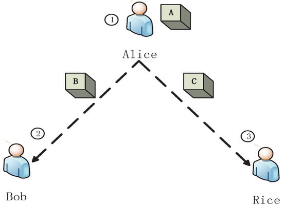
Figure 1.
A schematic tripartite dynamic zero-sum classical game . Alice puts a ball into three boxes , and . And then, she sends to Rice, and sends to Bob. Rice can choose to open or let Alice open . If Rice opens and there is no ball in it, it is Bob’s turn to open or ask Alice to open .
In the present games, we assume that the actions of different participants have a sequence, where the latter participant can observe the former’s action. There are four stages in the present model as follows.
- S1.
- Alice randomly puts a ball into one of three black boxes, , and . Alice sends the box to Rice, and sends to Bob.
- S2.
- Bob gives his own choice, i.e., he chooses to open or asks Alice to open , but he does not take any action.
- S3.
- Rice chooses her own strategy and takes action, i.e., she opens or lets Alice open . If Rice opens and there is no ball in the box, the game enters the fourth stage.
- S4.
- It is Bob’s turn to take action according the strategy he has chosen in S2, i.e., he opens box or asks Alice to open box .
Moreover, for any strategy combination, we assume that the total payment of all participants is zero. In the following, we will explore this kind of games with two settings with different gains.
The classical game tree is shown in Figure 2. In the stages of , the wining rules of the game are given by
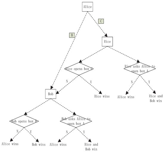
Figure 2.
The classical game tree. The rectangle with color represents the black box with the ball while the rectangle without color represents an entity, i.e., Alice, Bob and Rice. The diamond represents an operation. N means no ball being found, and Y means the ball being found.
- W1.
- Bob and Rice win if Rice chooses to open and finds the ball in S3.
- W2.
- Alice wins if Rice does not find the ball in box in S3.
- W3.
- Rice wins if Rice opens and finds the ball in S3.
- W4.
- Bob and Rice win if Bob opens and finds the ball in S4.
- W5.
- Alice wins if Bob opens and does not find the ball in in S4.
- W6.
- Bob wins if Bob opens box and finds the ball in S4.
- W7.
- Alice wins if Bob opens box and does not find the ball in S4.
Now, for convenience, we define the following probabilities.
- P1.
- Denote as the probability that Alice puts the ball into .
- P2.
- Denote as the probability that Alice puts the ball into or .
- P3.
- Denote as the probability that Rice chooses to open .
- P4.
- Denote as the probability that Bob chooses to open .
Here, we assume that Alice has equal probability to put the ball into or . It follows that , with .
From winning rules W1–W7 of , it is easy to get the winning probability for Rice from W3 (i.e., Rice finds the ball after opening ) is given by
Moreover, the winning probability for Bob from W6 (i.e., Rice chooses to open and does not find the ball, but Bob finds the ball after opening ) is given by
For Alice, there are three subcases W2, W5 and W7 for winning. It follows that
The winning probability for Bob from W1 and W4 is given by
The same result holds for Rice from W1 and W4, i.e., .
Here, we analyze players’ strategies for the present game to show the main idea. For Alice, she does not know which box Rice or Bob would choose to open before she prepares. Alice may lose the game if she puts the ball in one of the three boxes with a higher probability. Thus, there is a tradeoff for Alice to choose her strategy (the probability ). For Bob, he does not know which box Rice would to open when he gives the probability . So, he should consider a known parameter given by Alice and an unknown parameter given by Rice. Similar analysis can be applied to Rice’s strategy, Rice needs to choose her own parameter based on what she knows before she takes action.
2.2. The First Tripartite Classical Game
It is well known that every player will maximize its own interests in a non-cooperative game. In this section, we present the first game with the gain setting given in Table 1. Our goal is to show the no-fairness of this game with classical resources.

Table 1.
The gain settings of players in the first classical game . Here, denotes the gain of Rice (or Bob, or Alice). means that Rice finds the ball after opening box . means that Bob finds the ball after opening box . means that neither Rice or Bob finds the ball. means that either Rice or Bob successes by opening box . in the first classical game.
2.2.1. The Average Gain of Rice
From Table 1, the average gain of Rice is given by
From Equation (6), we get that the partial derivative of with respect to is given by
From Equation (6), if , is a deceasing function. In this case, Rice has to set to maximize her gains. If , i.e., is increasing function, Rice will choose to maximize her gains. Moreover, when , i.e., is a constant, can be any probability.
2.2.2. The Average Gain of Bob
Similar to Equation (6), we get that the average gain of Bob is given by
There are several cases to maximize . We only present one case in the following for explaining the main idea. The other cases are included in Appendix A.
For , i.e., , we get that . From Equation (8), we obtain
- C1.
- If , we get that . In this case, Bob chooses such that , where .
- C2.
- If , i.e., . Owing to , we get that can be any probability.
All the results are given in Table 2.
Table 2.
The values of and . depends on the different cases in the game, where . Here, denotes the intervals given by , , and .
2.2.3. The Average Gain of Alice
In this subsection, we calculate the average gain of Alice, which is denoted by . It is easy to write the expression for according to Table 1 as follows.
For the case of , it follows from Table 2 that and . Equation (9) is then rewritten into
where . It is easy to prove that achieves the maximum when . Denote , where is a small constant satisfying . It follows from Equation (10) that
By using the same method for the rest of cases (see Appendix B for details), we can get Table 3. From Table 3, we get that for , and for . Thus, Alice will choose to maximize her gain when , while when .
Table 3.
denotes the maximum of , and denotes the corresponding point of .
2.2.4. Fair Zero-Sum Game
From Section 2.2.3, we get that for . By using induction we know that and from Table 2. From Equations (6), (8) and (9), the expressions of , and with respect to are shown in Table 4.
Table 4.
The average gains of players in the first classical game .
Result 1 The tripartite game is unfair for any .
Proof.
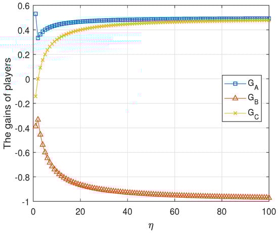
The numeric evaluations of , and are shown in Figure 3 for and . It shows that the tripartite classical game is unfair. Formally, since the tripartite game is a zero-sum game, i.e., the summation of the average gains of all players is zero. It is sufficient to prove that the gain of one player is strictly greater than that of the other. The proof is completed by two cases.
Figure 3.
The average gains of three parties in the first classical game . In this simulation, we assume and . The gain of Alice is strictly larger than the gains of Bob and Rice for any .
if is very small. This completes the proof. □
2.3. The Second Tripartite Classical Game
In this section, we present the second game with different settings shown in Table 5. The first game and the second game are the same except for the gain table, i.e., both games adopt the game model in Section 2.1. Similar to the first game , our goal is to prove its unfair.
Table 5.
The gain settings of the second game . Here, denotes gain of Rice (or Bob, or Alice). We assume that in this second game.
Similar to Section 2.2, we can evaluate the gains of all parties, as shown in Table 6. The details are shown in Appendix C, Appendix D and Appendix E. From Table 6, we can prove the following theorem.
Table 6.
The average gains of players in the second classical tripartite game .
Result 2 The tripartite classical game is unfair for any .
Proof.
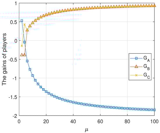
The numeric evaluations of , and are shown in Figure 4 for . It shows that the tripartite classical game is unfair. This can be proved formally as follows. From the assumption, the second classical game is zero-sum. It is sufficient to prove that there is no such that , and equal to zero. The proof is completed by two cases.
Figure 4.
The average gains of three parties in the second classical game . Here, . and and have no common intersection. Moreover, when , and coincide, but do not intersect with .
This completes the proof. □
3. Zero-Sum Quantum Games
In this section, by quantizing the classical game shown in Figure 1, we get that there are also four stages in quantum game, as shown in Figure 5. The correspondence between the classical and quantum game are: the classical game is to put a ball into three ordinary black boxes, while the quantum game is to put a particle into three quantum boxes. In the classical games, Bob and Rice can selectively let Alice open the box to prevent Alice from putting the ball into the box so that Bob and Rice cannot find the ball. In quantum game, they can prevent this same problem by setting the committed state before the game, i.e., Alice, Bob and Rice agree on which state Alice should set the photon to. Alice has three quantum boxes, , and used to store a photon. The state of the photon in the boxes are denoted , and . The quantum game is given by the following four stages S1–S4.
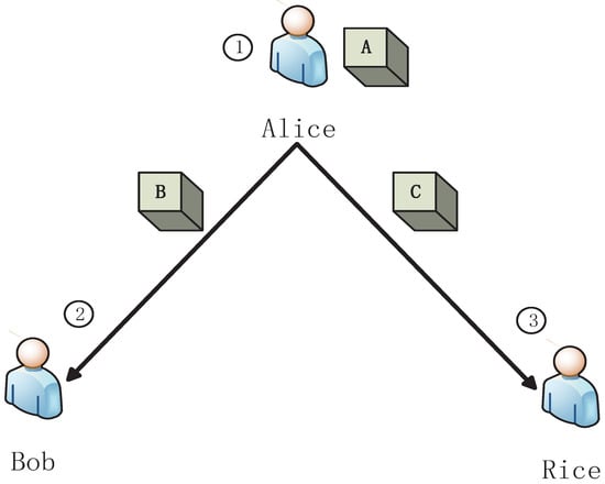
Figure 5.
The schematic model of tripartite dynamic zero-sum quantum game. Here, three parties use a single photon to complete the game while the classic game uses a ball in the game given in Figure 1.
- S1.
- Alice randomly puts the single photon into one of the three quantum boxes, , and . Alice sends the box to Rice, and sends to Bob.
- S2.
- Bob gives his own strategy, and he opens box .
- S3.
- Rice chooses her own strategy and takes action, i.e., she opens . If neither Rice nor Bob finds the photon, the game enters the fourth stage.
- S4.
- Bob(Rice) asks Alice to send him(her) box to verify whether the state of photon prepared by Alice is the same as the committed state.
Moreover, for any strategy combination, we assume that the total payment of all participants is zero and the latter participant can observe the former’s action. In the following, we will explore this kind of games with two settings with different gains.
The quantum game tree is shown in Figure 6. In the stages of , the wining rules of the game is given by
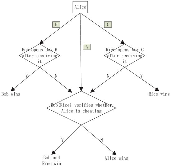
Figure 6.
The quantum game tree. The rectangle with color represents the black box with the photon while the rectangle without color represents an entity Alice. The diamond represents an operation. N means no photon being found, and Y means the photon being found.
- W1.
- Rice wins if Rice finds the photon after opening .
- W2.
- Bob wins if Bob finds the photon after opening .
- W3.
- Bob and Rice win if neither Rice nor Bob finds the photon but Alice is not honest.
- W4.
- Alice wins if neither Rice nor Bob finds the photon and Alice is honest.
We consider the dynamic zero-sum quantum game with the same setting parameters given in Table 1 and Table 5, but the difference is that each symbol has a slightly different meaning, i.e., in quantum games, means that Rice finds the photon after opening the box . means that Bob finds the photon after opening the box . means that neither Rice nor Bob finds the photon and Alice is honest. means that neither Rice nor Bob finds the photon but Alice is not honest.
3.1. The Winning Rules of The Quantum Game
The winning rules of quantum game is similar to W1–W4. For convenience we define the following probabilities.
- P1.
- Denote as the probability that Alice puts the photon into the box .
- P2.
- Denote as the probability that Alice puts the photon into box or box .
- P3.
- Denote as the probability that Rice chooses to open the box when she received .
- P4.
- Denote as the probability that Bob chooses to open the box when he received .
Similar to classical game shown in Figure 1, we have and .
In quantum scenarios, the box of , , or is realized by a quantum state or . The statement of one party finding the photon by opening one box ( for example) means that one party find the photon in the state after projection measurement under the basis . With these assumption, we get an experimental quantum game as follows.
Alice’s preparation. Alice prepares the single photon in the following supposition state
where and can be realized by using different paths, and is a parameter controlled by Alice.
Bob’s operation. Bob splits the box into box and box according the following transformation
where is a parameter controlled by Bob.
Rice’s operation. Rice splits the box into two parts and according to the following transformation
where is a parameter controlled by Rice.
Similar to classical games, Alice may choose a large to increase the probability of the photon appearing in box , which will then reduce the probability of Bob and Rice finding the photon. However, this strategy may result in losing the game with a high probability for Alice in the verification stage. Similar intuitive analysis holds for others. Hence, it should be important to find reasonable parameters for them. We give the detailed process in the following.
Suppose that Alice prepares the photon in the following state
using path encoding. When Bob (Rice) receives its box () and splits it into two parts, the final state of the photon is given by
From Equation (20), the probability that Rice finds the photon in (using single photon detector) is
Moreover, the probability that Bob finds the photon in is given by
If neither Rice nor Bob finds the photon, the state in Equation (20) will collapse into
If Alice did prepare the photon in the committed state initially, it is easy to prove that the state at this stage should be
where . By performing a projection measurement on , Rice or Bob gets an ideal state with the probability
where .
The probability that neither Rice nor Bob finds the photon when Alice did prepare the photon in the committed state is give by
Moreover, the probability that neither Rice nor Bob finds the photon but Rice or Bob detects forge state prepared by Alice is denote by or , which is given by
with from winning rule W3.
3.2. The First Tripartite Quantum Game
In this subsection, we introduce the quantum implementation of the first game with the gain setting shown in Table 1. Here, each symbol in Table 1 has a slightly different meaning, i.e., in quantum game, means that Rice finds the photon after opening the box . means that Bob finds the photon after opening the box . means that neither Rice or Bob finds the photon and Alice is honest. means that neither Rice or Bob finds the photon but Alice is not honest.
3.2.1. The Average Gain of Rice
Denote as Rice’s average gain. We can easily get according to Table 1 as follows
where .
The partial derivative of with respect to the variable is given by
Each participant has the perfect knowledge before the game reaching this stage, i.e., each participant is exactly aware of what previous participant has done. Hence, . Let . We get
If Alice chooses , the probability that Alice finds the photon will decrease while the probability that Rice or Bob detects the difference between the prepared and the committed states will increase in the verification stage. This means that Alice has no benefit if she chooses . It follows that and . Hence, from Equation (30) we get
From Equation (31), we get and . From Equations (30) and (31), is a decreasing function in x when and increasing when . Moreover, when , is a decreasing function in x. Since , gets the maximum value at for , or gets the maximum value at for , or gets the maximum value at for .
3.2.2. The Average Gain of Bob
Denote as the average gain of Bob. From Table 1, we get as
where .
The partial derivative of with respect to is given by
Similar to Equations (30) and (31), we can get
from .
From Equation (34), we obtain and . From Equations (33) and (34), decreases with and increases with . Moreover, decreases with . Since , gets the maximum value at for for , or gets the maximum value at for , or gets the maximum value at for . From , we get .
Similarly, we can get the detailed analysis of Rice, shown in Appendix F. The values of and which depend on in the first quantum game such that achieves the maximum are given in Table 7.
3.2.3. The Average Gain of Alice
Denote as the average gain of Alice. From Table 1, it is easy to evaluate as follows
where .
From Table 7, we discuss Alice’s gain in five cases. Here, we only discuss one of them. Other cases are shown in Appendix G.
If , i.e., , we get that
Denote
It follows that . In this case, we get . From Equation (36), we get that the average gain of Alice is given by
Note that from Equation (37). increases with when . So, gets the maximum value at , which is denoted by given by
where the corresponding point is denoted by .
By using the same method for other cases (see Appendix G), we get Table 8.
Table 8.
denotes the maximum of where the corresponding point is denoted by .
3.2.4. Quantum Fair Game
In this subsection, we prove the proposed quantum game is fair. From Equations (29) and (32) and Table 8 we get that
If ,,, from Table 8 we obtain that , and from Table 7. The average gains of three players are evaluated using and , as shown in Figure 7. Here, for each , the gains of Alice, Bob and Rice can tend to zero by changing .
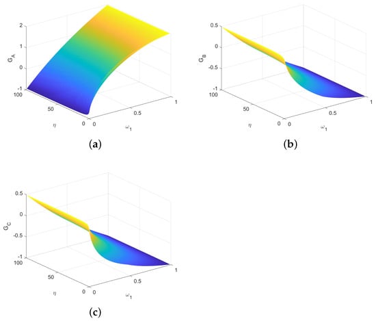
Figure 7.
The average gains of three parties depending on and . (a) The average gain of Alice. (b) The average gain of Bob. (c) The average gain of Rice.
From Figure 8a,b, we get that the degree of deviation from the fair game is very small even if the game is not completely fair. The game converges to the fair game when . To sum up, we get the following theorem.
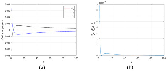
Figure 8.
(a) The average gains of Alice, Bob and Rice depending on . For each , the value of is equal to the value that minimizes the deviation of the game from fair game. (b) Degree of deviation. Here, we express the degree of deviation from the fair game as the sum of the squares of each player’s average gain.
Result 3 The first quantum game is asymptotically fair.
Proof.
Note that the first quantum game is zero-sum, i.e., the summation of the average gains of all players is zero. From Equation (36), Alice will make when , i.e., , in order to maximize her own gain, while Bob and Rice will choose accordingly. Hence, we get three gains as follows
Combining with the assumption of , we get from . Thus, when , the quantum game converges a fair game, i.e., asymptotically fair. This completes the proof. □
3.3. The Second Tripartite Quantum Game
In this section, we give the quantum realization of the second game . According to Table 5, similar to the first quantum game, the gain of Rice is given by
where . The detailed maximizing is shown in Appendix H.
Similarly, the gain of Bob is given by
Its maximization is shown in Appendix I.
The gain of Alice is given by
Its maximization is shown in Appendix J.
The numeric evaluations of average gains are shown in Figure 9 in terms of and . For each , we can make the gains of Alice, Bob and Rice equal to zero as much as possible by adjusting . The deviation degree is shown in Figure 10a. The relationship between the appropriate and is shown in Figure 10b. From Figure 10a,b, the degree of deviation from the fair game is very small even if the game is not completely fair. The game converges to the fair game when . To sum up, we get the following result.
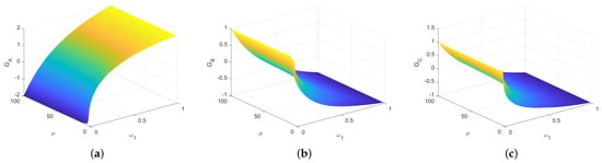
Figure 9.
The average gains of three parties depending on and .
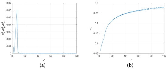
Figure 10.
(a) For each , the degree to which the game deviates from the fair game. Here, we express the degree of deviation from the game as the sum of the squares of each player’s average gain. (b) The relationship between the appropriate and .
Result 4 The second quantum game is asymptotically fair.
Proof.
Note that the second quantum game is zero-sum, i.e., the summation of the average gains of all players is zero. From Equation (46), Alice will make when , i.e., , in order to maximize her own gain, while Bob and Rice will choose accordingly. Hence, we get three gains as follows
We get and from . Thus, when , the quantum game converges a fair game, i.e., asymptotically fair. This completes the proof. □
4. Quantum Game with Noises
In this section, we consider quantum games with noises. One is from the experimental measurement. The other is from the preparation noise of resource state.
4.1. Experimental Measurement Error
In the case of measurement error, from Equation (20), we can get that the probability of Rice opens box and finds the photon becomes
where is measurement error which may be very small.
From Equation (20), we get the probability that Bob opens box and finds the photon is given by
Rice or Bob makes a projection measurement on for the verification the final state with success probability
where .
is the probability that neither Rice nor Bob finds the photon and Alice did prepare the photon in the committed state, is given by
where are given by
Since and , and is very small, denotes , which can be treated as measurement error. Thus Equation (49) can be rewritten as
The probability that neither Rice nor Bob finds the photon but Rice or Bob detects the forage preparation of Alice is denoted by or which given by
where from the winning rule W4.
4.2. White Noises
In this subsection, we consider that Alice prepares a noisy photon in the state
where denotes the identity operator, is given in Equation (16), and . After Bob’s and Rice’s splitting operation, the state of the photon becomes
where is given by
Denote as the probability that Rice finds the photon after opening the box . From Equation (53) it is given by
Denote as the probability that Bob finds the photon after opening the box . From Equation (53) it is given by
For the case that neither Bob nor Rice detects the photon, the density operator for the photon is given by
Now, Rice or Bob makes a projection measurement with positive operator on the photon for verifying the committed state of Alice with success probability
Denote as the probability that neither Rice nor Bob finds the photon, and Alice did prepare the photon in the committed state. It is easy to obtain that
Denote or as the probability that neither Rice nor Bob finds the photon but Rice or Bob detects the forage preparation. We obtain that
where from the winning rule W4.
Take the first quantum game as an example. The Rice’s average gain is given by
The partial derivative of with respect to is
where .
Assume that v is very close to one, i.e., . It follows that is bounded. Thus Equation (62) can be rewritten as
Similarly, we get
The partial derivative of with respect to is given by
where .
5. Conclusions
It has shown that two present quantum games are asymptotically fair. Interestingly, these games can be easily changed to biased versions from Figure 5 and Figure 8, by choosing different and . These kind of schemes may be applicable in gambling theory. Similar to bipartite scheme [27], a proof-of-principle optical demonstration may be followed for each scheme.
In this paper, we present one tripartite zero-sum game with different settings. This game is unfair if all parties use of classical resources. Interestingly, this can be resolved by using only pure state in similar quantum games. Comparing with the classical games, the present quantum games provide asymptotically fair. Moreover, these quantum games are robust against the measurement errors and preparation noises. This kind of protocols provide interesting features of pure state in resolving specific tasks. The present examples may be extended for multipartite games in theory. Unfortunately, these extensions should be nontrivial because of high complexity depending on lots of free parameters.
Author Contributions
Methodology, Writing—original draft, Writing—review and editing, H.-M.C. and M.-X.L. Both authors have read and agreed to the published version of the manuscript.
Funding
This work is supported by the National Natural Science Foundation of China (No.61772437) and Sichuan Youth Science and Technique Foundation (No.2017JQ0048).
Institutional Review Board Statement
Not applicable.
Informed Consent Statement
Not applicable.
Data Availability Statement
The data from numeric evaluations can be obtained from authors under proper requirements and goals.
Conflicts of Interest
The authors declare no conflict of interest.
Appendix A. The Average Gain of Bob in the First Classical Game
In order to calculate Bob’s average gain, we need to consider whether is greater than zero or not. And the case of has given in Section 2.2.2 The case of is as follows.
For , we have . In this case, . From Equation (8) we get
The partial derivative of with respect to is given by
Two cases will be considered as follows.
- (i)
- If , we get . In this case, there are two subcases.
- C1
- For , we get , and increases with . So, Bob should make in order to maximize his gains. From Equation (A1), we obtain
- C2
- For , we get . Hence, decreases with . Thus, Bob will let in order to maximize his gains. From Equation (A1), we get
- (ii)
- If , we get . Since , it follows that . Note that . It implies that increases with . Bob will set to maximize his gains. From Equation (A1), we obtain that
It is no doubt for Bob to choose the strategy which has higher gains. There are two options for Bob.
Case 1..
In this case, we get from Equations (8) and (A3) that
Suppose that . We get . The solution of this equation is given by and . It means that for and , and for . Note that
Moreover, it is easy to prove that
Similarly, we can get
From Equation (A9), we get for , and for .
To sum up we get the following result
- For , i.e., , we getfor
- For , i.e., , we getwhere .
Case 2..
In this case, from Equations (8) and (A4) we get
Thus for , where .
Appendix B. The Average Gain of Alice in the First Classical Game
For the case of , we have given in Section 2.2.3. The remaining three cases are as follows.
Case 1. For and , we have and . From Equation (9), we get
So, takes the maximum value at , which is then denoted by given by
Case 2. For and , we have and . From Equation (9), we get
The partial derivative of with respect to is given by
By setting , we get
Let . From Equation (A15), we get
The general solution of this equation is given by
By substituting , and into , we obtain that
Equation (A17) is a cubic equation about . It is the most likely to have three roots, i.e., , , with . So, decreases with for and . increases with for and . From Figure A1, we get . So, takes the maximum value at , which is then denoted by given by
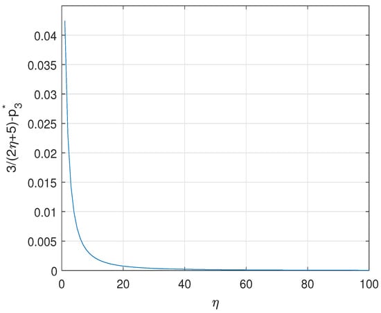
Figure A1.
The values of depending on .
Case 3. For , we have . From Equation (9), we get
From Equation (A20) decreases . Hence, the maximum value of is given by
Note that . Thus, gets the maximum value at for .
Appendix C. The Average Gain of RICE in the Second Classical Game
It is straightforward to calculate the average gain of Rice according to Table 5 as follows
The partial derivative of with respect to is given by
If , i.e., increases with , Rice will choose to maximize her gains. However, if , i.e., decreases with , Rice will set in order to maximize her gains.
Appendix D. The Average Gain of Bob in Classical Second Game
Similar to , we can get Bob’s average gain as follows
According to the sign of , we can divide it into two cases.
Case 1., i.e., .
In this case, . From Equation (A25) we get
The partial derivative of with respect to is given by
Here, we discuss it in three subcases.
- (i)
- For , we get . For , it follows that . It means that , i.e., decreases with . Thus, Bob will set to maximize his gains. From Equation (A24), we get
- (ii)
- For , we can get , and when , we get , i.e., increases with . So, Bob makes in order to maximize his gains. From Equation (A24), we can get that
- (iii)
- For , i.e., , when , we can get , i.e., decreases with . Thus, Bob will make to maximize his gains. From Equation (A24), we obtain that
Case 2., i.e., . For , we get .
In this case, we have and , where . From Equation (A24), we obtain that
If , we have . Bob will make to get the maximal gains for , where .
Table A1.
The values of and . The values of depend on the different cases in the game.
Table A1.
The values of and . The values of depend on the different cases in the game.
| Cases | |||
|---|---|---|---|
| 1 | 0 | ||
| 1 | 1 | 0 |
Appendix E. The Average Gain of Alice in the Second Classical Game
According to Table 5, we can get the average gain of Alice.
Here, three cases will be considered as follows.
Case 1. For , we get and . From Equation (A31), we get
which implies that
From , we have , i.e., increases with . It follows that . We obtain that the maximum value of as
Case 2. For , we get and . From Equation (A31), we get
The partial derivative of with respect to is given by
From Equation (A36), increases with for , and decreases for , thus the following three cases need to be considered according to it.
- (i)
- For , i.e., , decreases with . So, and . From Equation (A35), we get
- (ii)
- For , i.e., , increases with . So, and . From Equation (A35), we get
- (iii)
- For , i.e., , increases with for , and decreases for . So, takes its maximum at the point of . From Equation (A35), we get
Case 3. For , we have and , where . From Equation (A31), we get
It is easy to prove that decreases with . So, the maximum of achieves at , which is given by
It is easy to prove that for , and for , and for .
To sum up we get Table A2.
Table A2.
The maximum of and the corresponding point .
Table A2.
The maximum of and the corresponding point .
| Cases | ||
|---|---|---|
Appendix F. Analysis of β and γ in the First Quantum Game
How Rice and Bob choose their own parameters to maximize their average gains? we will discuss them in five cases.
Case 1. For , Rice should take to maximize her gains. Since , i.e., , Bob should take to maximize his gains. Hence, we have .
Case 2. For , Rice should take to maximize her gains. Since , i.e., , Bob should take to maximize his gains. Therefore, we get .
Case 3. For , if Bob takes , after knowing Bob’s actions, Rice will definitely choose to maximize her gains, i.e., . For Bob, when , decreases with . Hence, we have and . If Bob takes , after knowing Bob’s actions, Rice will definitely choose to maximize her gains. However, when , decreases with . In this case, we get and .
Case 4. For , if Bob takes , after knowing Bob’s actions, Rice will definitely choose to maximize her gains, i.e., . The reason is that decreases with for . From Bob’s own gains, it should be and . If Bob takes , Rice will definitely choose to maximize her gains after knowing Bob’s actions, i.e., , because decreases with for . In this case, from Bob’s own interests, we have and . Note that is decreasing function in for . So, we get and .
Case 5. For , if Bob takes , Rice will choose to maximize her gains after knowing Bob’s actions, i.e., . It is because Bob gets the maximum value at . We have and . If Bob takes , Rice will choose as close as possible to to maximize her gains after knowing Bob’s actions, i.e., . Thus, we obtain and .
Appendix G. The Average Gain of Alice in the First Quantum Game
We can calculate Alice’s average gain according to the values of and , and the first case of has been discussed in Section 3.2.3, the remaining four cases are as follows.
Case 1. For , i.e., , we get
Let , i.e., . In this case, we have . From Equation (36) we get
The derivative of with respect to is given by
The second derivative of with respect to is given by
From Equation (A45), we know that , and has at most one zero when . From , it follows that
Denote . If , i.e., , the solution of Equation (A46) is given by . is increasing function for , while it is decreasing for . From , achieves the maximum value at . If , i.e., , the solution of Equation (A46) is given by . is increasing function for , and decreasing for . From , gets the maximum value at . It means that gets the maximum value as
For , where the corresponding point is denoted by .
Case 2. For , i.e., , we get
where . In this case, we have and . From Equation (36) we have
From , we have . Equation (A49) is rewritten into
The derivative of with respect to is given by
The second derivative of with respect to is given by
From Equation (A52), we obtain that , and has at most one solution when . By letting , we get
Denote
The solution of Equation (A53) is given by . is increasing function when , or decreasing for . Thus, gets the maximum value at if , or gets the maximum value at if . Moreover, gets the maximum value at if . The maximum gain of Alice is denoted by when , where the corresponding point is denoted by .
Case 3. For , i.e., and , we get
where . In this case, we have and . From Equation (36) we get
The derivative of with respect to is given by
The second derivative of with respect to is given by
From Equation (A58), we know that , and has at most one zero when . By letting , we get
Let . If , the solution of Equation (A59) is given by . is increasing function for , while it is decreasing for . Thus, gets the maximum value at if , or at if . Moreover, gets the maximum value at if . The maximum gain of Alice gets is denoted by when , where the corresponding point is denoted by .
Case 4. For , i.e., , we get
where . In this case, we have and . From Equation (36) we get
The derivative of with respect to is given by
The second derivative of with respect to is given by
From Equation (A63), we have that , and has at most one zero when . By setting , we get
Let . The solution of Equation (A64) is given by . is increasing for , and decreasing for . is increasing for , and decreasing for . Thus, gets the maximum value at if , or at if . Moreover, gets the maximum value at if . The maximum gain of Alice is denoted by when , where the corresponding point is denoted by .
Appendix H. The Average Gain of Rice in the Second Quantum Game
According to Table A2, we get
where . The partial derivative of with respect to is given by
By setting , we get its solutions as
From Equation (A67), we know that and . From Equations (A66) and (A67), is decreasing for or , and increasing for . When, is decreasing in x. Since , when , achieves its maximum at . When , gets its maximum at . When , gets the maximum at .
Appendix I. The Average Gain of Bob in the Second Quantum Game
According to Table A2, we get that
The partial derivative of with respect to is given by
By setting , we get two solutions as
It follows that . Equation (A70) is then written into
From Equation (A71), we obtain and . From Equations (A69) and (A71), decreases with or , and increases for . Since , achieves its maximum at when . gets its maximum at when . When , gets the maximum at . From , we obtain .
Now, we make a brief analysis of the strategy of Rice and Bob as follows.
Case 1. For , both Rice and Bob should take to maximize its own gain from , i.e., . It follows that .
Case 2. For , both Rice and Bob should take to maximize the gain from , i.e., . Therefore, we have .
Case 3. For , we have for any being chosen by Bob. Rice will choose to maximize her gain. For Bob, increases with when , and decreases with when , So, we have and .
Case 4. For and , we have for any being chosen by Bob. Rice will choose to maximize her gain, i.e., . From Equation (A68), we get that
Case 5. For and , we have for any being chosen by Bob. Rice will choose to maximize her gain from . decreases with . It implies and . From Equation (A68), we get that
Thus if , we get that and . Otherwise, and .
Case 6. For and , we get that for any being chosen by Bob. Rice will choose to maximize her gain. For Bob, increases with when . So, and .
Case 7. For and , we have for any being chosen by Bob. Rice will choose to maximize her gain. We get that and . From Equation (A68), it implies that
Case 8. For and , we obtain that for any being chosen by Bob. Rice will choose to maximize her gain because of . decreases with . In this case, we get that and . From Equation (A68), we obtain that
Hence, if , we obtain that and . Otherwise, and .
Case 9. For , Rice will choose to maximize her gain if Bob chooses , i.e., . So, and . If Bob chooses , Rice will choose to maximize her gain. Note that decreases with when . It follows that and . Thus, and .
To sum up, we obtain that
Appendix J. The Average Gain of Alice in the Second Quantum Game
According to Table A2, we have
where .
The value of varies with the different values of and , we can calculate Alice’s average gain in the following nine cases according to that.
Case 1. For , it follows that . We get
where . In this case, . From Equation (A76), we obtain
From , we get that increases with when . So, gets the maximum at , which is denoted by given by
where the corresponding point is denoted by .
Case 2. For , it follows that . We get
where . In this case, . From Equation (A76) we get that
The derivative of with respect to is given by
The second derivative of with respect to is given by
From Equation (A83), we have , and has at most one solution when . By setting , we get
Denote . If , i.e., , the solution of Equation (A84) is given by . increases with when , and decreases with when . From , gets the maximum at . If , i.e., , the solution of Equation (A84) is given by . increases when , and decreases when . From , gets the maximum at . It means that gets the maximum when , which is further given by
where the corresponding point is denoted by .
Case 3. For , it follows that and . We get that
where
In this case, we get and . From Equation (A76), it follows that
The derivative of with respect to is given by
The second derivative of with respect to is given by
From Equation (A90), we know that , which implies that has at most one solution when . From , we get
Denote . The solution of Equation (A91) is given by . increases with , and decreases with . Thus, gets the maximum at if . If , gets the maximum at . If , gets the maximum at . The maximum gain of Alice when is denoted by , where the corresponding point is denoted by .
Case 4. For , i.e., and , we get
If , and , the maximum of Alice’s gain achieves when . The maximum is denoted by , where the corresponding point is denoted by .
Case 5. For and , and , the maximum of achieves when . The maximum is denoted by , where the corresponding point is denoted by .
Case 6. For and , i.e., and , we get
In this case, and . From Equation (A76), we get
The derivative of with respect to is given by
The second derivative of with respect to is given by
By setting , we get
Denote . The solution of Equation (A97) is given by . increases with , and decreases with . Thus, if , gets the maximum at . If , gets the maximum at . If , gets the maximum at . The maximum of achieves when and , and is then denoted by , where the corresponding point is denoted by .
Case 7. For , i.e., and , we get
where and . If , and , the maximum of achieves when , and is then denoted by , where the corresponding point is denoted by .
Case 8. For and , and , the maximum of achieves when , and is then denoted by , where the corresponding point is denoted by .
Case 9. For , i.e., , we get
In this case, and . From Equation (A76), we get
The derivative of with respect to is given by
The second derivative of with respect to is given by
From Equation (A102), we gave which implies that has at most one solution when . From , we get
Denote . The solution of Equation (A103) is given by . increases with , and decreases with . Thus, if , gets the maximum at . If , gets the maximum at . If , gets the maximum at . The maximum value of achievers when , and is then denoted by , where the corresponding point is denoted by .
References
- Streltsov, A.; Adesso, G.; Plenio, M.B. Colloquium: Quantum coherence as a resource. Rev. Mod. Phys. 2017, 89, 041003. [Google Scholar] [CrossRef]
- Bell, J.S. On the Einstein Podolsky Rosen paradox. Physics 1964, 1, 195. [Google Scholar] [CrossRef]
- Clauser, J.F.; Horne, M.A.; Shimony, A.; Holt, R.A. Proposed experiment to test local hidden-variable theories. Phys. Rev. Lett. 1969, 23, 880–884. [Google Scholar] [CrossRef]
- Landsburg, S.E. Quantum Game Theory. Not. Am. Math. Soc. 2004, 51, 394–399. [Google Scholar]
- Benjamin, S.C.; Hayden, P.M. Multi-player quantum games. Phys. Rev. A 2001, 64, 030301. [Google Scholar] [CrossRef]
- Flitney, A.P.; Schlosshauer, M.; Schmid, C.; Laskowski, W.; Hollenberg, L.C.L. Equivalence between Bell inequalities and quantum minority games. Phys. Lett. A 2008, 373, 521–524. [Google Scholar] [CrossRef]
- Murta, G.; Ramanathan, R.; Moller, N.; Cunha, M.T. Quantum bounds on multiplayer linear games and device-independent witness of genuine tripartite entanglement. Phys. Rev. A 2016, 93, 022305. [Google Scholar] [CrossRef]
- Luo, M.X. A nonlocal game for witnessing quantum networks. NPJ Quantum Inf. 2019, 5, 91. [Google Scholar] [CrossRef]
- Cleve, R.; Hoyer, P.; Toner, B.; Watrous, J. Consequences and limits of nonlocal strategies. In Proceedings of the 19th IEEE Conference on Computational Complexity (CCC2004), Amherst, MA, USA, 21–24 June 2004; pp. 236–249. [Google Scholar]
- Junge, M.; Palazuelos, C. Large violation of Bell inequalities with low entanglement. Commun. Math. Phys. 2011, 11, 1–52. [Google Scholar] [CrossRef]
- Briët, J.; Vidick, T. Explicit lower and upper bounds on the entangled value of multiplayer XOR games. Commun. Math. Phys. 2013, 321, 181–207. [Google Scholar] [CrossRef]
- Regev, O.; Vidick, T. Quantum XOR games. ACM Trans. Comput. Theory 2015, 7, 1–43. [Google Scholar] [CrossRef]
- Kempe, J.; Regev, O.; Toner, B. Unique games with entangled provers are easy. SIAM J. Comput. 2010, 39, 3207–3229. [Google Scholar] [CrossRef]
- Dinur, I.; Steurer, D.; Vidick, T. A parallel repetition theorem for entangled projection games. Comput. Complex. 2013, 24, 201–254. [Google Scholar] [CrossRef]
- Yuen, H. A Parallel Repetition Theorem for All Entangled Games. In Proceedings of the 43rd International Colloquium on Automata, Languages, and Programming (ICALP 2016), Rome, Italy, 11–15 July 2016; Volume 77. [Google Scholar]
- Jain, R.; Pereszlenyi, A.; Yao, P. A parallel repetition theorem for entangled two-player one-round games under product distributions. In Proceedings of the CCC’14, 2014 IEEE 29th Conference on Computational Complexity, Vancouver, BC, Canada, 11–13 June 2014; pp. 209–216. [Google Scholar]
- Brakerski, Z.; Kalai, Y.T. A Parallel Repetition Theorem for Leakage Resilience. In TCC’12, Proceedings of the 9th International Conference on Theory of Cryptography, Taormina, Sicily, Italy, 19–21 March 2012; Springer: Berlin, Germany, 2012; pp. 248–265. [Google Scholar]
- Ekert, A.K. Quantum cryptography based on Bell’s theorem. Phys. Rev. Lett. 1991, 67, 661. [Google Scholar] [CrossRef] [PubMed]
- Lim, C.C.W.; Portmann, C.; Tomamichel, M.; Renner, R.; Gisin, N. Device-Independent Quantum Key Distribution with Local Bell Test. Phys. Rev. X 2013, 3, 031006. [Google Scholar] [CrossRef]
- Vazirani, U.; Vidick, T. Fully device-independent quantum key distribution. Phys. Rev. Lett. 2014, 113, 140501. [Google Scholar] [CrossRef]
- Werner, R.F. Optimal cloning of pure states. Phys. Rev. A 1998, 58, 1827. [Google Scholar] [CrossRef]
- Marinatto, L.; Weber, T. A quantum approach to static games of complete information. Phys. Lett. A 2000, 272, 291–303. [Google Scholar] [CrossRef]
- Eisert, J.; Wilkens, M.; Lewenstein, M. Quantum games and quantum strategies. Phys. Rev. Lett. 1999, 83, 3077. [Google Scholar] [CrossRef]
- Sekiguchi, Y.; Sakahara, K.; Sato, T. Uniqueness of Nash equilibria in a quantum Cournot duopoly game. J. Phys. A Math. Theor. 2010, 43, 145303. [Google Scholar] [CrossRef]
- Brassard, G.; Broadbent, A.; Tapp, A. Recasting Mermin’s multi-player game into the framework of pseudo-telepathy. Quantum Inf. Comput. 2005, 5, 538–550. [Google Scholar]
- Meyer, D.A. Quantum strategies. Phys. Rev. Lett. 2012, 82, 1052. [Google Scholar] [CrossRef]
- Zhang, P.; Zhou, X.-Q.; Wang, Y.-L.; Shadbolt, P.J.; Zhang, Y.-S.; Gao, H.; Li, F.-L.; O’Brien, J.L. Quantum gambling based on Nash equilibrium. NPJ Quantum Inf. 2017, 3, 24. [Google Scholar] [CrossRef]
- Almeida, M.L.; Bancal, J.D.; Brunner, N.; Acin, A.; Gisin, N.; Pironio, S. Guess your neighbors input: A multipartite nonlocal game with no quantum advantage. Phys. Rev. Lett. 2010, 104, 230404. [Google Scholar] [CrossRef]
- Fudenberg, D.; Tirole, J. Game Theory; MIT Press: London, UK, 1995. [Google Scholar]
- Daskalakis, C.; Goldberg, P.W.; Papadimitriou, C.H. The complexity of computing a Nash equilibrium. Commun. ACM 2009, 52, 89–97. [Google Scholar] [CrossRef]


Publisher’s Note: MDPI stays neutral with regard to jurisdictional claims in published maps and institutional affiliations. |
© 2021 by the authors. Licensee MDPI, Basel, Switzerland. This article is an open access article distributed under the terms and conditions of the Creative Commons Attribution (CC BY) license (http://creativecommons.org/licenses/by/4.0/).