Optimal Noise Enhanced Signal Detection in a Unified Framework

Abstract

In this paper, a new framework for variable detectors is formulated in order to solve different noise enhanced signal detection optimal problems, where six different disjoint sets of detector and discrete vector pairs are defined according to the two inequality-constraints on detection and false-alarm probabilities. Then theorems and algorithms constructed based on the new framework are presented to search the optimal noise enhanced solutions to maximize the relative improvements of the detection and the false-alarm probabilities, respectively. Further, the optimal noise enhanced solution of the maximum overall improvement is obtained based on the new framework and the relationship among the three maximums is presented. In addition, the sufficient conditions for improvability or non-improvability under the two certain constraints are given. Finally, numerous examples are presented to illustrate the theoretical results and the proofs of the main theorems are given in the Appendix.

1. Introduction

Noise commonly exists with the useful signal, and more noises in the system often lead to less channel capacity and worse detectability. People usually try to utilize a series of filters and algorithms to remove the unnecessary noise. Hence, understanding and mastering the distribution and characteristics of noise is an essential research topic in traditional signal detection theory. Nevertheless, although it may seem very counterintuitive, noise does play an active role in many signal processing problems, and the performance of some nonlinear systems can be enhanced via adding noise under certain conditions [1,2,3,4,5,6,7,8,9,10,11,12,13,14,15,16,17,18,19,20,21,22,23,24,25,26,27]. The phenomenon that noise benefits system is the so-called stochastic resonance (SR), which was first proposed by Benzi et al. [1] in 1981 when they studied the periodic recurrence of ice gases. The positive effects of noise have drawn the attention of researchers in various fields. For example, the effect of SR on the global stability of complex networks is investigated in [26]. Kohar and Sinha demonstrated how to utilize noise to make a bistable system behave as a memory device in [27].

In the signal detection problem, researchers commonly care about how to increase the output signal-to-noise (SNR) [7,8,9,10,11], the mutual information [12,13], or detection probability with a constant false alarm rate [14,15,16,17,18,19,20], or how to decrease the Bayes risk [21,22] or the probability of error [23] by adding additive noise to the input of system or changing the background noise level. As presented in [8], the output SNR obtained by adding suitable noise to the input of system is higher than the input SNR. The research results in [14] indicate that the detection probability of the sign detector can be increased by adding an appropriate amount of white Gaussian noise.

Depending on the detection metrics, the SR phenomenon for the hypothesis testing or detection problems are usually investigated according to the Bayesian, Minimax or Neyman–Pearson criteria. In [23], the additive noise to optimize the performance of a suboptimal detector is explored according to Bayesian criterion under uniform cost assignment. It is demonstrated that the optimal noise to minimize the probability of error is a constant, and the improvability obtained by adding the constant noise can also be achieved via shifting the decision region without adding any additive noise. The probability distribution of the optimal additive noise to minimize Bayes risk is investigated in [21] according to the restricted Bayesian criterion, which can be extended to Bayesian and Minimax criteria easily. For an M-ary hypothesis testing problem, the optimal noise is determined as a randomization of at most M mass points.

In [15], a mathematical framework is established to search the optimal noise to maximize the detection probability based on Neyman–Pearson criterion. This leads to the very significant conclusion that the optimal noise is determined as the randomization of at most two discrete vectors. In addition, sufficient conditions whether the detection probability can or cannot be increased are given. However, from the perspective of Patel [18], the proof of the optimal noise presented in [15] has a little bit of a drawback. Moreover, the same noise enhanced problem for a fixed detector is researched through establishing a different mathematical framework in [18], where the optimal noise to maximize detection probability is also proved as a random signal consisting of no more than two discrete points and the corresponding probabilities. The researchers in [16] studied the noise enhanced detection performance for variable detectors according to the Neyman–Pearson criterion based on the results in [15]. The optimal noise enhanced solution to maximize the detection probability is determined as a randomization of no more than two detector and constant vector pairs.

Through the comparison and analysis above, it is clear that most researchers have focused on the maximization of detection probability via additive noise and there are few studies which cover the field of the minimization of the false-alarm probability. We cannot exclude the possibility that the false-alarm probability can be decreased by adding noise without deteriorating the original detectability, especially for the case where the detection probability cannot be increased via adding any noise. For example, a noise enhanced model which can increase the detection probability and decrease the false-alarm probability simultaneously by adding noise is first formulated in [25] for a fixed detector. In addition, the model is solved by a convex combination of the optimal noises for two limited cases, i.e., the minimization of false-alarm probability and the maximization of detection probability. Nevertheless, it is obvious that the convex combination is usually not the optimal solution of the maximum overall improvement of the model. In this paper, we explore the optimal solution to maximize the overall improvement of detection and false-alarm probabilities directly instead of the convex combination. In practical applications, though the structure of the detector commonly cannot be replaced in many cases, some parameters of the detector can be varied to obtain a better performance. Moreover, the noise enhanced detection problems for a fixed detector can generally be achieved by simplifying the results for variable detectors directly. Thus, it is necessary to discuss the noise enhanced detection problems on the premise of variable detectors.

In order to obtain the optimal noise enhanced solution to maximize the overall improvement of detection and false-alarm probabilities for variable detectors under two inequality-constraints, we formulate a new framework to define six different disjoint sets of detector and discrete vector pairs based on the signs of the relative improvements of the detection and the false-alarm probabilities. Then we explore the optimal noise enhanced solutions for the maximum detection probability and the minimum false-alarm probability and give the corresponding algorithms in the new framework. Further, through some derivation, the optimal noise enhanced solution for the maximum overall improvement of detection and false-alarm probabilities is proved as a randomization of at most two detector and discrete vector pairs from two different sets, and the relationship among the three maximums is presented. In addition, the theoretical results for the case of allowing the randomization between detectors can be applied straightforwardly to the case where the randomization between detectors cannot be allowed. Namely, the optimization problem for variable detectors is simplified to choose a fixed detector and search the optimal additive noise when the randomization between detectors cannot be allowed. Actually, the maximization of detection probability in this paper is equivalent to the noise enhanced detection problem for variable detectors studied in [16], which also needs all information of detection and false-alarm probabilities obtained by every detector and discrete vector pair. Indeed, the new framework subdivides the one set in [16] into six subintervals. Based on the definition of the six sets, it is obvious that each detector and discrete vector pair as a component of additive noise is available, partially available, or unavailable to meet the two constraints. Then the available and partial available pairs can be utilized to construct the optimal noise enhanced solutions to satisfy different requirements. Namely, the division of six sets effectively provides the foundation for maximizing the relative improvements of detection and false-alarm probabilities, and the sum of them.

The main contributions of this paper can be summarized as follows:

• Formulation of a new framework, where six different disjoint sets of detector and discrete vector pairs are defined according to two inequality-constraints.
• Algorithms for the noise enhanced solutions to maximize the relative improvements of the detection and the false-alarm probabilities are given based on the new framework.
• Noise enhanced solution of the maximum overall improvability is first provided based on the new framework and the relationship among the three maximums is explored.
• Determination of the sufficient conditions for the improvability and nonimprovability under the two constraints.

The remainder of this paper is organized as follows: in Section 2, three optimization problems for a binary hypothesis testing problem for a variable detector are proposed and the six disjoint sets of detector and discrete vector pairs are defined. In Section 3, the optimal noise enhanced solutions for the three optimization problem are discussed when the randomization between detectors can or cannot be allowed and the corresponding algorithms are given. Numerical results are presented in Section 4 and the conclusions are provided in Section 5.

2. Problem Formulation

Consider a binary hypothesis testing problem as follows:

$$H_i:p_i(\mathbf{x}), i=0,1$$

(1)

where $p_i(\mathbf{x})$ is the probability density function (pdf) of the observation $\mathbf{x}$ under $H_i$, $i=0,1$, and $\mathbf{x}\in {\text{ℝ}}^K$. For any $\mathbf{x}$, the probability of choosing $H_1$ can be characterized by $\varphi (\mathbf{x})$ and $0\le \varphi (\mathbf{x})\le 1$. Generally, $\varphi (\mathbf{x})$ is also treated as a decision function of the detector. In order to investigate the possible enhancement of detectability, a new noise modified observation $\mathbf{y}$ is obtained by adding an independent noise $\mathbf{v}$ to the original observation $\mathbf{x}$, i.e., $\mathbf{y}=\mathbf{x}+\mathbf{v}$. Correspondingly, the pdf of $\mathbf{y}$ under $H_i$ can be expressed by the convolutions of $p_i(\mathbf{x})$ and $p_{\mathbf{v}}(\mathbf{x})$ as below:

$$p_{\mathbf{y}}(\mathbf{y};H_i)=p_i(\mathbf{x})\ast p_{\mathbf{v}}(\mathbf{x})={\displaystyle {\int }_{{\text{ℝ}}^K}{p}_i(\mathbf{y}-\mathbf{v})p_{\mathbf{v}}(\mathbf{v})}d\mathbf{v}$$

(2)

where $\ast$ represents the symbol of convolution.

For the same detector, the decision function for $\mathbf{y}$ is the same as that for $\mathbf{x}$. Then the detection and false-alarm probabilities based on the new noise modified observation $\mathbf{y}$ are calculated by:

$$P_D^y={\displaystyle {\int }_{R^K}\varphi (\mathbf{y})p_{\mathbf{y}}(\mathbf{y};H_1)d\mathbf{y}}$$

(3)

$$P_{FA}^y={\displaystyle {\int }_{R^K}\varphi (\mathbf{y})p_{\mathbf{y}}(\mathbf{y};H_0)d\mathbf{y}}$$

(4)

According to the two constraints that $P_D^y\ge \beta$ and $P_{FA}^y\le \alpha$, where $\beta$ and $\alpha$ represent the lower limit on the detection probability and the upper limit on the false-alarm probability, respectively, the following three important definitions are given by:

$$z^d=P_D^y-\beta$$

(5)

$$z^{fa}=\alpha -P_{FA}^y$$

(6)

$$z=z^d+z^{fa}$$

(7)

where $z^d$ and $z^{fa}$ can be regarded as the relative improvements of the detection and false-alarm probabilities obtained by adding additive noise, respectively, and $z$ is the sum of $z^d$ and $z^{fa}$.

In many cases, though the structure of the detector cannot be substituted, some parameters of it can be varied, such as decision threshold. In addition, the whole detector can also be replaced in some special cases. Instead of a fixed decision function $\varphi (\cdot )$, we suppose that there exist a set of candidate decision functions written as $\Phi$ and any $\varphi \in \Phi$ can be utilized. Then for any decision function ${\varphi }_{\ell }\in \Phi$, $\ell =1,\dots ,L$, the detection and false-alarm probabilities based on $\mathbf{y}$ can be obtained by replacing $\varphi$ with ${\varphi }_{\ell }$, i.e.:

$$P_{D,{\varphi }_{\ell }}^y={\displaystyle {\int }_{R^K}{\varphi }_{\ell }(\mathbf{y})p_{\mathbf{y}}(\mathbf{y};H_1)d\mathbf{y}}$$

(8)

$$P_{FA,{\varphi }_{\ell }}^y={\displaystyle {\int }_{R^K}{\varphi }_{\ell }(\mathbf{y})p_{\mathbf{y}}(\mathbf{y};H_0)d\mathbf{y}}$$

(9)

When the additive noise is a discrete vector with pdf $\delta (\mathbf{v}-\mathit{v})$, where $\delta$ denotes the delta function, i.e., $\delta (\mathbf{v}-\mathit{v})=1$ only if $\mathbf{v}=\mathit{v}$ and $\delta (\mathbf{v}-\mathit{v})=0$ otherwise, $p_{\mathbf{y}}(\mathbf{y};H_i)=p_i(\mathbf{y}-\mathit{v})$. The corresponding noise modified detection and false-alarm probabilities can be rewritten as:

$$P_{D,{\varphi }_{\ell }}^y(\mathit{v})={\displaystyle {\int }_{R^K}{\varphi }_{\ell }(\mathbf{y})p_1(\mathbf{y}-\mathit{v})d\mathbf{y}}$$

(10)

$$P_{FA,{\varphi }_{\ell }}^y(\mathit{v})={\displaystyle {\int }_{R^K}{\varphi }_{\ell }(\mathbf{y})p_0(\mathbf{y}-\mathit{v})d\mathbf{y}}$$

(11)

Accordingly, under the constraints of $P_D^y\ge \beta$ and $P_{FA}^y\le \alpha$, the relative improvements of the detection and false-alarm probabilities corresponding to the additive noise with pdf $\delta (\mathbf{v}-\mathit{v})$ can be written as:

$$z_{{\varphi }_{\ell }}^d(\mathit{v})=P_{D,{\varphi }_{\ell }}^y(\mathit{v})-\beta$$

(12)

$$z_{{\varphi }_{\ell }}^{fa}(\mathit{v})=\alpha -P_{FA,{\varphi }_{\ell }}^y(\mathit{v})$$

(13)

Correspondingly:

$$z_{{\varphi }_{\ell }}(\mathit{v})=z_{{\varphi }_{\ell }}^d(\mathit{v})+z_{{\varphi }_{\ell }}^{fa}(\mathit{v})$$

(14)

In order to make full use of the information gained by the discrete vector $\mathit{v}$, we define the following six mutually disjoint sets for each ${\varphi }_{\ell }\in \Phi$ according to the values of $z_{{\varphi }_{\ell }}^d(\mathit{v})$ and $z_{{\varphi }_{\ell }}^{fa}(\mathit{v})$ denoted by $M_{1,{\varphi }_{\ell }}=\{({\varphi }_{\ell },\mathit{v})|z_{{\varphi }_{\ell }}^d(\mathit{v})>0,z_{{\varphi }_{\ell }}^{fa}(\mathit{v})>0\}$, $M_{2,{\varphi }_{\ell }}=\{({\varphi }_{\ell },\mathit{v})|z_{{\varphi }_{\ell }}^d(\mathit{v})>0,z_{{\varphi }_{\ell }}^{fa}(\mathit{v})=0\}$, $M_{3,{\varphi }_{\ell }}=\{({\varphi }_{\ell },\mathit{v})|z_{{\varphi }_{\ell }}^d(\mathit{v})=0,z_{{\varphi }_{\ell }}^{fa}(\mathit{v})>0\}$, $M_{4,{\varphi }_{\ell }}=\{({\varphi }_{\ell },\mathit{v})|z_{{\varphi }_{\ell }}^d(\mathit{v})>0,z_{{\varphi }_{\ell }}^{fa}(\mathit{v})<0\}$, $M_{5,{\varphi }_{\ell }}=\{({\varphi }_{\ell },\mathit{v})|z_{{\varphi }_{\ell }}^d(\mathit{v})<0,z_{{\varphi }_{\ell }}^{fa}(\mathit{v})>0\}$, $M_{6,{\varphi }_{\ell }}=\{({\varphi }_{\ell },\mathit{v})|z_{{\varphi }_{\ell }}^d(\mathit{v})\le 0,z_{{\varphi }_{\ell }}^{fa}(\mathit{v})\le 0\}$. Further, define $M_{{\varphi }_{\ell }}=\underset{j=1}{\overset{6}{\cup }}{M}_{j,{\varphi }_{\ell }}$ and $M_j=\underset{\ell =1}{\overset{L}{\cup }}{M}_{j,{\varphi }_{\ell }}$, then $M=\underset{\ell =1}{\overset{L}{\cup }}{M}_{{\varphi }_{\ell }}=\underset{j=1}{\overset{6}{\cup }}{M}_j$, where $j=1,\dots ,6$ and $\ell =1,\dots ,L$.

Accordingly, a framework is formulated by defining the six different sets. As a result, the purpose of this paper is to investigate the optimal noise enhanced solutions for the maximum $z^d$, $z^{fa}$ and $z$, respectively, under the two inequality-constraints based on the new framework. Obviously, whether the pair of $(\varphi ,\mathit{v})$ is useful, partially useful or unuseful for the noise enhancement can be determined according to the definitions of the six sets. For instance, any detector and discrete pair of $M_1$, $M_2$ and $M_3$ can meet the two constraints that $P_D^y\ge \beta$ and $P_{FA}^y\le \alpha$, the maximum $z^d$ may be obtained by a suitable detector and discrete pair of $M_1$ or $M_2$, the maximum $z^{fa}$ may be achieved by a detector and discrete pair of $M_1$ or $M_3$, and the maximum $z$ may be reached by a suitable detector and discrete pair of $M_1$, $M_2$ or $M_3$. In the following sections, the corresponding theorems and algorithms are provided.

3. The Noise Enhanced Solutions

Let $z_m^d$, $z_m^{fa}$ and $z_m$ be the maximum achievable $z^d$, $z^{fa}$ and $z$, respectively, which are obtained by adding a discrete vector as additive noise when the randomization between detectors is allowed. Namely, $z_m^d=\underset{(\varphi ,\mathit{v})\in M}{\max }{z}_{\varphi }^d(\mathit{v})$, $z_m^{fa}=\underset{(\varphi ,\mathit{v})\in M}{\max }{z}_{\varphi }^{fa}(\mathit{v})$ and $z_m=\underset{(\varphi ,\mathit{v})\in M}{\max }{z}_{\varphi }(\mathit{v})$. If anyone of $z_m^d$, $z_m^{fa}$ and $z_m$ is less than zero, $P_D^y\ge \beta$ and $P_{FA}^y\le \alpha$ cannot be obtained by adding any noise. So this paper is studied under the conditions that $z_m^d$, $z_m^{fa}$ and $z_m$ are greater than zero.

In general, when the randomization between different detectors is allowed, the noise enhanced solution can be viewed as a randomization of one or more detector and noise pairs with the corresponding weights. Suppose that the additive noise pdf is for any ${\varphi }_{\ell }\in \Phi$, $\ell =1,\dots ,L$, then $z^d$, $z^{fa}$ and $z$ can be expressed as:

$$z^d={\displaystyle \sum _{\ell =1}^L{\lambda }_{\ell }}{\displaystyle {\int }_{{\text{ℝ}}^K}{P}_{D,{\varphi }_{\ell }}^y(\mathit{v})p_{\mathbf{v},{\varphi }_{\ell }}(\mathit{v})d\mathit{v}}-\beta ={\displaystyle \sum _{\ell =1}^L{\lambda }_{\ell }}{\displaystyle {\int }_{{\text{ℝ}}^K}{z}_{{\varphi }_{\ell }}^d(\mathit{v})p_{\mathbf{v},{\varphi }_{\ell }}(\mathit{v})d\mathit{v}}$$

(15)

$$z^{fa}=\alpha -{\displaystyle \sum _{\ell =1}^L{\lambda }_{\ell }}{\displaystyle {\int }_{{\text{ℝ}}^K}{P}_{FA,{\varphi }_{\ell }}^y(\mathit{v})p_{\mathbf{v},{\varphi }_{\ell }}(\mathit{v})d\mathit{v}}={\displaystyle \sum _{\ell =1}^L{\lambda }_{\ell }}{\displaystyle {\int }_{{\text{ℝ}}^K}{z}_{{\varphi }_{\ell }}^{fa}(\mathit{v})p_{\mathbf{v},{\varphi }_{\ell }}(\mathit{v})d\mathit{v}}$$

(16)

$$z=z^d+z^{fa}={\displaystyle {\int }_{{\text{ℝ}}^K}[z_{{\varphi }_{\ell }}^d(\mathit{v})+z_{{\varphi }_{\ell }}^{fa}(\mathit{v})]p_{\mathbf{v},{\varphi }_{\ell }}(\mathit{v})d\mathit{v}}={\displaystyle \sum _{\ell =1}^L{\lambda }_{\ell }}{\displaystyle {\int }_{{\text{ℝ}}^K}{z}_{{\varphi }_{\ell }}(\mathit{v})p_{\mathbf{v},{\varphi }_{\ell }}(\mathit{v})d\mathit{v}}$$

(17)

where $0\le {\lambda }_{\ell }\le 1$ and ${\displaystyle \sum _{\ell =1}^L{\lambda }_{\ell }}=1$. Generally, the additive noise for any ${\varphi }_{\ell }\in \Phi$ can be viewed as a randomization of finite or infinite discrete vectors, i.e., $p_{\mathbf{v},{\varphi }_{\ell }}(\mathit{v})={\displaystyle \sum _{\kappa =1}^N{\eta }_{\kappa ,{\varphi }_{\ell }}\delta (\mathit{v}-{\mathit{v}}_{\kappa ,{\varphi }_{\ell }})}$, where $0\le {\eta }_{\kappa ,{\varphi }_{\ell }}\le 1$ and ${\displaystyle \sum _{\kappa =1}^N{\eta }_{\kappa ,{\varphi }_{\ell }}}=1$, and $N$ is a finite or infinite positive integer.

3.1. The Optimal Noise Enhanced Solution to Maximize z^d

From Equation (15), $z^d$ can be rewritten as:

$$\begin{array}{ll}{z}^d& ={\displaystyle \sum _{\ell =1}^L{\lambda }_{\ell }}{\displaystyle {\int }_{{\text{ℝ}}^K}{z}_{{\varphi }_{\ell }}^d(\mathit{v}){\displaystyle \sum _{\kappa =1}^N{\eta }_{\kappa ,{\varphi }_{\ell }}\delta (\mathit{v}-{\mathit{v}}_{\kappa ,{\varphi }_{\ell }})}d\mathit{v}}\\ & ={\displaystyle \sum _{i=1}^L{\displaystyle \sum _{k=1}^N{\lambda }_{\ell }{\eta }_{\kappa ,{\varphi }_{\ell }}}}{\displaystyle {\int }_{{\text{ℝ}}^K}{z}_{{\varphi }_{\ell }}^d(\mathit{v})\delta (\mathit{v}-{\mathit{v}}_{\kappa ,{\varphi }_{\ell }})d\mathit{v}}\\ & ={\displaystyle \sum _{\ell =1}^L{\displaystyle \sum _{\kappa =1}^N{\lambda }_{\ell }{\eta }_{\kappa ,{\varphi }_{\ell }}}}{z}_{{\varphi }_{\ell }}^d({\mathit{v}}_{\kappa ,{\varphi }_{\ell }})\end{array}$$

(18)

Further, $z^d$ can also be expressed by:

$$z^d={\displaystyle \sum _{\tau =1}^6{\displaystyle \sum _{j=1}^6{\displaystyle \sum _{\kappa =1}^N{\tau }_{\tau j\kappa }[{\xi }_{\tau j\kappa }{z}_{{\varphi }_h}^d({\mathit{v}}_{\tau \kappa ,{\varphi }_h})+(1-{\xi }_{\tau j\kappa })z_{{\varphi }_l}^d({\mathit{v}}_{j\kappa ,{\varphi }_l})]}}}$$

(19)

where $({\varphi }_h,{\mathit{v}}_{\tau \kappa ,{\varphi }_h})\in M_{\tau }$, $({\varphi }_l,{\mathit{v}}_{j\kappa ,{\varphi }_l})\in M_j$, $\tau \ne j$, ${\displaystyle \sum _{\tau =1}^6{\displaystyle \sum _{j=1}^6{\displaystyle \sum _{\kappa =1}^N{\tau }_{\tau j\kappa }}}}=1$, $0\le {\tau }_{\tau j\kappa }\le 1$, $0\le {\xi }_{\tau j\kappa }\le 1$, $h,l=1,\dots ,L$. Let $z_{\tau j\kappa }^d={\xi }_{\tau j\kappa }{z}_{{\varphi }_h}^d({\mathit{v}}_{\tau \kappa ,{\varphi }_h})+(1-{\xi }_{\tau j\kappa })z_{{\varphi }_l}^d({\mathit{v}}_{j\kappa ,{\varphi }_l})$. In other words, $z_{\tau j\kappa }^d$ is obtained by the randomization of two detector and discrete vector pairs from two different sets, i.e., $({\varphi }_h,{\mathit{v}}_{\tau \kappa ,{\varphi }_h})\in M_{\tau }$ and $({\varphi }_l,{\mathit{v}}_{j\kappa ,{\varphi }_l})\in M_j$. Then $z^d={\displaystyle \sum _{\tau =1}^6{\displaystyle \sum _{j=1}^6{\displaystyle \sum _{\kappa =1}^N{\tau }_{\tau j\kappa }{z}_{\tau j\kappa }^d}}}$ is the convex combination of multiple $z_{\tau j\kappa }^d$, which means that $z^d$ can be obtained by the randomization of multiple different randomizations consisting of two detector and discrete vector pairs $({\varphi }_h,{\mathit{v}}_{{\varphi }_h})$, $({\varphi }_l,{\mathit{v}}_{{\varphi }_l})$ from two different sets with the corresponding probabilities. From Equation (18), if there exists at least one detector and discrete vector pair which belongs to $M_1$, the constraints $P_D^y\ge \beta$ and $P_{FA}^y\le \alpha$ can be satisfied by choosing the suitable detector and adding the discrete vector. Otherwise, according to Equation (19) and the definitions of $M_1~M_6$, a randomization of two detector and discrete vector pairs from two different sets may satisfy the two constraints $P_D^y\ge \beta$ and $P_{FA}^y\le \alpha$.

Let the maximum achievable $z^d$ obtained by any noise solution under the two constraints that $P_D^y\ge \beta$ and $P_{FA}^y\le \alpha$ be denoted by $z_{opt}^d$. Define $Q_d=\{(\varphi ,\mathit{v})|\mathit{v}=\arg \underset{(\varphi ,\mathit{v})\in M}{\max }{z}_{\varphi }^d(\mathit{v})\}$ be the set of all detector and discrete vector pairs corresponding to $z_m^d$. Then the following theorem and corollary hold and the corresponding proofs are presented in Appendix A.

Theorem 1. 

$z_{opt}^d$ can be achieved by the randomization of at most two detector and discrete vector pairs $({\varphi }_1,{\mathit{v}}_1)$ and $({\varphi }_2,{\mathit{v}}_2)$ from two different sets, i.e., $({\varphi }_1,{\mathit{v}}_1)\in M_{\tau }, ({\varphi }_2,{\mathit{v}}_2)\in M_j, \tau ,j=1,\dots ,6$ and $\tau \ne j$.

Corollary 1. 

(a) If there exists at least one pair $({\varphi }_o,{\mathit{v}}_o)$ of $Q_d$ which belongs to $M_1\cup M_2, z_{opt}^d$ can be obtained by selecting $({\varphi }_o,{\mathit{v}}_o)$ and $z_{opt}^d=z_m^d$. (b) When $Q_d\subset M_4$, the $z^{fa}$ corresponding to $z_{opt}^d$ is zero. (c) When $Q_d\subset M_4, z_{opt}^d$ is obtained by the randomization of $({\varphi }_1,{\mathit{v}}_1)\in M_4$ and $({\varphi }_2,{\mathit{v}}_2)$ from $M_1, M_3$ or $M_5$ with the respective probabilities $\xi =\frac{-z_{{\varphi }_2}^{fa}({\mathit{v}}_2)}{z_{{\varphi }_1}^{fa}({\mathit{v}}_1)-z_{{\varphi }_2}^{fa}({\mathit{v}}_2)}$ and $1-\xi$, or the detector and discrete pair $({\varphi }_o,{\mathit{v}}_o)=\arg \underset{(\varphi ,\mathit{v})\in M_2}{\max }{z}_{\varphi }^d(\mathit{v})$.

Next, we try to search the maximum achievable $z^d$ obtained by the randomization of $({\varphi }_1,{\mathit{v}}_1)\in M_4$ and $({\varphi }_2,{\mathit{v}}_2)$ from $M_1$, $M_3$ or $M_5$ when $Q_d\subset M_4$. Generally, the corresponding $z^d$ and $z^{fa}$ can be expressed by:

$$z^d=\xi z_{{\varphi }_1}^d({\mathit{v}}_1)+(1-\xi )z_{{\varphi }_2}^d({\mathit{v}}_2)={\displaystyle \sum _{i=1}^2{\xi }_i}{z}_{{\varphi }_i}^d({\mathit{v}}_i)$$

(20)

$$z^{fa}=\xi z_{{\varphi }_1}^{fa}({\mathit{v}}_1)+(1-\xi )z_{{\varphi }_2}^{fa}({\mathit{v}}_2)={\displaystyle \sum _{i=1}^2{\xi }_i}{z}_{{\varphi }_i}^{fa}({\mathit{v}}_i)$$

(21)

where ${\xi }_1=\xi$ and ${\xi }_2=1-\xi$. Under the constraint that $P_{FA}^y\le \alpha$, the Lagrangian of the optimization problem of maximizing $z^d$ can be formulated as:

$$L(p_{\varphi ,v},k)=z^d+k{z}^{fa}={\displaystyle \sum _{i=1}^2{\lambda }_i}[z_{{\varphi }_i}^d({\mathit{v}}_i)+k{z}_{{\varphi }_i}^{fa}({\mathit{v}}_i)]$$

(22)

where $p_{\varphi ,\mathit{v}}$ denotes the distribution of $({\varphi }_1,{\mathit{v}}_1)$ and $({\varphi }_2,{\mathit{v}}_2)$. According to the Lagrange duality, we have:

$$\underset{p_{\varphi ,\mathit{v}}}{\max }\hspace{0.17em}{z}^d=\underset{k\ge 0}{\min }\hspace{0.17em}\underset{p_{\varphi ,\mathit{v}}}{\max }L(p_{\varphi ,\mathit{v}},k)$$

(23)

So solving the optimal solution to maximize $z^d$ is equivalent to finding $k>0$ and $p_{\varphi ,\mathit{v}}$ to make Equation (23) hold. Let us define an auxiliary function $d_{\varphi }(\mathit{v},k)$ such that:

$$d_{\varphi }(\mathit{v},k)=z_{\varphi }^d(\mathit{v})+k\cdot z_{\varphi }^{fa}(\mathit{v})$$

(24)

Let $d_1(k)$ and $d_2(k)$ be the respective suprema of $d_{\varphi }(\mathit{v},k)$ over the sets $M_4$ and $M_1\cup M_3\cup M_5$, i.e.,

$$d_1(k)=\underset{(\varphi ,\mathit{v})}{\sup }\{d_{\varphi }(\mathit{v},k):(\varphi ,\mathit{v})\in M_4\}$$

(25)

$$d_2(k)=\underset{(\varphi ,\mathit{v})}{\sup }\{d_{\varphi }(\mathit{v},k):(\varphi ,\mathit{v})\in M_1\cup M_3\cup M_5\}$$

(26)

Due to $z_{\varphi }^{fa}(\mathit{v})<0$ when $(\varphi ,\mathit{v})\in M_4$, $d_1(k)$ is a decreasing function of $k$. When $(\varphi ,\mathit{v})\in M_1\cup M_3\cup M_5$, $z_{\varphi }^{fa}(\mathit{v})>0$, which means $d_2(k)$ increases with $k$. Thus, there exists one $k^{*}>0$ such that $d_1(k^{*})=d_2(k^{*})=d^{*}$, i.e., there are $({\varphi }_1,{\mathit{v}}_1)\in M_4$ and $({\varphi }_2,{\mathit{v}}_2)\in M_1\cup M_3\cup M_5$ such that $d_{{\varphi }_1}({\mathit{v}}_1,k^{*})=d_1(k^{*})=d_2(k^{*})=d_{{\varphi }_2}({\mathit{v}}_2,k^{*})=d^{*}$. So the $z^{fa}$ and the $z^d$ obtained by the randomization between $({\varphi }_1,{\mathit{v}}_1)$ and $({\varphi }_2,{\mathit{v}}_2)$ with the respective probabilities $\xi =\frac{-z_{{\varphi }_2}^{fa}({\mathit{v}}_2)}{z_{{\varphi }_1}^{fa}({\mathit{v}}_1)-z_{{\varphi }_2}^{fa}({\mathit{v}}_2)}$ and $1-\xi$ can be calculated by:

$$z^{fa}=\xi z_{{\varphi }_1}^{fa}({\mathit{v}}_1)+(1-\xi )z_{{\varphi }_2}^{fa}({\mathit{v}}_2)=\frac{-z_{{\varphi }_2}^{fa}({\mathit{v}}_2)}{z_{{\varphi }_1}^{fa}({\mathit{v}}_1)-z_{{\varphi }_2}^{fa}({\mathit{v}}_2)}{z}_{{\varphi }_1}^{fa}({\mathit{v}}_1)+\frac{z_{{\varphi }_1}^{fa}({\mathit{v}}_1)}{z_{{\varphi }_1}^{fa}({\mathit{v}}_1)-z_{{\varphi }_2}^{fa}({\mathit{v}}_2)}{z}_{{\varphi }_2}^{fa}({\mathit{v}}_2)=0$$

(27)

$$\begin{array}{ll}{z}^d& =\xi z_{{\varphi }_1}^d({\mathit{v}}_1)+(1-\xi )z_{{\varphi }_2}^d({\mathit{v}}_2)\\ & =\xi (d^{*}-k^{*}{z}_{{\varphi }_1}^{fa}({\mathit{v}}_1))+(1-\xi )(d^{*}-k^{*}{z}_{{\varphi }_2}^{fa}({\mathit{v}}_2))\\ & =d^{*}-k^{*}(\xi z_{{\varphi }_1}^{fa}({\mathit{v}}_1)+(1-\xi )z_{{\varphi }_2}^{fa}({\mathit{v}}_2))\\ & =d^{*}\end{array}$$

(28)

Combined with Equations (27) and (28), the $k^{*}$ and the randomization of $({\varphi }_1,{\mathit{v}}_1)$ and $({\varphi }_2,{\mathit{v}}_2)$ are the solution of Equation (23), i.e., $d^{*}$ is the maximum achievable $z^d$ obtained by the randomization of $({\varphi }_1,{\mathit{v}}_1)\in M_4$ and $({\varphi }_2,{\mathit{v}}_2)$ from $M_1$, $M_3$ or $M_5$ when $Q_d\subset M_4$. Based on the analysis above, Algorithm B1 is provided in Appendix B to search the two detector and discrete vector pairs.

3.2. The Optimal Noise Enhanced Solution to Maximize z^fa

In this subsection, the optimal noise enhanced solution to maximize $z^{fa}$ is considered. Let the maximum achievable $z^{fa}$ obtained by any noise solution under the two constraints that $P_D^y\ge \beta$ and $P_{FA}^y\le \alpha$ be denoted by $z_{opt}^{fa}$. Define $Q_{fa}=\{(\varphi ,\mathit{v})|\mathit{v}=\arg \underset{(\varphi ,\mathit{v})\in M}{\max }{z}_{\varphi }^{fa}(\mathit{v})\}$. Then the following theorem and corollary hold and the corresponding proofs are omitted here, which are similar to Theorem 1 and Corollary 1, respectively.

Theorem 2. 

$z_{opt}^{fa}$ can be obtained by the randomization of at most two detector and discrete vector pairs $({\varphi }_1,{\mathit{v}}_1)$ and $({\varphi }_2,{\mathit{v}}_2)$ from two different sets, i.e., $({\varphi }_1,{\mathit{v}}_1)\in M_{\tau }, ({\varphi }_2,v_2)\in M_j, \tau ,j=1,\dots ,6$ and $\tau \ne j$.

Corollary 2. 

(a) If there exists at least one pair $({\varphi }_o,{\mathit{v}}_o)$ of $Q_{fa}$ which also belongs to $M_1\cup M_3$, $z_{opt}^{fa}$ can be achieved by selecting $({\varphi }_o,{\mathit{v}}_o)$ and $z_{opt}^{fa}=z_m^{fa}$. (b) When $Q_{fa}\subset M_5$, the $z^d$ corresponding to $z_{opt}^{fa}$ is zero. (c) When $Q_{fa}\subset M_5$, $z_{opt}^{fa}$ is obtained by the randomization of $({\varphi }_1,{\mathit{v}}_1)$ from $M_1$, $M_2$ or $M_4$ and $({\varphi }_2,{\mathit{v}}_2)\in M_5$ with the respective probabilities $\eta =\frac{-z_{{\varphi }_2}^d({\mathit{v}}_2)}{z_{{\varphi }_1}^d({\mathit{v}}_1)-z_{{\varphi }_2}^d({\mathit{v}}_2)}$ and $1-\eta$, or the detector and discrete pair $({\varphi }_o,{\mathit{v}}_o)=\arg \underset{(\varphi ,v)\in M_3}{\max }{z}_{\varphi }^{fa}(\mathit{v})$.

Then we focus on the maximum $z^{fa}$ obtained by the randomization of $({\varphi }_1,{\mathit{v}}_1)$ from $M_1$, $M_2$ or $M_4$ and $({\varphi }_2,{\mathit{v}}_2)\in M_2$ with respective probabilities $\eta$ and $1-\eta$ when $Q_{fa}\subset M_5$. The corresponding $z^d$ and $z^{fa}$ can be expressed by:

$$z^d=\eta z_{{\varphi }_1}^d({\mathit{v}}_1)+(1-\eta )z_{{\varphi }_2}^d({\mathit{v}}_2)={\displaystyle \sum _{i=1}^2{\eta }_i}{z}_{{\varphi }_i}^d({\mathit{v}}_i)$$

(29)

$$z^{fa}=\eta z_{{\varphi }_1}^{fa}({\mathit{v}}_1)+(1-\eta )z_{{\varphi }_2}^{fa}({\mathit{v}}_2)={\displaystyle \sum _{i=1}^2{\eta }_i}{z}_{{\varphi }_i}^{fa}({\mathit{v}}_i)$$

(30)

where ${\eta }_1=\eta$ and ${\eta }_2=1-\eta$. Under the constraint of $P_D^y\ge \beta$, the Lagrangian of the maximization of $z^{fa}$ is:

$$L(p_{\varphi ,\mathit{v}},t)=z^{fa}+t{z}^d={\displaystyle \sum _{i=1}^2{\eta }_i}[z_{{\varphi }_i}^{fa}({\mathit{v}}_i)+t{z}_{{\varphi }_i}^d({\mathit{v}}_i)]$$

(31)

The Lagrange duality suggests that:

$$\underset{p_{\varphi ,\mathit{v}}}{\max }{z}^{fa}=\underset{k\ge 0}{\min }\hspace{0.17em}\underset{p_{\varphi ,\mathit{v}}}{\max }L(p_{\varphi ,\mathit{v}},t)$$

(32)

In order to solve Equation (32), let us define an auxiliary function $f_{\varphi }(\mathit{v},t)$ such that:

$$f_{\varphi }(\mathit{v},t)=z_{\varphi }^{fa}(\mathit{v})+t\cdot z_{\varphi }^d(\mathit{v})$$

(33)

Suppose that $f_1(t)$ and $f_2(t)$ are the respective suprema of $f_{\varphi }(\mathit{v},t)$ over the sets $M_1\cup M_2\cup M_4$ and $M_5$, i.e.,

$$f_1(t)=\underset{(\varphi ,\mathit{v})}{\sup }\{f_{\varphi }(\mathit{v},t):(\varphi ,\mathit{v})\in M_1\cup M_2\cup M_4\}$$

(34)

$$f_2(t)=\underset{(\varphi ,\mathit{v})}{\sup }\{f_{\varphi }(\mathit{v},t):(\varphi ,\mathit{v})\in M_5\}$$

(35)

When $(\varphi ,\mathit{v})\in M_1\cup M_2\cup M_4$, $z_{\varphi }^d(\mathit{v})>0$ and then $f_1(t)$ increases with $t$. Since $z_{\varphi }^d(\mathit{v})<0$ when $(\varphi ,\mathit{v})\in M_5$, $f_2(t)$ decreases with $t$. So there exists a $t^{*}>0$ such that $f_1(t^{*})=f_2(t^{*})=f^{*}$. Namely, there exist $({\varphi }_1,{\mathit{v}}_1)\in M_1\cup M_2\cup M_4$ and $({\varphi }_2,{\mathit{v}}_2)\in M_5$ such that $f_{{\varphi }_1}({\mathit{v}}_1,t^{*})=f_1(t^{*})=f_2(t^{*})=f_{{\varphi }_2}({\mathit{v}}_2,t^{*})=f^{*}$. The $z^d$ and the $z^{fa}$ obtained by the randomization between $({\varphi }_1,{\mathit{v}}_1)$ and $({\varphi }_2,{\mathit{v}}_2)$ with the respective probabilities $\eta =\frac{-z_{{\varphi }_2}^d({\mathit{v}}_2)}{z_{{\varphi }_1}^d({\mathit{v}}_1)-z_{{\varphi }_2}^d({\mathit{v}}_2)}$ and $1-\eta$ can be calculated by:

$$z^d=\eta z_{{\varphi }_1}^d({\mathit{v}}_1)+(1-\eta )z_{{\varphi }_2}^d({\mathit{v}}_2)=\frac{-z_{{\varphi }_2}^d({\mathit{v}}_2)}{z_{{\varphi }_1}^d({\mathit{v}}_1)-z_{{\varphi }_2}^d({\mathit{v}}_2)}{z}_{{\varphi }_1}^d({\mathit{v}}_1)+\frac{z_{{\varphi }_1}^d({\mathit{v}}_1)}{z_{{\varphi }_1}^d({\mathit{v}}_1)-z_{{\varphi }_2}^d({\mathit{v}}_2)}{z}_{{\varphi }_2}^d({\mathit{v}}_2)=0$$

(36)

$$\begin{array}{ll}{z}^{fa}& =\eta z_{{\varphi }_1}^{fa}({\mathit{v}}_1)+(1-\eta )z_{{\varphi }_2}^{fa}({\mathit{v}}_2)\\ & =\eta (f^{*}-t^{*}{z}_{{\varphi }_1}^d({\mathit{v}}_1))+(1-\eta )(f^{*}-t^{*}{z}_{{\varphi }_2}^d({\mathit{v}}_2))\\ & =f^{*}-t^{*}(\eta z_{{\varphi }_1}^d({\mathit{v}}_1)+(1-\eta )z_{{\varphi }_2}^d({\mathit{v}}_2))\\ & =f^{*}\end{array}$$

(37)

From Equations (36) and (37), the $t^{*}$ and the randomization of $({\varphi }_1,{\mathit{v}}_1)$ and $({\varphi }_2,{\mathit{v}}_2)$ are the solution of Equation (32), i.e., $f^{*}$ is the maximum achievable $z^{fa}$ obtained by the randomization of $({\varphi }_1,{\mathit{v}}_1)$ from $M_1$, $M_2$ or $M_4$ and $({\varphi }_2,{\mathit{v}}_2)\in M_5$ when $Q_{fa}\subset M_5$. According to the derivation above, Algorithm B2 presented in Appendix B can be utilized to search the corresponding detector and discrete vector pairs.

3.3. The Optimal Noise Enhanced Solution to Maximize z

Let $z_{opt}$ represent the maximum achievable $z$ under the two constraints that $P_D^y\ge \beta$ and $P_{FA}^y\le \alpha$. Define $Q_z=\{(\varphi ,\mathit{v})|\mathit{v}=\arg \underset{(\varphi ,\mathit{v})\in M}{\max }{z}_{\varphi }(\mathit{v})\}$. Next, the optimal noise enhanced solution to maximize $z$ is explored in this subsection, the related theorem and corollary are provided as below.

Theorem 3. 

$z_{opt}$ can be obtained by the randomization of at most two detector and discrete vector pairs $({\varphi }_1,{\mathit{v}}_1)$ and $({\varphi }_2,{\mathit{v}}_2)$ from two different sets such that $({\varphi }_1,{\mathit{v}}_1)\in M_{\tau }$, $({\varphi }_2,{\mathit{v}}_2)\in M_j$ and $\tau \ne j$. The proof of Theorem 3 is also similar to Theorem 1 and omitted here.

Corollary 3. 

(a) If there exists at least one pair $({\varphi }_o,{\mathit{v}}_o)$ of $Q_z$ belongs to $M_1\cup M_2\cup M_3$, the maximum $z$ can be realized by choosing $({\varphi }_o,{\mathit{v}}_o)$ and $z_{opt}=z_m$. (b) If $Q_z\subset M_4\cup M_5$, $z_{opt}=\max (z_{opt}^d,z_{opt}^{fa})$. (c) If $Q_z\cap M_4\ne \varnothing$ and $Q_z\cap M_5\ne \varnothing$, we have $z_{opt}^d=z_{opt}^{fa}=z_{opt}=z_m$. The proofs are provided in Appendix A.

Especially, when $Q_z\subset M_4\cup M_5$, we can select the two pairs $({\varphi }_1,{\mathit{v}}_1)$ and $({\varphi }_2,{\mathit{v}}_2)$ directly, according to the analysis above and the properties of $M_1~M_5$, to form an available noise enhanced solution to make the value of $z$ as greater as possible.

If $Q_z\subset M_4$, then we can let $({\varphi }_1,{\mathit{v}}_1)\in Q_z$ and $({\varphi }_2,{\mathit{v}}_2)\in M_1\cup M_3\cup M_5$. Since $z_{{\varphi }_1}({\mathit{v}}_1)\ge z_{{\varphi }_2}({\mathit{v}}_2)$, the maximum $z$ is achieved when $\lambda ={\lambda }_2=\frac{-z_{{\varphi }_2}^{fa}({\mathit{v}}_2)}{z_{{\varphi }_1}^{fa}({\mathit{v}}_1)-z_{{\varphi }_2}^{fa}({\mathit{v}}_2)}$. The greater the value of $\lambda$, the greater the value of $z$. So $({\varphi }_1,{\mathit{v}}_1)$ and $({\varphi }_2,{\mathit{v}}_2)$ can be selected as $({\varphi }_1,{\mathit{v}}_1)=\arg \underset{(\varphi ,\mathit{v})\in Q_z}{\max }{z}_{\varphi }^{fa}(\mathit{v})$ and $({\varphi }_2,{\mathit{v}}_2)=\arg \underset{(\varphi ,\mathit{v})\in T_1}{\max }{z}_{\varphi }^{fa}(\mathit{v})$, where $T_1=\{(\varphi ,\mathit{v})|(\varphi ,\mathit{v})=\arg \underset{(\varphi ,\mathit{v})\in M_1\cup M_3\cup M_5}{\max }{z}_{\varphi }(\mathit{v})\}$.

Similarly, when $Q_z\subset M_5$, let $({\varphi }_2,{\mathit{v}}_2)=\arg \underset{(\varphi ,\mathit{v})\in Q_z}{\min }{z}_{\varphi }^d(\mathit{v})$ and $({\varphi }_1,{\mathit{v}}_1)=\arg \underset{(\varphi ,\mathit{v})\in T_2}{\min }{z}_{\varphi }^d(\mathit{v})$, where $T_2=\{(\varphi ,\mathit{v})|(\varphi ,\mathit{v})=\arg \underset{(\varphi ,\mathit{v})\in M_1\cup M_2\cup M_4}{\max }{z}_{\varphi }(\mathit{v})\}$.

3.4. Sufficient Conditions for $P_D^y\ge \beta$ and $P_{FA}^y\le \alpha$

In this section, according to the analysis from Section 3.1 to Section 3.3 and the properties of the six sets, the sufficient conditions which can or cannot satisfy the two constraints $P_D^y\ge \beta$ and $P_{FA}^y\le \alpha$ are determined as below.

Theorem 4. 

(a) If $M_1\cup M_2\cup M_3\ne \varnothing$, any pair $(\varphi ,\mathit{v})\in M_1\cup M_2\cup M_3$ can meet $P_D^y\ge \beta$ and $P_{FA}^y\le \alpha$; (b) When $M_1\cup M_2\cup M_3=\varnothing$, if there exist $({\varphi }_1,{\mathit{v}}_1)\in M_4$ and $({\varphi }_2,{\mathit{v}}_2)\in M_5$ such that:

$$|z_{{\varphi }_1}^{fa}({\mathit{v}}_1)|\cdot |z_{{\varphi }_2}^d({\mathit{v}}_2)|<|z_{{\varphi }_1}^d({\mathit{v}}_1)|\cdot |z_{{\varphi }_2}^{fa}({\mathit{v}}_2)|$$

(38)

then $P_D^y\ge \beta$ and $P_{FA}^y\le \alpha$ can be realized by the randomization of $({\varphi }_1,{\mathit{v}}_1)$ and $({\varphi }_2,{\mathit{v}}_2)$, otherwise there exists no noise enhanced solution to make $P_D^y\ge \beta$ and $P_{FA}^y\le \alpha$hold. The proofs are presented in Appendix A.

When no randomization between detectors is allowed, only one detector can be selected to utilize. Suppose that the selected detector is ${\varphi }_o$, the conclusions for the case of allowing randomization between detectors can be applied to the case of nonrandomization between detectors straightforwardly by replacing $M_j$ with $M_{j,{\varphi }_o}$ and ${\varphi }_1={\varphi }_2={\varphi }_o$, where $j=1,\dots ,6$.

4. Numerical Results

In this section, a binary hypothesis-testing problem is considered to verify the theoretical results explored in the previous sections. The binary hypotheses are given by:

$$\{\begin{array}{l}{H}_0:x[i]=\omega [i]\\ H_1:x[i]=A+\omega [i]\end{array}$$

(39)

where $i=0,\dots ,K-1$, $A>0$ is a known constant, and $\omega [i]$ are independent identically distributed (i.i.d.) symmetric Gaussian mixture noise samples such that:

$$p_{\omega }(\omega )=\frac{1}{2}\gamma (\omega ;-\mu ,{\sigma }^2)+\frac{1}{2}\gamma (\omega ;\mu ,{\sigma }^2)$$

(40)

where $\gamma (\omega ;\mu ,{\sigma }^2)=(1/\sqrt{2\pi {\sigma }^2})\exp (-{(\omega -\mu )}^2/2{\sigma }^2)$. The test statistic of a suboptimal detector is shown as:

$$T(x)=\frac{1}{K}{\displaystyle \sum _{i=0}^{K-1}(\frac{1}{2}+\frac{1}{2}\mathrm{sgn}(x[i]))}=\frac{1}{K}{\displaystyle \sum _{i=0}^{K-1}(S(x[i]))}\genfrac{}{}{0ex}{}{\stackrel{H_1}{>}}{\underset{H_0}{<}}\gamma$$

(41)

where $S(t)=\frac{1}{2}+\frac{1}{2}\mathrm{sgn}(t)=\{\begin{array}{l}1,t>0\\ 0,t<0\end{array}$. From Equation (41), the test result in this case is obtained through twice decision. Firstly, use the sign detector $S(\cdot )$ to determine the sign of each observation component $x[i]$. Secondly, compute the proportion of the positive observation components in the observation vector and then compare it with the decision threshold $\gamma$ to obtain the final result.

Let $K=2$, then the detector shown in Equation (41) can be substituted by two decision thresholds $\gamma =1$ and $\gamma =0.5$, the corresponding decision function are ${\varphi }_1$ and ${\varphi }_2$, respectively. When $\gamma =1$, the detector chooses $H_1$ only if $x[0]>0$ and $x[1]>0$ at the same time. When $\gamma =0.5$, the detector chooses $H_1$ if $x[0]>0$ or $x[1]>0$. Assume $\mathit{v}={(v_1,v_2)}^T$ be a discrete vector without any constraints. Then the detection and false-alarm probabilities of the sign detector $S(\cdot )$ choosing the noise modified observation component $y[i]=x[i]+v[i]>0$, $i=0,1$, can be calculated by $P_{1,s}(v[i])={\displaystyle {\int }_{-\infty }^{\infty }S(y[i])p_1(y[i]-v[i])dy[i]}=\frac{1}{2}Q(\frac{-v[i]-\mu -A}{\sigma })+\frac{1}{2}Q(\frac{-v[i]+\mu -A}{\sigma })$ and $P_{0,s}(v[i])={\displaystyle {\int }_{-\infty }^{\infty }S(y[i])p_0(y[i]-v[i])dy[i]}=\frac{1}{2}Q(\frac{-v[i]-\mu }{\sigma })+\frac{1}{2}Q(\frac{-v[i]+\mu }{\sigma })$, where $v[0]=v_1$, $v[1]=v_2$ and $Q(x)={\displaystyle {\int }_x^{+\infty }(1/\sqrt{2\pi })}\exp (-t^2/2)dt$. Further, the detection and false-alarm probabilities of $y$ for ${\varphi }_1$ are computed as $P_{D,{\varphi }_1}^y(\mathit{v})=P_{1,s}(v_1)P_{1,s}(v_2)$ and $P_{FA,{\varphi }_1}^y(\mathit{v})=P_{0,s}(v_1)P_{0,s}(v_2)$, respectively. The detection and false-alarm probabilities of $y$ for ${\varphi }_2$ can be expressed by $P_{D,{\varphi }_2}^y(\mathit{v})=1-(1-P_{1,s}(v_1))(1-P_{1,s}(v_2))$ and $P_{FA,{\varphi }_2}^y(\mathit{v})=1-(1-P_{0,s}(v_1))(1-P_{0,s}(v_2))$. Correspondingly, $z_{{\varphi }_i}^d(\mathit{v})=P_{D,{\varphi }_i}^y(\mathit{v})-\beta$ and $z_{{\varphi }_i}^{fa}(\mathit{v})=\alpha -P_{FA,{\varphi }_i}^y$, $i=1,2$.

Let $\mu =3$ and $A=1$. Under the two constraints that $P_{FA}^y\le \alpha$ and $P_D^y\ge \beta$, for any $\sigma$, we can determine the six sets $M_{j,{\varphi }_i}$, $j=1,\dots ,6$, for ${\varphi }_1$ and ${\varphi }_2$ according to the definitions of the six sets and the values of $z_{{\varphi }_i}^d(\mathit{v})$ and $z_{{\varphi }_i}^{fa}(\mathit{v})$, respectively. Naturally, the six sets obtained by allowing the randomization between ${\varphi }_1$ and ${\varphi }_2$ can be determined by $M_j=M_{j,{\varphi }_1}\cup M_{j,{\varphi }_2}$, $j=1,\dots ,6$. Afterwards, we can search the maximum $z^d$, $z^{fa}$, $z$ and the corresponding noise enhanced solutions according to the algorithm provided in Section 3.

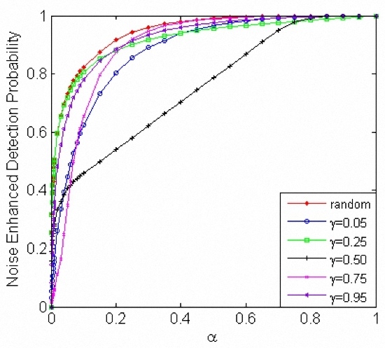
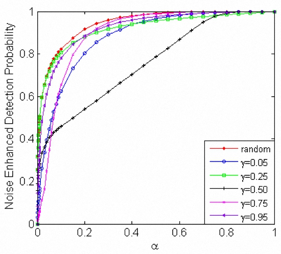
Figure 1 illustrates that the maximum achievable $z^d$, $z^{fa}$ and $z$ for ${\varphi }_1$, ${\varphi }_2$ and the case of allowing the randomization between ${\varphi }_1$ and ${\varphi }_2$ for different values of $\sigma$ when $\alpha =0.3$ and $\beta =0.7$. The $z^d$ plotted in Figure 1a is actually the relative improvement of the maximum achievable detection probability $P_{D,opt}^y$ compared to $\beta =0.7$ under the constraint $P_{FA}^y\le \alpha =0.3$, i.e., $z^d=P_{D,opt}^y-\beta$. Hence, $P_{FA}^y\le \alpha$ and $P_D^y\ge \beta$ can be realized only when $z^d\ge 0$. As shown in Figure 1a, $z^d<0$ when $\sigma$ increases to a certain extent, which means the feasible range of $\sigma$ for the noise enhanced phenomenon is limited. When $\sigma$ is close to 0, the maximum achievable $z^d$ for ${\varphi }_1$ is 0.3, which equals to that for the case of allowing the randomization between detectors, and the corresponding $P_{D,opt}^y$ is close to 1 while the maximum $P_D^y$ for ${\varphi }_2$ can only reach 0.9. With the increase of $\sigma$, $z^d$ for ${\varphi }_1$, ${\varphi }_2$ and the case of allowing the randomization between them gradually decrease. When, $\sigma >0.34$ the maximum achievable $z^d$ for ${\varphi }_1$ is lower than that for the case of allowing the randomization between detectors. The maximum achievable $z^d=0$ for ${\varphi }_1$ and ${\varphi }_2$ when $\sigma =0.63$, and the maximum $P_D^y$ for ${\varphi }_2$ is gradually greater than that for ${\varphi }_1$ when $\sigma >0.63$. In particular, for the case where the randomization between detectors is allowed, the maximum achievable $z^d$ decreases to 0 when $\sigma =0.71$. Consequently, for $\sigma \in [0.63,0.71]$, the noise enhanced phenomenon, under the constraints $P_{FA}^y\le \alpha$ and $P_D^y\ge \beta$, can still happen through allowing the randomization between ${\varphi }_1$ and ${\varphi }_2$, which is on account of the fusion of $M_{j,{\varphi }_1}$ and $M_{j,{\varphi }_2}$, $j=1,\dots ,6$, providing more available noise enhanced solutions.

Figure 1. The maximum achievable $z^d$, $z^{fa}$ and $z$ for ${\varphi }_1$, ${\varphi }_2$ and the case of allowing the randomization between ${\varphi }_1$ and ${\varphi }_2$ for different values of $\sigma$ when $\alpha =0.3$ and $\beta =0.7$ Plotted in (a), (b) and (c), respectively.

The $z^{fa}$ depicted in Figure 1b is actually the relative improvement of the minimum achievable false-alarm probability $P_{FA,opt}^y$ compared to $\alpha =0.3$ under the constraint that $P_{FA}^y\ge \beta =0.7$, i.e., $z^{fa}=\alpha -P_{FA,opt}^y$. Similarly, there exists noise enhanced solution to meet the two constraints $P_{FA}^y\le \alpha$ and $P_D^y\ge \beta$ only if $z^{fa}\ge 0$. When $\sigma$ approaches to 0, the maximum $z^{fa}$ for ${\varphi }_2$ is equal to that for the case of allowing the randomization between ${\varphi }_1$ and ${\varphi }_2$, the corresponding minimum $P_{FA}^y$ is close to 0 while the minimum $P_{FA}^y$ for ${\varphi }_1$ can only reach 0.1. From Figure 1b, as $\sigma$ increases, the maximum achievable $z^{fa}$ for ${\varphi }_1$, ${\varphi }_2$ and the case of allowing the randomization between them gradually decrease. The maximum achievable $z^{fa}$ for ${\varphi }_1$ and ${\varphi }_2$ are lower than zero when $\sigma >0.63$, while $z^{fa}$ obtained in the case of allowing the randomization between ${\varphi }_1$ and ${\varphi }_2$ is still greater than zero for $0.63\le \sigma \le 0.71$. In other words, for $0.63\le \sigma \le 0.71$, compared to the nonrandomization case where the noise enhanced phenomenon cannot happen, $P_{FA}^y\le \alpha$ and $P_D^y\ge \beta$ can still be realized by allowing the randomization between ${\varphi }_1$ and ${\varphi }_2$.

From Figure 1a,b, it is clear that under the constraints $P_{FA}^y\le 0.3$ and $P_D^y\ge 0.7$, the maximum achievable $P_D^y$ for ${\varphi }_1$ is greater than that for ${\varphi }_2$ and the minimum achievable $P_{FA}^y$ for ${\varphi }_2$ is smaller than that for ${\varphi }_1$ when $\sigma \le 0.63$. In such case, we can choose ${\varphi }_1$ for a greater $P_D^y$ or select ${\varphi }_2$ for a smaller $P_{FA}^y$ when the randomization between detectors cannot be allowed. As illustrated in Figure 1c, the maximum $z$ for ${\varphi }_1$ is equal to that for ${\varphi }_2$. When $\sigma$ is close to 0, the maximum $z$ for the case of allowing the randomization can reach $0.35$, which is greater than the corresponding maximum $z^d$ and $z^{fa}$. Obviously, there exists $(\varphi ,\mathit{v})\in M_1$ to obtain the maximum $z_{\varphi }(\mathit{v})$ in the whole $M$. As $\sigma$ increases, the number of the elements in the set $M_1$ decreases. When $\sigma >0.33$, $Q_z\subset M_4\cup M_5$, then the maximum $z$ obtained in the case of allowing the randomization is equal to the maximum $z^d$ or $z^{fa}$ according to Corollary 3, i.e., $z_{opt}=\max (z_{opt}^d,z_{opt}^{fa})$.

As a comparison, Figure 2 and Figure 3 show the maximum achievable $z^d$, $z^{fa}$ and $z$ for ${\varphi }_1$, ${\varphi }_2$ and the case of allowing the randomization between them for different values of $\sigma$ when $\alpha =0.3$, $\beta =0.6$ and $\alpha =0.2$, $\beta =0.7$, respectively. Compared Figure 1a and Figure 2a, both of them plot the $z^d$ corresponding to the maximum $P_D^y$ under the constraint $P_{FA}^y\le 0.3$. So the $z^d$ in the two figures indicate the same change trend. In Figure 2b, the maximum $z^{fa}$ obtained for the case of allowing randomization between detectors equals to that for ${\varphi }_2$ when $\sigma <0.59$. Compared to Figure 1b, when $\sigma$ is close to 0, the minimum $P_{FA}^y$ in Figure 2b for ${\varphi }_2$ still maintains zero, while the minimum $P_{FA}^y$ for ${\varphi }_1$ decreases from 0.1 to 0.05 as the corresponding $z^{fa}$ increases from 0.2 to 0.25. Further, compared the minimum $P_{FA}^y$ for ${\varphi }_2$ when $\beta =0.7$ and $\beta =0.6$, they are equal when $\sigma <0.20$ and then the latter one is gradually greater than the former one as $\sigma$ increases, which is consistent with the description as shown in Figure 1b and Figure 2b. From the definition of $z_{\varphi }^d(\mathit{v})$, i.e., $z_{\varphi }^d(\mathit{v})=P_{D,\varphi }^y(\mathit{v})-\beta$, with the decrease of $\beta$, the value of $z_{\varphi }^d(\mathit{v})$ increases and some $z_{\varphi }^d(\mathit{v})$ may change from negative to positive. In other words, the decrease of $\beta$ changes the distribution of the detector and discrete pair $(\varphi ,\mathit{v})$ in $M_1~M_6$. For any $\sigma$, some $(\varphi ,\mathit{v})$ belonged to $M_6$ for $\beta =0.7$ are reallocated to the set $M_2$ or $M_4$ when $\beta$ decreases to 0.6. In addition, some $(\varphi ,\mathit{v})\in M_5$ when $\beta =0.7$ may belong to $M_1$ or $M_3$ when $\beta =0.6$. Further, these new elements in $M_1~M_5$ can be utilized to construct more available noise enhanced solutions to obtain a superior false-alarm probability. However, we need to note that behind the improvement of $P_{FA}^y$ is the decrease of the corresponding $P_D^y$.

Figure 2. The maximum achievable $z^d$, $z^{fa}$ and $z$ for ${\varphi }_1$, ${\varphi }_2$ and the case of allowing the randomization between ${\varphi }_1$ and ${\varphi }_2$ for different values of $\sigma$ when $\alpha =0.3$ and $\beta =0.6$. Plotted in (a), (b) and (c), respectively.

Figure 3. The maximum achievable $z^d$, $z^{fa}$ and $z$ for ${\varphi }_1$, ${\varphi }_2$ and the case of allowing the randomization between ${\varphi }_1$ and ${\varphi }_2$ for different values of $\sigma$ when $\alpha =0.2$ and $\beta =0.7$ Plotted in (a), (b) and (c), respectively.

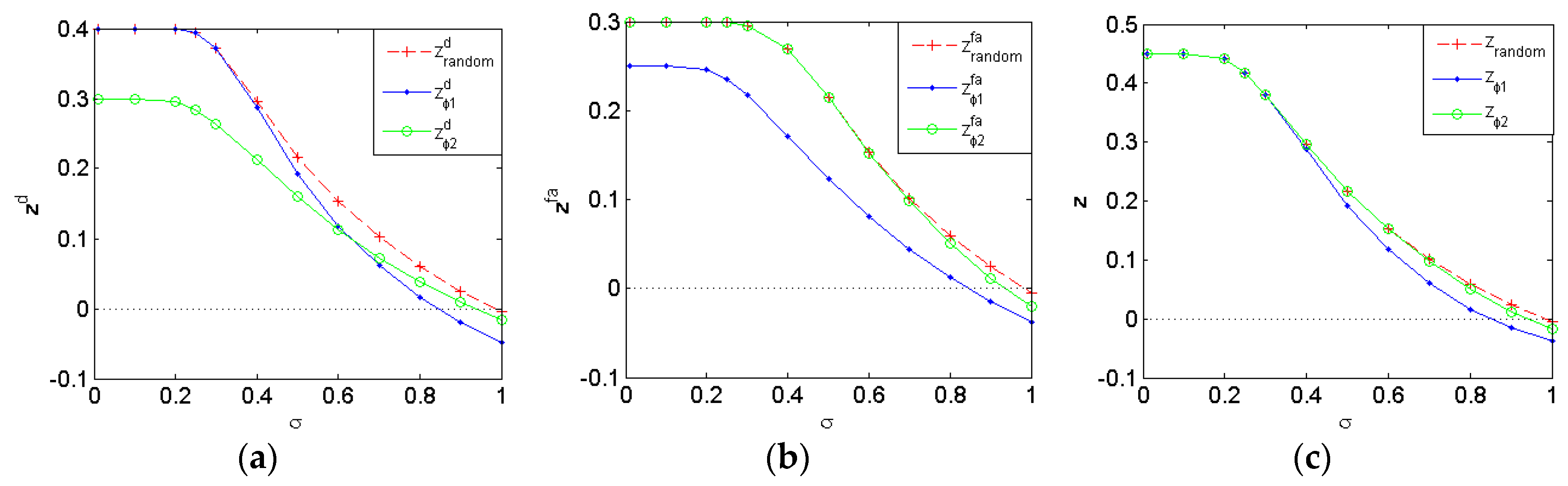
Compared Figure 3 and Figure 1, as $\alpha$ decreases from 0.3 to 0.2, some $z_{\varphi }^{fa}(\mathit{v})$ will change from positive to negative, i.e., the distribution of $(\varphi ,\mathit{v})$ changes. Consequently, for any $\sigma$, there may be some $(\varphi ,\mathit{v})\in M_1$ change to $M_2$ and $M_4$, $(\varphi ,\mathit{v})\in M_2$ change to $M_4$, or $(\varphi ,\mathit{v})\in M_3\cup M_5$ change to $M_6$. As shown in Figure 3a, when $\sigma$ closes to 0, the maximum available $z^d$ for ${\varphi }_1$, ${\varphi }_2$ and the case of allowing the randomization between them are 0.2, 0.15 and 0.25, and the corresponding maximum $P_D^y$ can reach 0.9, 0.85 and 0.95, respectively. As $\sigma$ increases, the maximum $z^d$ for ${\varphi }_1$, ${\varphi }_2$ and the case of allowing the randomization decrease, where the maximum $z^d$ decreases fastest for ${\varphi }_1$ and slowest for ${\varphi }_2$. Further, the maximum achievable $P_D^y$ for ${\varphi }_2$ is greater than that for ${\varphi }_1$ when $\sigma >0.32$ and the difference between the maximum $z^d$ for ${\varphi }_2$ and the case of allowing the randomization are smaller and smaller with the increase of $\sigma$. Compared Figure 3b and Figure 1b, both of them plot the $z^{fa}$ corresponding to the minimum $P_{FA}^y$ under the constraint $P_D^y\ge 0.7$. Especially, $Q_z\subset M_4\cup M_5$ for any $\sigma$, i.e., $z_{opt}=\max (z_{opt}^d,z_{opt}^{fa})$ according to Corollary 3. In addition, compared with Figure 1, under the two constraints that $P_{FA}^y\le \alpha$ and $P_D^y\ge \beta$, the feasible ranges of $\sigma$ for ${\varphi }_1$, ${\varphi }_2$ and the case of allowing the randomization between them become smaller.

In conclusion, as $\sigma$ decreases, the values of $z^d$, $z^{fa}$ and $z$ increase. This is mainly on account of the noise enhanced phenomenon generally occurs when the observation has multimodal pdf and the multimodal structure is more obvious for a smaller $\sigma$ [21]. In order to investigate the simulation results of Figure 1, Figure 2 and Figure 3 further, Table 1, Table 2 and Table 3 present the optimal noise enhanced solutions to maximize $z^d$, $z^{fa}$ and $z$ for ${\varphi }_1$, ${\varphi }_2$ and the case of allowing the randomization, respectively, for different $\sigma$ when $\alpha =0.3$ and $\beta =0.7$.

Table 1. The optimal additive noises to maximize $z^d$, $z^{fa}$ and $z$ for various values of $\sigma$ for ${\varphi }_1$ when $\alpha =0.3$ and $\beta =0.7$.

$\sigma$	$\max z^d$	$\max z^{fa}$	$\max z$
	${\mathit{v}}_1$/${\mathit{v}}_2$/$\lambda$	${\mathit{v}}_1$/${\mathit{v}}_2$/$\lambda$	${\mathit{v}}_1$/${\mathit{v}}_2$/$\lambda$
0.01	[2.5, 2.5]/-/1	[2.5, 2.5]/[−3.75, 2.5]/0.4	[2.5, 2.5]/-/1
0.2	[2.7, 2.75]/-/1	[2.5, 2.5]/[2.7, −3.5]/0.4088	[2.55, 2.5]/-/1
0.4	[2.5, 2.5]/[−3.5, 2.75]/0.9794	[2.5, 2.5]/[−3.5, 2.75]/0.5684	[2.5, 2.5]/[−3.5, 2.75]/0.9794
0.65	-	-	-

Table 2. The optimal additive noises to maximize $z^d$, $z^{fa}$ and $z$ for various values of $\sigma$ for ${\varphi }_2$ when $\alpha =0.3$ and $\beta =0.7$.

$\sigma$	$\max z^d$	$\max z^{fa}$	$\max z$
	${\mathit{v}}_1$/${\mathit{v}}_2$/$\lambda$	${\mathit{v}}_1$/${\mathit{v}}_2$/$\lambda$	${\mathit{v}}_1$/${\mathit{v}}_2$/$\lambda$
0.01	[−5.75, 2.75]/[−3.5, −3.25]/0.6	[−3.75, −3.75]/-/1	[−3.7, −3.75]/-/1
0.2	[2.55, 2.5]/[2.7, −3.5]/0.4088	[−3.7, −3.75]/-/1	[−3.55, −3.5]/-/1
0.4	[−3.75, 2.5]/[−3.5, −3.5]/0.4316	[−3.75, 2.5]/[−3.5, −3.5]/0.0206	[−3.75, 2.5]/[−3.5, −3.5]/0.0206
0.65	-	-	-

Table 3. The optimal additive noises to maximize $z^d$, $z^{fa}$ and $z$ for various values of $\sigma$ for the case of allowing the randomization between ${\varphi }_1$ and ${\varphi }_2$ when $\alpha =0.3$ and $\beta =0.7$.

$\sigma$	$\max z^d$	$\max z^{fa}$	$\max z$
	$(\varphi ,{\mathit{v}}_1)$/-/$\lambda$	$(\varphi ,{\mathit{v}}_1)$/$(\varphi ,{\mathit{v}}_2)$/$\lambda$	$(\varphi ,{\mathit{v}}_1)$/$(\varphi ,{\mathit{v}}_2)$/$\lambda$
0.01	$({\varphi }_1,$ [2.3, 2.75])/-/1	-/$({\varphi }_2,$ [−3.35, −3.25])/1	$({\varphi }_1,$ [2.3, 2.75])/-/1
0.2	$({\varphi }_1,$ [2.75, 2.75])/$({\varphi }_1,$[2.7, 2.75])/0.4770	$({\varphi }_2,$ [−3.7, −3.75])/$({\varphi }_2,$[−3.75, −3.75])/0.5230	-/$({\varphi }_2,$ [−3.55, −3.5])/1
0.4	$({\varphi }_1,$ [2.6, 2.5])/$({\varphi }_2,$[−3.6, −3.5])/0.9141	$({\varphi }_1,$ [2.6, 2.5])/$({\varphi }_2,$[−3.6, −3.5])/0.0859	$({\varphi }_1,$ [2.6, 2.5])/$({\varphi }_2,$ [−3.6, −3.5])/(0.0859, 0.9141)
0.65	$({\varphi }_1,$ [2.65, 2.75])/$({\varphi }_2,$ [−3.65, −3.75])/0.5437	$({\varphi }_1,$[2.65, 2.75])/$({\varphi }_2,$[−3.65, −3.75])/0.4563	$({\varphi }_1,$ [2.65, 2.75])/$({\varphi }_2,$ [−3.65, −3.75])/(0.4563, 0.5437)

It is worthy to note that the optimal noise enhanced solutions to maximize $z^d$, $z^{fa}$ and $z$, respectively, are not unique in many cases. Moreover, due to the property of the detector, the noise modified detectability for ${\varphi }_i$, $i=1,2$, obtained by adding $\mathit{v}={(v_1,v_2)}^T$ is the same with that achieved via adding $\mathit{v}={(v_2,v_1)}^T$. As a demonstration, for each $\sigma$, there only lists one noise enhanced solution for the maximum $z^d$, as well as the maximum $z^{fa}$ and $z$. As shown in Table 1, Table 2 and Table 3, the optimal noise enhanced solutions to maximize $z^d$, $z^{fa}$ and $z$, respectively, are the randomization of at most two detector and discrete vector pairs $({\varphi }_1,{\mathit{v}}_1)$ and $({\varphi }_2,{\mathit{v}}_2)$ from two different sets, which are consistent with Theorems 1–3.

Next, the noise enhanced solution for ${\varphi }_1$ is taken as an example to illustrate firstly. When $\sigma =0.01$, the maximum $z_{{\varphi }_1}^d(\mathit{v})$ obtained by $({\varphi }_1,\mathit{v})\in M_{1,{\varphi }_1}$ is equal to the maximum $z_{{\varphi }_1}^d(\mathit{v})$ obtained by $({\varphi }_1,\mathit{v})\in M_{{\varphi }_1}$.Through some calculations, $\mathit{v}=[2.5,2.5]\in M_{1,{\varphi }_1}$ is one of the discrete vectors to maximize $z_{{\varphi }_1}^d(\mathit{v})$, so $\mathit{v}=[2.5,2.5]$ is the optimal noise to maximize $z^d$ for ${\varphi }_1$ when $\alpha =0.3$ and $\beta =0.7$. At the same time, the $z_{{\varphi }_1}(\mathit{v})$ obtained by $\mathit{v}=[2.5,2.5]$ is also the maximum $z_{{\varphi }_1}(\mathit{v})$ for ${\varphi }_1$, thus $\mathit{v}=[2.5,2.5]$ is the optimal noise to maximize $z$ for ${\varphi }_1$. Besides, the maximum $z_{{\varphi }_1}^{fa}(\mathit{v})$ obtained from $M_{1,{\varphi }_1}$ and $M_{3,{\varphi }_1}$ are smaller than the maximum $z_{{\varphi }_1}^{fa}(\mathit{v})$ for ${\varphi }_1$, then the maximum $z^{fa}$ under the two constraints $P_{FA}^y\le 0.3$ and $P_D^y\ge 0.7$ is obtained by the randomization of ${\mathit{v}}_1=[2.5,2.5]$ from $M_{1,{\varphi }_1}$ and ${\mathit{v}}_2=[-3.75,2.5]$ from $M_{5,{\varphi }_1}$ with probabilities 0.4 and 0.6, respectively. The case of $\sigma =0.2$ is similar with the case of $\sigma =0.01$.

When $\sigma =0.4$, both $M_{2,{\varphi }_1}$ and $M_{3,{\varphi }_1}$ are null, and the maximum $z_{{\varphi }_1}^d(\mathit{v})$, $z_{{\varphi }_1}^{fa}(\mathit{v})$ and $z_{{\varphi }_1}(\mathit{v})$ for ${\varphi }_1$ cannot be obtained by the discrete vector from $M_{1,{\varphi }_1}$. Based on Theorems 1–3, the maximum $z^d$, $z^{fa}$ and $z$ can be achieved by the randomization of two detector and discrete vector pairs from $M_{4,{\varphi }_1}$ and $M_{5,{\varphi }_1}$. Further, the noise enhanced solutions for the maximum $z^d$ and $z^{fa}$ have the same additive noise components, i.e., ${\mathit{v}}_1$ and ${\mathit{v}}_2$, but with different probabilities. Moreover, according to Corollary 3(b), $z_{opt}=\max (z_{opt}^d,z_{opt}^{fa})$. When the randomization between ${\varphi }_1$ and ${\varphi }_1$ is allowed, the $z_{{\varphi }_1}({\mathit{v}}_1)$ obtained by $({\varphi }_1,{\mathit{v}}_1=[2.6,2.5])\in M_4$ is equal to the $z_{{\varphi }_2}({\mathit{v}}_2)$ obtained by $({\varphi }_2,{\mathit{v}}_2=[-3.6,-3.5])\in M_5$, and it is the maximum $z_{\varphi }(\mathit{v})$ obtained in $M$. According to Corollary 3(c), the maximum $z^d$, $z^{fa}$ and $z$ can be obtained by the randomization of $({\varphi }_1,{\mathit{v}}_1)$ and $({\varphi }_2,{\mathit{v}}_2)$ with different probabilities. Especially, the probability $\lambda$ of $({\varphi }_1,{\mathit{v}}_1)$ for the maximum $z^d$ or $z^{fa}$ is unique, while the probability $\lambda$ of $({\varphi }_1,{\mathit{v}}_1)$ for the maximum $z$ can be chosen in a certain interval. When $\sigma =0.65$, no noise enhanced solution exists to meet the two constraints for the nonrandomization case in Table 1 and Table 2, while there still exist noise enhanced solutions to improve the detectability under the same constraints by allowing randomization between ${\varphi }_1$ and ${\varphi }_2$ shown in Table 3 and the corresponding solutions are also obtained according to Corollary 3(c).

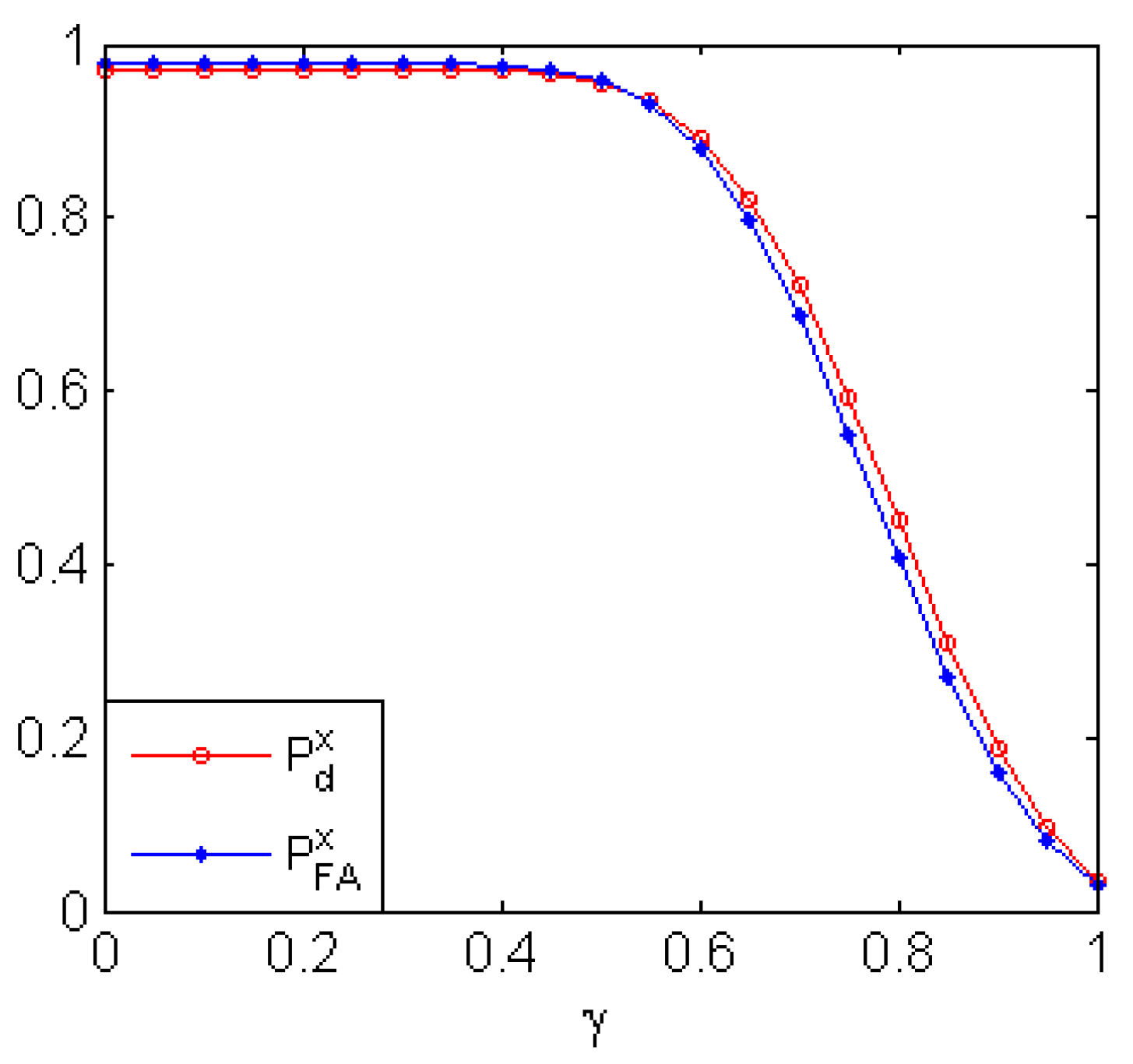
In order to discuss the effect of the decision threshold $\gamma$ on the detection and false-alarm probabilities, the proposed noise enhanced method is operated on different values of $\gamma$. Further, the relationships between the maximum achievable detection probability and $\beta$, the minimum achievable false-alarm probability and $\alpha$ are explored for different $\gamma$. The different results of the original detector and the noise enhanced detector for different $\gamma$ are given in Figure 4, Figure 5 and Figure 6.

Figure 4. $P_D^x$ and $P_{FA}^x$ for different $\gamma$ when $\mu =3$, $A=1$, $\sigma =1$ and $K=20$.

Figure 5. The maximum achievable $P_D^y$ as a function of. for $\gamma =0.05,0.25,0.5,0.75$ and $0.95$, and the case of allowing the randomization between thresholds, when $\mu =3$, $A=1$, $\sigma =1$ and $K=20$.

Figure 6. The minimum achievable $P_{FA}^y$ as a function of $\beta$ for $\gamma =0.05,0.25,0.5,0.75$ and $0.95$, and the case of allowing the randomization between thresholds, when $\mu =3$, $A=1$, $\sigma =1$ and $K=20$.

Figure 4 gives the original detection and false-alarm probabilities for different $\gamma$ when $K=20$. From Figure 4, we can see that both the original detection and false-alarm probabilities decrease with the increase of $\gamma$ and the value of the original detection probability is close to that of the original false-alarm probability for any $\gamma$. In other words, a better detection probability is obtained for a smaller $\gamma$ and a lower false-alarm probability is achieved for a greater $\gamma$. 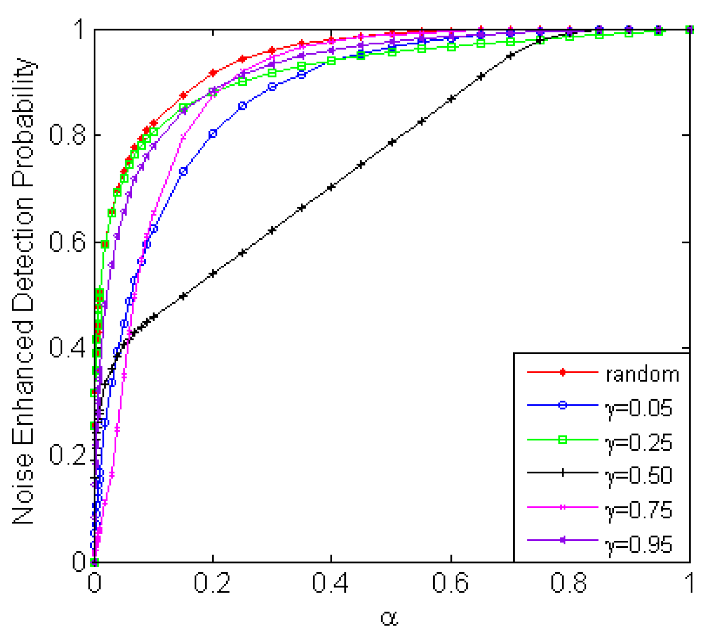Figure 5 plots the maximum achievable $P_D^y$ obtained by adding noise as a function of $\alpha$ for $\gamma =0.05,0.25,0.5,0.75$ and $0.95$, and the case of allowing the randomization between thresholds, when $\mu =3$, $A=1$, $\sigma =1$ and $K=20$. Compared Figure 5 with Figure 4, the detection probabilities for $\gamma =0.95$ and 0.75 can be increased significantly by adding suitable additive noises with a lower false-alarm probability. 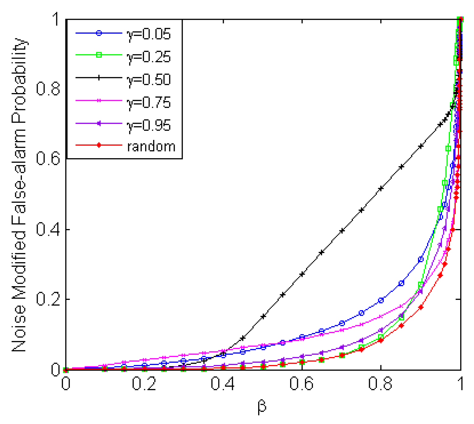Figure 6 presents the minimum achievable $P_{FA}^y$ obtained by adding noise as a function of $\beta$ for $\gamma =0.05,0.25,0.5,0.75$ and $0.95$, and the case of allowing the randomization between thresholds, when $\mu =3$, $A=1$, $\sigma =1$ and $K=20$. Comparing Figure 6 with Figure 4, the false-alarm probabilities for $\gamma =0.05$, 0.25 and 0. 5 can be decreased significantly by adding suitable additive noises with a higher detection probability. From Figure 5 and Figure 6, different detection performance can be realized by adding noise. As shown in Figure 5 and Figure 6, for the cases of $\alpha \in (0.055,0.725)$ and $\beta \in (0.405,0.975)$, the detector of $\gamma =0.5$ shows the worst performance compared to others. Thus, in such cases, $\gamma =0.5$ is not a suitable threshold. From Figure 5 and Figure 6, different detection performance can be realized by adding noises. Namely, various noise enhanced solutions can be provided with our method to satisfy different performance requirements. As a result, for any decision threshold $\gamma$, we can determine whether the performance of the detector can be improved or not, and search a noise enhanced solution to realize the improvement according to the method proposed in this paper.

It is worthy to note that there is no limit on the detector in the method proposed in this manuscript. Furthermore, it only depends on detector itself whether the detection performance of the detector can or cannot be improved by adding noise. The algorithms proposed in this paper not only provide ways to prove the improvability or nonimprovability, but also analyze how to search the optimal noise enhanced solutions. For any detector, no matter an optimal Neyman–Pearson (Bayesian, Minimax) detector or other suboptimal detector, we first calculate all information of $(P_{D,{\varphi }_{\ell }}(\mathit{v}),P_{FA,{\varphi }_{\ell }}(\mathit{v}))$ obtained by every detector and discrete vector pair $({\varphi }_{\ell },\mathit{v})$. Then, we divide each pair $({\varphi }_{\ell },\mathit{v})$ into six sets according to the values of $z_{{\varphi }_{\ell }}^d(\mathit{v})$ and $z_{{\varphi }_{\ell }}^{fa}(\mathit{v})$, where $z_{{\varphi }_{\ell }}^d(\mathit{v})=P_{D,{\varphi }_{\ell }}^y(\mathit{v})-\beta$ and $z_{{\varphi }_{\ell }}^{fa}(\mathit{v})=\alpha -P_{FA,{\varphi }_{\ell }}^y(\mathit{v})$. If there exist detector and discrete vector pairs to satisfy the sufficient conditions as given in Section 3.4, noise enhanced solutions to maximize $z^d$, $z^{fa}$ and $z$ can be obtained according to Section 3.1, Section 3.2, and Section 3.3, respectively, on the premise that $P_D^y\ge \beta$ and $P_{FA}^y\le \alpha$. Otherwise, no noise enhanced solution exists to satisfy $P_D^y\ge \beta$ and $P_{FA}^y\le \alpha$ simultaneously.

5. Conclusions

In this paper, a framework consisting of six mutually disjoint sets is established according to two inequality-constraints on detection and false-alarm probabilities. The maximization of $z^d$, $z^{fa}$ and $z$ are searched based on the framework. Theorems 1–3 give the forms of the optimal noise enhanced solutions to maximize $z^d$, $z^{fa}$ and $z$. The calculations of maximum $z^d$, $z^{fa}$ and $z$ are presented in Corollaries 1, 2 and 3, respectively. Especially, the maximum $z$ is equal to the maximum $z^d$ or $z^{fa}$ under certain conditions according to Corollary 3. Furthermore, sufficient conditions for $P_D^y\ge \beta$ and $P_{FA}^y\le \alpha$ are given in Theorem 4.

Compared with the method proposed in [16], which only focuses on the maximization of $z^d$ with a constant false-alarm rate (CFAR), both methods require all the information of $(P_{D,{\varphi }_{\ell }}(\mathit{v}),P_{FA,{\varphi }_{\ell }}(\mathit{v}))$ obtained by every detector and discrete vector pair $({\varphi }_{\ell },\mathit{v})$, and our method may use the information more effectively to realize the overall improved performance or decrease the false alarm probability due to the division of six sets.

Furthermore, the theoretical results in this paper can be extended to a broad class of noise enhanced optimal problems subject to two inequality constraints, such as the minimization of Bayes risk under the constraint on condition risk about the binary hypothesis testing problem, and the minimization of linear combinations of error probabilities under constraints on type I and II error probabilities as discussed in [28].