Quantum Coherent Three-Terminal Thermoelectrics: Maximum Efficiency at Given Power Output

Abstract

This work considers the nonlinear scattering theory for three-terminal thermoelectric devices used for power generation or refrigeration. Such systems are quantum phase-coherent versions of a thermocouple, and the theory applies to systems in which interactions can be treated at a mean-field level. It considers an arbitrary three-terminal system in any external magnetic field, including systems with broken time-reversal symmetry, such as chiral thermoelectrics, as well as systems in which the magnetic field plays no role. It is shown that the upper bound on efficiency at given power output is of quantum origin and is stricter than Carnot’s bound. The bound is exactly the same as previously found for two-terminal devices and can be achieved by three-terminal systems with or without broken time-reversal symmetry, i.e., chiral and non-chiral thermoelectrics.

1. Introduction

Thermodynamics was the great product of nineteenth century physics; it is epitomized by the concept that there is an upper bound on the efficiency of any thermodynamic machine, known as the Carnot limit. This concept survived the quantum revolution with little more than a scratch; at present, few physicists believe that a quantum machine can produce a significant amount of work at an efficiency exceeding the Carnot limit. Of course, both statistical mechanics and quantum mechanics exhibit fluctuations, and these fluctuations may violate Carnot’s limit on short timescales. However, these fluctuations average out on longer timescales, so it is believed that any quantum machine left running long enough to produce a non-microscopic amount of work will not exceed the Carnot limit. However, this work will consider the limit where the work output is large enough that such fluctuation effects are negligible. In this limit it is generally believed that Carnot’s limit is only achievable for vanishing power output, even if there is no general proof of this. It was recently observed for two-terminal thermoelectric machines that quantum mechanics imposes a stricter upper bound on the efficiency at finite power output [1,2]. This upper bound coincides with that of Carnot at vanishing power output, but decays monotonically as one increases the desired power output.

In recent years, there has been a lot of theoretical [3,4,5,6,7,8,9,10,11,12,13,14,15,16,17,18,19,20] and experimental [21,22,23] interest in three-terminal thermoelectrics (see Figure 1). In particular, it is suggested that chiral three-terminal thermoelectrics [18,19,20] could have properties of great interest for efficient power generation. Most of these three-terminal systems are quantum versions of traditional thermocouples [24,25,26,27], since they have one terminal in contact with a thermal reservoir and two terminals in contact with electronic reservoirs (see Figure 1). They turn heat flow from the thermal reservoir into electrical power in the electronic reservoirs, or vice versa. I refer to such three-terminal systems as quantum thermocouples, since they are too small to be treated with the usual Boltzmann transport theory. There are two quantum lengthscales which enter into consideration: the electron’s wavelength and its decoherence length. In this work, I will be interested in devices in which the whole thermocouple is much smaller than the decoherence length [9,10,15,16,17,18,19]. Such thermocouples would typically be larger than the electron wavelength, although they need not be. The crucial point is that electrons flow elastically (without changing energy or thermalizing) through the central region in Figure 1a. This can also be a simple phenomenological model of the system in Figure 1c ( see Section 1.4). In these systems, quantum interference effects can have a crucial effect on the physics. Such phase-coherent transport effects are not captured by the usual Boltzmann transport theory, but they can be modeled using Christen and Büttiker’s nonlinear scattering theory [28], in the cases where it is acceptable to treat electron–electron interactions at the mean-field level. Such three-terminal systems are about the simplest self-contained quantum machines.

Reservoir M is taken to supply heat to the system but not electrical current. Thus, the heat current into the system from reservoir M ($J_{\mathrm{M}}$) is finite, while the electrical current into the system from reservoir M obeys

$$\begin{array}{c}{I}_{\mathrm{M}}=0\hfill \end{array}$$

(1)

(see Figure 2). If reservoir L and R are at the same temperature $T_0$, and reservoir M is hotter at $T_{\mathrm{M}}>T_0$, one can use the heat flow $J_{\mathrm{M}}$ to drive an electrical current from L to R. If this electrical current flows against a potential difference, then the system turns heat into electrical power, and so is acting as a thermodynamic heat-engine. Alternatively, one can make the system act as a refrigerator, by applying a bias which drives a current from L to R, and “sucks” heat out of a reservoir M (Peltier cooling) taking it to a lower temperature than reservoirs L and R, $T_{\mathrm{M}}<T_0$.

This work considers arbitrary phase-coherent three-terminal quantum systems that fall in to the category described by Christen and Buttiker’s nonlinear scattering theory [28]. I find upper bounds on such a system’s efficiency as a heat-engine or a refrigerator at finite power output. These bounds coincide with those of two-terminal quantum systems considered in [1,2], irrespective of whether the three-terminal system’s time-reversal symmetry is broken (by an external magnetic field) or not. Thus, these bound applies equally to normal and chiral thermoelectrics [18,19,20].

1.1. The Carnot Bound

When the system acts as a heat-engine (or energy-harvester [29,30]), the input is the heat current coming from the thermal reservoir (reservoir M), $J_{\mathrm{M}}$, and the output is the electrical power generated by the system, $P_{\mathrm{gen}}$. This power flows into a load attached between reservoirs L and R; this load could be a motor turning electrical work into mechanical work, or some sort of work storage device. The heat-engine (eng) efficiency is defined as:

$$\begin{array}{c}{\eta }_{\mathrm{eng}}=P_{\mathrm{gen}}/J_{\mathrm{M}}.\hfill \end{array}$$

(2)

This never exceeds Carnot’s limit,

$$\begin{array}{ccc}{\eta }_{\mathrm{eng}}^{\mathrm{Carnot}}\hfill & =& 1-T_0/T_{\mathrm{M}},\hfill \end{array}$$

(3)

where we recall that $T_{\mathrm{M}}>T_0$. For the refrigerator, the situation is reversed, the load is replaced by a power supply, and the system absorbs power, $P_{\mathrm{abs}}$, from that supply. The cooling power output is the heat current that is “sucked” out of the colder reservoir (reservoir M), $J_{\mathrm{M}}$. Thus, the refrigerator (fri) efficiency or coefficient of performance (COP) is,

$$\begin{array}{c}{\eta }_{\mathrm{fri}}=J_{\mathrm{M}}/P_{\mathrm{abs}}.\hfill \end{array}$$

(4)

This never exceeds Carnot’s limit,

$$\begin{array}{ccc}{\eta }_{\mathrm{fri}}^{\mathrm{Carnot}}\hfill & =& {(T_0/T_{\mathrm{M}}-1)}^{-1},\hfill \end{array}$$

(5)

where we have $T_{\mathrm{M}}<T_0$ (which is the opposite of heat-engine). These Carnot limits are the upper bound on efficiency of heat-engines and refrigerators. It has often been argued that Carnot efficiency is only achievable at zero cooling power, but no general proof of this claim exists (see Section 1.3).

1.2. Stricter Upper Bound for Two-Terminal Systems

Bekenstein [31,32] and Pendry [33] independently noted that there is an upper bound on the heat that can flow through a single transverse mode. As a result, the heat that any wave (electron, photon, etc.) can carry away from reservoir i at temperature $T_i$ through a cross-section carrying N transverse modes is

$$\begin{array}{c}{J}_{\mathrm{i}}^{\mathrm{qb}}=\frac{{\pi }^2}{6h}N{k}_{\mathrm{B}}^2{T}_i^2,\hfill \end{array}$$

(6)

where the number of transverse modes is of the order of the cross-section in units of the wavelength of the particles carrying the heat. This Bekenstein–Pendry bound was observed experimentally in point-contacts [34], and was recently verified to high accuracy in quantum Hall edge-states [35].

References [1,2] pointed out that this upper bound on heat flow must place a similar upper bound on the power generated by a heat-engine (since the efficiency is always finite). Those works used the nonlinear version of Landauer scattering theory [28] to find this upper bound on the power generated, which they called the quantum bound (qb), since its originates from the wavelike nature of electrons in quantum mechanics. It takes the form

$$\begin{array}{c}{P}_{\mathrm{gen}}^{\mathrm{qb}}\equiv A_0\frac{{\pi }^2}{h}N{k}_{\mathrm{B}}^2{\left(T_L-T_R\right)}^2,\hfill \end{array}$$

(7)

where $A_0\simeq 0.0321$. References [1,2] then calculated the upper bound on a heat engine’s efficiency for given power generation $P_{\mathrm{gen}}$, and showed that it is a monotonically decaying function of $P_{\mathrm{gen}}/P_{\mathrm{gen}}^{\mathrm{qb}}$. There is no closed form algebraic expression for this upper bound at arbitrary $P_{\mathrm{gen}}/P_{\mathrm{gen}}^{\mathrm{qb}}$, and it is given by the solution of a transcendental equation. However, for $P_{\mathrm{gen}}/P_{\mathrm{gen}}^{\mathrm{qb}}\ll 1$, the maximum efficiency at power $P_{\mathrm{gen}}$ is

$$\begin{array}{c}{\eta }_{\mathrm{eng}}\left(P_{\mathrm{gen}}\right)={\eta }_{\mathrm{eng}}^{\mathrm{Carnot}}\left(1-0.478\sqrt{\frac{T_R}{T_L}\frac{P_{\mathrm{gen}}}{P_{\mathrm{gen}}^{\mathrm{qb}}}}+\mathcal{O}\left[P_{\mathrm{gen}}/P_{\mathrm{gen}}^{\mathrm{qb}}\right]\right).\hfill \end{array}$$

(8)

Thus, one can only achieve Carnot efficiency at vanishing power generation, $P_{\mathrm{gen}}\to 0$, although one comes close to Carnot efficiency for $P_{\mathrm{gen}}\ll P_{\mathrm{gen}}^{\mathrm{qb}}$.

In the limit of maximum power generation, $P_{\mathrm{gen}}=P_{\mathrm{gen}}^{\mathrm{qb}}$, the upper bound on efficiency is

$$\begin{array}{ccc}{\eta }_{\mathrm{eng}}\left(P_{\mathrm{gen}}^{\mathrm{qb}}\right)\hfill & =& \frac{{\eta }_{\mathrm{eng}}^{\mathrm{Carnot}}}{1+0.936(1+T_R/T_L)}.\hfill \end{array}$$

(9)

References [1,2] calculated similar expressions for the upper bound on refrigerator efficiency as a function of cooling power. In this case, the upper bound is found to be half the Bekenstein–Pendry bound on heat-flow. Again, the maximum efficiency equals that of Carnot for cooling powers much less than the Bekenstein–Pendry bound and decays monotonically as one increases the desired cooling power towards its upper limit.

In the naive classical limit of vanishing wavelength compared to system size, one has $N\to \infty$, and so the quantum bound $P_{\mathrm{gen}}^{\mathrm{qb}}$ and $J_i^{\mathrm{qb}}$ becomes irrelevant (they go to infinity). Thus, in this limit, it appears that one can achieve Carnot efficiency for any power output. However, quantum mechanics says that this is not the case, that, for any power output that is a significant fraction of $P_{\mathrm{gen}}^{\mathrm{qb}}$ or $J_i^{\mathrm{qb}}$, the upper bound on efficiency is lower than Carnot efficiency. This efficiency bound was derived for two-terminal quantum systems, and here I will show that exactly the same bounds apply to three-terminal quantum systems.

1.3. Universality of This Bound?—A Brief Literature Review

The upper bound on efficiency at given power has been of some interest recently. Various results have been derived in various regimes, and the complexity of these calculations means that there is not yet a consensus about how to compare these results. Here, I attempt such a comparison, taking the risk that I may have misunderstood some of these complexities.

Many textbooks on thermodynamics give some sort of handwaving argument saying that a heat-engine exhibiting Carnot efficiency has a vanishing power output, but this is by no means proven. In the specific context of the Carnot cycle, a step in this direction was made in the the pedagogical work of Curzon and Ahlborn [36] (although their result was found earlier [37,38,39]), which gave a curve for the efficiency as a function of the power of the machine, and discussed in detail the efficiency at that machine’s maximum power, $P_{\mathrm{m}}$. In the linear response regime, one can use Onsager’s non-equilibrium thermodynamics to show that this curve is particularly simple, and it takes the form [40] $\eta \left(P_{\mathrm{gen}}\right)=\frac{1}{2}{\eta }_{\mathrm{eng}}^{\mathrm{Carnot}}\left(1+\sqrt{P_{\mathrm{gen}}/P_{\mathrm{m}}}\right)$ (see also references [8,9,10,41]). This goes linearly with $P_{\mathrm{gen}}$ when $P_{\mathrm{gen}}$ is small, rather than like a squareroot as in Equation (8). However, a much bigger difference is that the theory does not give a value for $P_{\mathrm{m}}$, nor does it give an upper bound on $P_{\mathrm{m}}$. As a result, such relations imply that one could get arbitrarily close to Carnot efficiency at any finite power, $P_{\mathrm{gen}}$, by building a machine with $P_{\mathrm{m}}\to \infty$. For refrigerators, reference [42] showed that the entropy production rate goes like the power squared with a prefactor that goes like $L_{\mathrm{qq}}/L_{\rho \mathrm{q}}^2$, where $L_{\mu \nu }$ is an Onsager coefficient with $\mu ,\nu \in \rho$(charge)$,q$(heat). However, without a lower bound on $L_{\mathrm{qq}}/L_{\rho \mathrm{q}}^2$ (which may be power dependent), this does not give us a lower bound on the entropy production rate at given refrigerator power (such a lower bound would correspond to an upper bound on efficiency via Equation (56)). I believe that it is quantum mechanics that gives the upper bounds on $P_{\mathrm{m}}$ (and on lower bound on $L_{\mathrm{qq}}/L_{\rho \mathrm{q}}^2$), and so it is absent from these classical theories.

The first results that indicated the importance of quantum mechanics were those that used scattering theory to show that Carnot efficiency required vanishingly narrow transmission functions in both the linear [43] and nonlinear regimes [44,45] (reference [43] actually used the Boltzmann transport theory, but every step of their calculation can be recast in terms of scattering theory if desired). A natural consequence of a vanishingly narrow transmission function is that the proportion of electrons that transmit through the thermoelectric structure is vanishingly small. This implies that the power output of such a system is vanishingly small for such a system irrespective of the bias one chooses. More strictly, this power output vanishes for any finite sized system (i.e., any system with a finite number of transverse modes). Formally, one can get a finite power in the limit, if one allows the machine’s cross-section to diverge as one takes the transmission function’s width to zero, but this is unphysical and is not considered further here.

In the linear-response language, these works tell us that the system whose figure of merit $ZT\equiv G{S}^{2}T/K\to \infty$ (Carnot efficiency requires $ZT\to \infty$), has Onsager coefficient $L_{\mu \nu }$ whose magnitude’s vanishes for all $\mu ,\nu$, while the Seebeck coefficient $S\propto L_{\rho \mathrm{q}}/L_{\rho \rho }$ remains finite, and the Weidemann–Franz ratio $K/\left(GT\right)\propto \left(L_{\rho \rho }{L}_{\mathrm{qq}}-L_{\rho \mathrm{q}}{L}_{\mathrm{q}\rho }\right)/L_{\rho \rho }^2$ vanishes. Even if one chooses the load to maximize the power output, giving a power $P_{\mathrm{m}}$, the fact the transmission function is vanishingly narrow means that $P_{\mathrm{m}}\to 0$. This was the first indication that one could not take a machine’s $P_{\mathrm{m}}$ to be independent of its efficiency.

This brings us to the scattering theory calculation in references [1,2], outlined in the previous section. There, Equation (8) shows that Carnot efficiency is not achievable unless the power output is vanishing, and that the deviation from Carnot efficiency goes like the squareroot of power. This result is primarily for fully coherent transport, but reference [2] also considered a relaxation process within the scatterer as modeled by a fictitious reservoir (in the style of a voltage probe [46,47,48,49]) in the absence of an external magnetic field, and recovered Equation (8) for small $P_{\mathrm{gen}}$. Thus, a natural question is how universal these bounds are. The objective of this work is to show that the bounds in references [1,2] also applies to those relaxation-free three-terminal systems which can be modeled by scattering theory.

However, returning to the effect of relaxation in two-terminal systems, reference [50] considered the linear-response limit of scattering theory with an arbitrary number of fictitious reservoirs to model more complicated relaxation processes (and with an arbitrary external magnetic field). They considered maximizing the power for given efficiency and found a bound that was weakest when the number of fictitious reservoirs goes to infinity. In the limit of small power, their result gives the maximum efficiency for given power as:

$$\begin{array}{c}{\eta }_{\mathrm{eng}}\left(P\right)={\eta }_{\mathrm{eng}}^{\mathrm{Carnot}}\times \left(1-P_{\mathrm{gen}}/\left(4P_0\right)+\cdots \right),\hfill \end{array}$$

(10)

where $P_0$ is the same as $P_{\mathrm{gen}}^{\max }$, except for a difference in the numerical prefactor. The absence of the square-root makes this bound much less strict at small $P_{\mathrm{gen}}$ than Equation (8). This hints that it might be possible to exceed Equation (8) by adding a large amount of relaxation within the scatterer (as modeled by an infinite number of fictitious reservoirs). However, reference [50] say that their upper bound may be an over-estimate; they do not prove it is a tight bound by giving an example of a system that achieves their upper bound. Thus, one cannot yet say for certain whether a system of the type that they propose can violate the bound in Equation (8) or not. Similarly, nothing is known about the bound for systems that are not modeled by scattering theory, such as systems exhibiting strong interaction effects (Coulomb-blockade, Kondo effect, etc). Thus, it remains to be seen how universal this bound is, even if Equation (8) is obeyed by all the systems for which a tight bound has been derived to date.

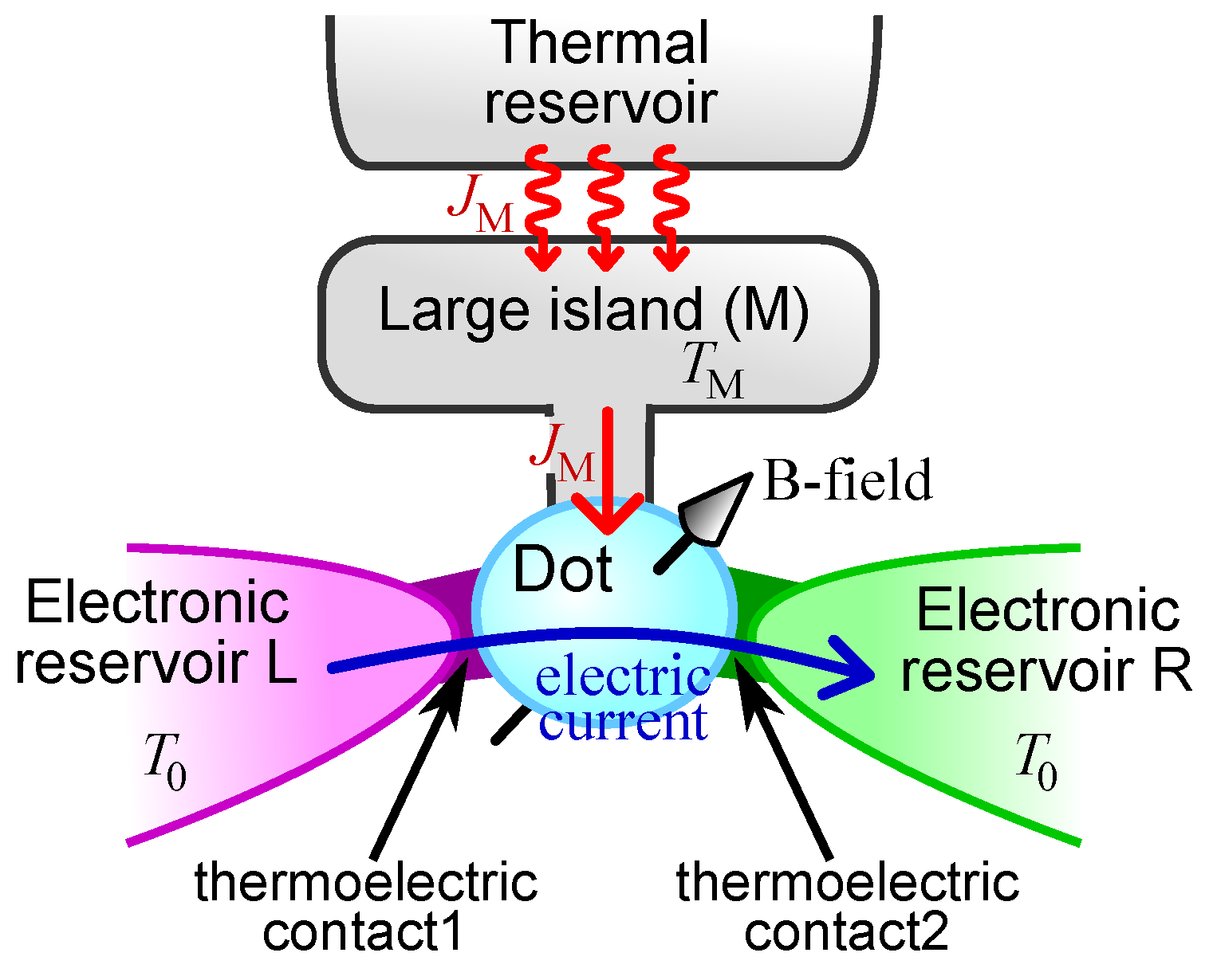
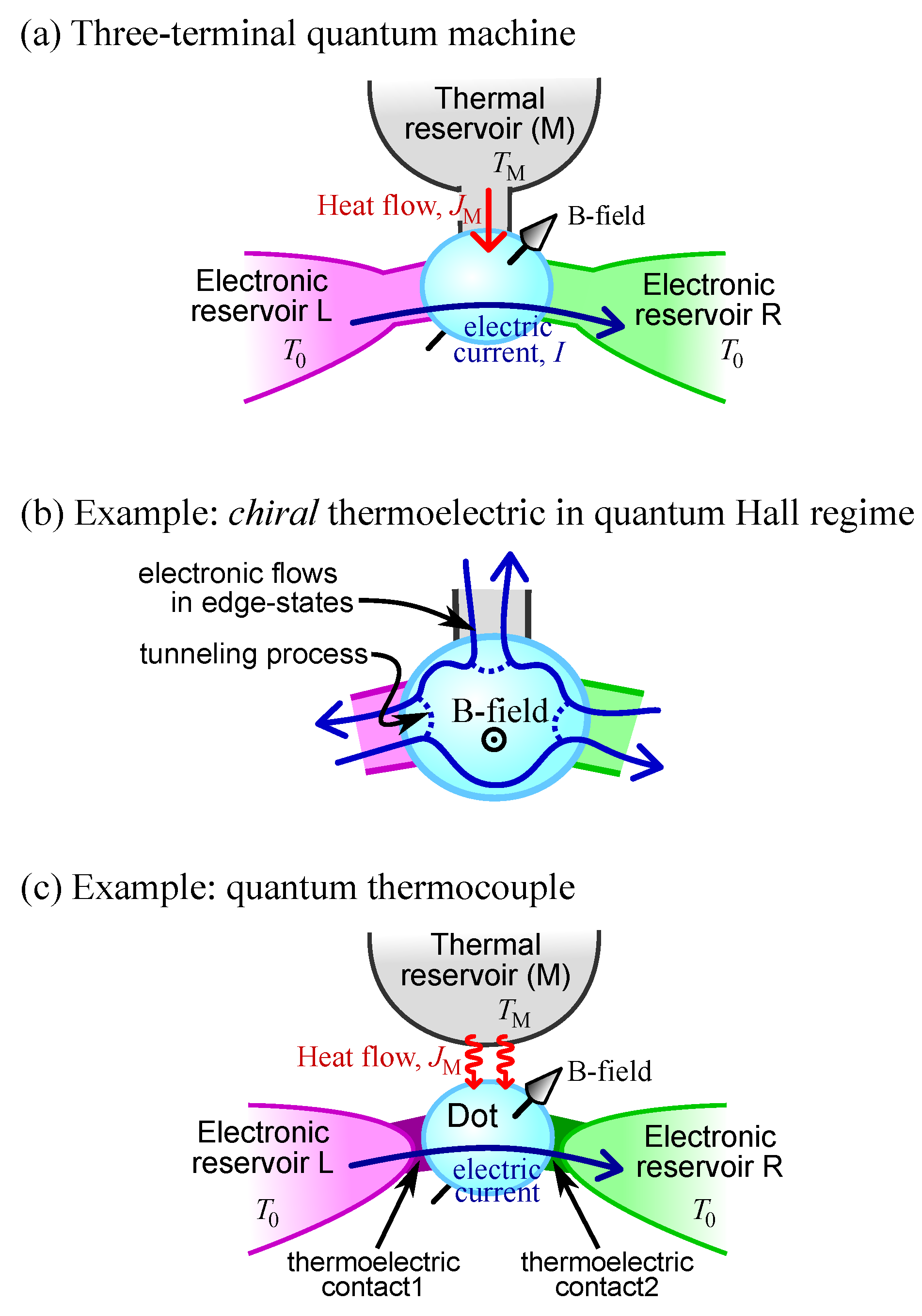
1.4. Examples of Three Terminal Systems: Chiral Thermoelectrics and Quantum Thermocouples

Here, I discuss two examples of systems for which the bounds derived here apply. The first example is the chiral thermoelectric sketched in Figure 1b, as discussed in references [18,19,20]. This is a three-teminal system exposed to such a strong external magnetic field that the electron flow only occurs via edge-states (all bulk states are localized by the magnetic field). These edge-states are chiral, which means they circulate in a preferred direction in the scattering region (anticlockwise in Figure 1b), This is an intriguing situation for a heat-engine in which one wants to generate electrical power by driving a flow of electrons from reservoir L (at lower chemical potential) to reservoir R (at higher chemical potential). The B-field alone generates an electron flow directly from L to R without a corresponding direct electron flow from R to L. Thus, it would seem plausible that one could take advantage of this, with a suitable choice of Reservoir M and of the central scattering region to achieve higher efficiencies than in a two-terminal device (where every flow from L to R has a corresponding flow from R to L). Unfortunately, our general solution for a three-terminal system will show that the upper bound on efficiency at given power output is independent of the external magnetic field, so it is the same for chiral or non-chiral systems.

The second example is the quantum thermocouple sketched in Figure 1c. Here, the third terminal (reservoir M) supplies heat in the form of photons (or phonons). Such systems have been considered using microscopic models of the photon flow [3,4,5,6,7,11,12,14,20]; however, here I instead use a phenomenological argument to replace the reservoir of photons sketched in Figure 1c by the reservoir of electrons sketched in Figure 1a. This is the “voltage probe” model [46,47,48,49], in which inelastic scattering (such as electrons scattering from photons) is modeled by a reservoir of electrons whose chemical potential is chosen such that that, on average, every electron that escapes the system into that reservoir is replaced by one coming into the system from that reservoir, so $I_{\mathrm{M}}=0$. Figure 2 shows a system for which this voltage probe model is correct. The island is large enough that any electron entering it thermalizes at temperature $T_{\mathrm{M}}$ before escaping back into the dot. Since the island is in a steady-state at temperature $T_{\mathrm{M}}$, the heat flow out of the island due to electrons must equal the heat flow into the island due to photons. However, one can also argue phenomenologically that the same model is a simplified description of the system sketched in Figure 1c. This phenomenological model treats the exchange of a photon between the dot and reservoir M as the replacement of an electron in the dot which has the dot’s energy distribution, with an electron which has reservoir M’s energy distribution. Of course, this is not the most realistic model of electron–photon interactions. In particular, it assumes that each electron entering from reservoir L or R either escapes into one of those two reservoirs without any inelastic scattering from the photon-field, or it escapes after undergoing so many scatterings from the photon-field that it has completely thermalized with the photon-field. As such, this model does not capture the physics of electrons that undergo one or two inelastic scatterings from the photon-field before escaping into reservoir L or R. At this simplistic level of modelling, nothing would change if it were phonons rather than photons coming from reservoir M. While this voltage probe model has been successfully used to understand the basics of many inelastic effects in nanostructures, it should not be considered a replacement for a proper microscopic theory (see e.g., references [51,52] for a discussion of how the voltage probe model fails to capture aspects of inelastic scattering in ultra-clean nanostructures). One should be cautious about applying results for a system of the type in Figure 1a to a system of the type in Figure 1c, but it is none the less a reasonable first step to understanding its physics.

2. Electrical and Heat Currents

Consider a system with a scattering matrix, $\mathcal{S}\left(ϵ\right)$, then the transmission matrix for electrons at energy ϵ made of elements

$$\begin{array}{c}{\mathcal{T}}_{ij}\left(ϵ\right)=\mathrm{tr}\left[{\mathcal{S}}_{ij}^{†}\left(ϵ\right){\mathcal{S}}_{ij}\left(ϵ\right)\right],\hfill \end{array}$$

(11)

where the trace is over all transverse modes of leads i and j. The electrical current out of reservoir i is then

$$\begin{array}{c}{I}_i=e^{-}{\int }_{-\infty }^{\infty }\frac{\mathrm{d}ϵ}{h}\sum _j({\mathcal{T}}_{ij}\left(ϵ\right)-N_i\left(ϵ\right){\delta }_{ij})f_j\left(ϵ\right),\hfill \end{array}$$

(12)

where lead i has $N_i\left(ϵ\right)$ modes for particles at energy ϵ, and the Fermi function in reservoir j is defined as

$$\begin{array}{c}{f}_j\left(ϵ\right)={\left(1+exp\left[(ϵ-e^{-}{V}_j)/\left(k_{\mathrm{B}}{T}_j\right)\right]\right)}^{-1}.\hfill \end{array}$$

(13)

The heat-current out of reservoir i is

$$\begin{array}{c}{J}_i={\int }_{-\infty }^{\infty }\frac{\mathrm{d}ϵ}{h}(ϵ-e^{-}{V}_i)\sum _j({\mathcal{T}}_{ij}\left(ϵ\right)-N_i\left(ϵ\right){\delta }_{ij})f_j\left(ϵ\right).\hfill \end{array}$$

(14)

The unitarity of $\mathcal{S}$ places the following constraints on the transmission functions. Firstly,

$$\begin{array}{c}{N}_i\left(ϵ\right)=\sum _j{\mathcal{T}}_{ij}\left(ϵ\right)=\sum _j{\mathcal{T}}_{ji}\left(ϵ\right).\hfill \end{array}$$

(15)

Secondly,

$$\begin{array}{ccc}0\le \hfill & {\mathcal{T}}_{ij}\left(ϵ\right)& \le N_{ij}^{\min },\hfill \end{array}$$

(16)

where for compactness in what follows, one can define

$$\begin{array}{c}{N}_{ij}^{\min }=\min [N_i,N_j].\hfill \end{array}$$

(17)

It has been shown [53,54] that any three-termnal system obeying the above theory automatically satisfies the laws of thermodynamics, if one takes the Clausius definition of entropy for the reservoirs. This means that the rate of entropy production is $-{\sum }_i{J}_i/T_i$, where the sum is over all reservoirs.

Currents for Three-Terminal Systems

A system with three terminals has a three-by-three transmission matrix, meaning it has nine transmission functions. However, Equation (15) means that only four of them are independent. There are many possible choices for these four, and here I choose

$$\begin{array}{c}{\mathcal{T}}_{\mathrm{LM}}\left(ϵ\right),{\mathcal{T}}_{\mathrm{RM}}\left(ϵ\right),{\mathcal{T}}_{\mathrm{LR}}\left(ϵ\right),\text{and}{\mathcal{T}}_{\mathrm{RL}}\left(ϵ\right).\hfill \end{array}$$

(18)

The remaining five transmission functions are written in terms of these functions:

$$\begin{array}{ccc}{\mathcal{T}}_{\mathrm{LL}}\left(ϵ\right)\hfill & =& N_{\mathrm{L}}\left(ϵ\right)-{\mathcal{T}}_{\mathrm{LM}}\left(ϵ\right)-{\mathcal{T}}_{\mathrm{LR}}\left(ϵ\right),\hfill \end{array}$$

(19a)

$$\begin{array}{ccc}{\mathcal{T}}_{\mathrm{RR}}\left(ϵ\right)\hfill & =& N_{\mathrm{R}}\left(ϵ\right)-{\mathcal{T}}_{\mathrm{RL}}\left(ϵ\right)-{\mathcal{T}}_{\mathrm{RM}}\left(ϵ\right),\hfill \end{array}$$

(19b)

$$\begin{array}{ccc}{\mathcal{T}}_{\mathrm{MM}}\left(ϵ\right)\hfill & =& N_{\mathrm{M}}\left(ϵ\right)-{\mathcal{T}}_{\mathrm{LM}}\left(ϵ\right)-{\mathcal{T}}_{\mathrm{RM}}\left(ϵ\right),\hfill \end{array}$$

(19c)

$$\begin{array}{ccc}{\mathcal{T}}_{\mathrm{ML}}\left(ϵ\right)\hfill & =& {\mathcal{T}}_{\mathrm{LM}}\left(ϵ\right)+{\mathcal{T}}_{\mathrm{LR}}\left(ϵ\right)-{\mathcal{T}}_{\mathrm{RL}}\left(ϵ\right),\hfill \end{array}$$

(19d)

$$\begin{array}{ccc}{\mathcal{T}}_{\mathrm{MR}}\left(ϵ\right)\hfill & =& {\mathcal{T}}_{\mathrm{RM}}\left(ϵ\right)+{\mathcal{T}}_{\mathrm{RL}}\left(ϵ\right)-{\mathcal{T}}_{\mathrm{LR}}\left(ϵ\right).\hfill \end{array}$$

(19e)

Given these relations between transmission matrix elements, one can write currents into the quantum system from reservoirs (L,R,M) as

$$\begin{array}{ccc}{I}_{\mathrm{L}}\hfill & =& e^{-}{\int }_{-\infty }^{\infty }\frac{\mathrm{d}ϵ}{h}({\mathcal{T}}_{\mathrm{LM}}\left(ϵ\right)\left[f_{\mathrm{L}}\left(ϵ\right)-f_{\mathrm{M}}\left(ϵ\right)\right]+{\mathcal{T}}_{\mathrm{LR}}\left(ϵ\right)\left[f_{\mathrm{L}}\left(ϵ\right)-f_{\mathrm{R}}\left(ϵ\right)\right]),\hfill \end{array}$$

(20)

$$\begin{array}{ccc}{I}_{\mathrm{R}}\hfill & =& e^{-}{\int }_{-\infty }^{\infty }\frac{\mathrm{d}ϵ}{h}\left({\mathcal{T}}_{\mathrm{RM}}\left(ϵ\right)\right(f_{\mathrm{R}}\left(ϵ\right)-f_{\mathrm{M}}\left(ϵ\right))+{\mathcal{T}}_{\mathrm{RL}}\left(ϵ\right)\left[f_{\mathrm{R}}\left(ϵ\right)-f_{\mathrm{L}}\left(ϵ\right)\right]),\hfill \end{array}$$

(21)

$$\begin{array}{ccc}{I}_{\mathrm{M}}\hfill & =& -I_{\mathrm{L}}-I_{\mathrm{R}}.\hfill \end{array}$$

(22)

I chose to measure chemical potentials from that of reservoir M, so $V_{\mathrm{M}}=0$. Then, the heat current out of reservoir M is

$$\begin{array}{ccc}{J}_{\mathrm{M}}\hfill & =& {\int }_{-\infty }^{\infty }\frac{ϵ\mathrm{d}ϵ}{h}(\left[{\mathcal{T}}_{\mathrm{LR}}\left(ϵ\right)-{\mathcal{T}}_{\mathrm{RL}}\left(ϵ\right)\right]\left[f_{\mathrm{R}}\left(ϵ\right)-f_{\mathrm{L}}\left(ϵ\right)\right]+{\mathcal{T}}_{\mathrm{LM}}\left(ϵ\right)\left[f_{\mathrm{M}}\left(ϵ\right)-f_{\mathrm{L}}\left(ϵ\right)\right]\hfill \\ & & +{\mathcal{T}}_{\mathrm{RM}}\left(ϵ\right)\left[f_{\mathrm{M}}\left(ϵ\right)-f_{\mathrm{R}}\left(ϵ\right)\right]).\hfill \end{array}$$

(23)

The power generated is

$$\begin{array}{ccc}{P}_{\mathrm{gen}}\hfill & =& -V_{\mathrm{L}}{I}_{\mathrm{L}}-V_{\mathrm{R}}{I}_{\mathrm{R}}.\hfill \end{array}$$

(24)

3. Transmission Which Maximizes Heat Engine Efficiency for Given Power Output

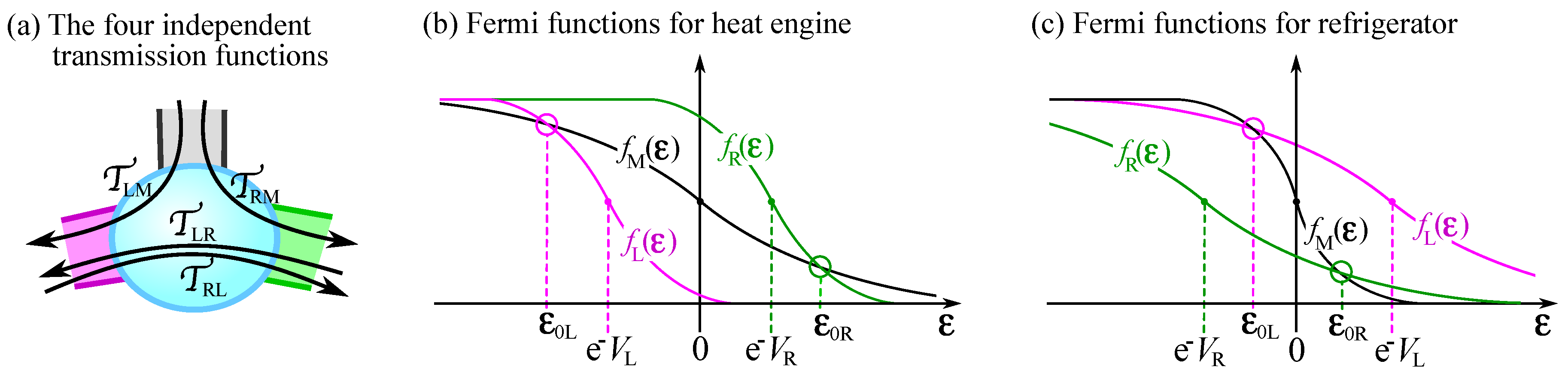
Our objective is to find the transmission functions, ${\mathcal{T}}_{\mathrm{LM}}\left(ϵ\right)$, ${\mathcal{T}}_{\mathrm{RM}}\left(ϵ\right)$, ${\mathcal{T}}_{\mathrm{LR}}\left(ϵ\right)$, and ${\mathcal{T}}_{\mathrm{RL}}\left(ϵ\right)$, that maximize the heat-engine efficiency for given power generation, $P_{\mathrm{gen}}$. This is equivalent to finding the transmission functions that minimize heat flow out of reservoir M, $J_{\mathrm{M}}$, for given $P_{\mathrm{gen}}$. To find these optimal transmission functions one must start with completely arbitrary ϵ dependences of the transmission functions. As in references [1,2], one can do this by considering each transmission function as consisting of an infinite number of slices, each of vanishing width δ. I define ${\tau }_{ij}^{\left(\gamma \right)}$ as the height of the γ-th slice of ${\mathcal{T}}_{ij}\left(ϵ\right)$, which is the slice with energy ${ϵ}_{\gamma }$. One then wants to optimize the biases of reservoirs L and R ($V_{\mathrm{L}}$ and $V_{\mathrm{R}}$) and each ${\tau }_{ij}^{\left(\gamma \right)}$; this requires finding the value of each of this infinite number of parameters that minimize $J_{\mathrm{M}}$ under the constraints that $I_{\mathrm{M}}=0$ and that $P_{\mathrm{gen}}$ is fixed at the value of interest.

The central ingredients in this optimization are the rate of change of $P_{\mathrm{gen}}$, $I_{\mathrm{M}}$ and $J_{\mathrm{M}}$ with ${\tau }_{ij}^{\left(\gamma \right)}$. Here,

$$\begin{array}{ccc}\frac{\mathrm{d}{P}_{\mathrm{gen}}}{\mathrm{d}{\tau }_{ij}^{\left(\gamma \right)}}{|}_{V,\tau }\hfill & =& e^{-}{V}_i\frac{\delta }{h}\left[f_j\left({ϵ}_{\gamma }\right)-f_i\left({ϵ}_{\gamma }\right)\right],\hfill \end{array}$$

(25)

where ${|}_{V,\tau }$ means the derivative is taken for fixed $V_{\mathrm{L}}$, $V_{\mathrm{R}}$ and fixed ${\tau }_{ij}^{\left({\gamma }^{\prime }\right)}$ for all ${\gamma }^{\prime }\ne \gamma$. Doing the same for $I_{\mathrm{M}}$ and $J_{\mathrm{M}}$, one gets for $ij\in \left\{\mathrm{LM},\mathrm{RM},\mathrm{LR},\mathrm{RL}\right\}$,

$$\begin{array}{ccc}\frac{\mathrm{d}{I}_{\mathrm{M}}}{\mathrm{d}{\tau }_{ij}^{\left(\gamma \right)}}{|}_{V,\tau }\hfill & =& \frac{1}{V_i}\frac{\mathrm{d}{P}_{\mathrm{gen}}}{\mathrm{d}{\tau }_{ij}^{\left(\gamma \right)}}{|}_{V,\tau },\hfill \end{array}$$

(26)

$$\begin{array}{ccc}\frac{\mathrm{d}{J}_{\mathrm{M}}}{\mathrm{d}{\tau }_{ij}^{\left(\gamma \right)}}{|}_{V,\tau }\hfill & =& \frac{{ϵ}_{\gamma }}{e^{-}{V}_i}\frac{\mathrm{d}{P}_{\mathrm{gen}}}{\mathrm{d}{\tau }_{ij}^{\left(\gamma \right)}}{|}_{V,\tau }.\hfill \end{array}$$

(27)

For a heat-engine, one considers the case where $T_{\mathrm{L}}=T_{\mathrm{R}}=T_0$ and $T_{\mathrm{M}}>T_0$, while $e^{-}{V}_{\mathrm{L}}<0<e^{-}{V}_{\mathrm{R}}$. The Fermi functions in this case are sketched in Figure 3a. One observes that

$$\begin{array}{ccc}\left[f_{\mathrm{R}}\left(ϵ\right)-f_{\mathrm{L}}\left(ϵ\right)\right]\hfill & \text{is}& \text{positive}\text{for}\text{all}ϵ,\hfill \end{array}$$

(28)

$$\begin{array}{ccc}\left[f_{\mathrm{M}}\left(ϵ\right)-f_i\left(ϵ\right)\right]\hfill & \text{is}& \left\{\begin{array}{c}\text{positive}\text{for}ϵ>{ϵ}_{0i},\hfill \\ \text{negative}\text{for}ϵ<{ϵ}_{0i},\hfill \end{array}\right.\hfill \end{array}$$

(29)

where we define

$$\begin{array}{c}{ϵ}_{0i}=\frac{e^{-}{V}_i}{1-T_0/T_{\mathrm{M}}}.\hfill \end{array}$$

(30)

We will take $V_{\mathrm{L}},V_{\mathrm{R}}$ such that $I_{\mathrm{M}}=0$, and

$$\begin{array}{c}{I}_{\mathrm{R}}=-I_{\mathrm{L}}>0.\hfill \end{array}$$

(31)

To proceed with the derivation, it is more convenient to assume that one is interested in minimizing the heat-flow $J_{\mathrm{M}}$ for given $P_{\mathrm{gen}}$ and given $I_{\mathrm{M}}$. Only at the end will we take $I_{\mathrm{M}}=0$ to arrive at the situation of interest.

3.1. Optimizing ${\mathcal{T}}_{\mathrm{RM}}$, ${\mathcal{T}}_{\mathrm{LM}}$, ${\mathcal{T}}_{\mathrm{RL}}$ and ${\mathcal{T}}_{\mathrm{LR}}$ Independently

One starts with the assumption that the four transmission functions, ${\mathcal{T}}_{\mathrm{RM}}$, ${\mathcal{T}}_{\mathrm{LM}}$, ${\mathcal{T}}_{\mathrm{RL}}$ and ${\mathcal{T}}_{\mathrm{LR}}$, each have a completely arbitrary energy dependence and can be optimized independently. Only in Section 3.2 do we take into account the relations between these transmission functions imposed by combining Equation (16) with Equation (19).

To carry out the independent optimization of each of the four transmission functions, let us define

$$\begin{array}{c}{\partial }_{\mathrm{R}}\cdots =\frac{\mathrm{d}(\cdots )}{\mathrm{d}{V}_{\mathrm{R}}}{|}_{V_{\mathrm{L}},\mathcal{T}},\text{and}{\partial }_{\mathrm{L}}\cdots =\frac{\mathrm{d}(\cdots )}{\mathrm{d}{V}_{\mathrm{L}}}{|}_{V_{\mathrm{R}},\mathcal{T}},\hfill \end{array}$$

(32)

where ${|}_{V_i,\mathcal{T}}$ indicates that the derivative is for fixed $V_i$ and fixed transmission functions. Then, for an inifinitesimal change of ${\tau }_{ij}^{\left(\gamma \right)}$, $V_{\mathrm{L}}$ and $V_{\mathrm{R}}$, one has:

$$\begin{array}{ccc}\delta J_{\mathrm{M}}\hfill & =& \frac{\mathrm{d}{J}_{\mathrm{M}}}{\mathrm{d}{\tau }_{ij}^{\left(\gamma \right)}}{|}_{V,\tau }\delta {\tau }_{ij}^{\left(\gamma \right)}+{\partial }_{\mathrm{L}}{J}_{\mathrm{M}}\delta V_{\mathrm{L}}+{\partial }_{\mathrm{R}}{J}_{\mathrm{M}}\delta V_{\mathrm{R}},\hfill \end{array}$$

(33)

$$\begin{array}{ccc}\delta I_{\mathrm{M}}\hfill & =& \frac{\mathrm{d}{I}_{\mathrm{M}}}{\mathrm{d}{\tau }_{ij}^{\left(\gamma \right)}}{|}_{V,\tau }\delta {\tau }_{ij}^{\left(\gamma \right)}+{\partial }_{\mathrm{L}}{I}_{\mathrm{M}}\delta V_{\mathrm{L}}+{\partial }_{\mathrm{R}}{I}_{\mathrm{M}}\delta V_{\mathrm{R}},\hfill \end{array}$$

(34)

$$\begin{array}{ccc}\delta P_{\mathrm{gen}}\hfill & =& \frac{\mathrm{d}{P}_{\mathrm{gen}}}{\mathrm{d}{\tau }_{ij}^{\left(\gamma \right)}}{|}_{V,\tau }\delta {\tau }_{ij}^{\left(\gamma \right)}+{\partial }_{\mathrm{L}}{P}_{\mathrm{gen}}\delta V_{\mathrm{L}}+{\partial }_{\mathrm{R}}{P}_{\mathrm{gen}}\delta V_{\mathrm{R}}.\hfill \end{array}$$

(35)

We are interested in fixed $P_{\mathrm{gen}}$ and $I_{\mathrm{M}}$, so we want $\delta I_{\mathrm{M}}=\delta P_{\mathrm{gen}}=0$. This means Equations (34) and (35) form a pair of simultaneous equations, which one solves to get

$$\begin{array}{ccc}\delta V_{\mathrm{L}}\hfill & =& \left[\frac{{\partial }_{\mathrm{R}}{I}_{\mathrm{M}}}{\mathcal{A}}\frac{\mathrm{d}{P}_{\mathrm{gen}}}{\mathrm{d}{\tau }_{ij}^{\left(\gamma \right)}}{|}_{V,\tau }-\frac{{\partial }_{\mathrm{R}}{P}_{\mathrm{gen}}}{\mathcal{A}}\frac{\mathrm{d}{I}_{\mathrm{M}}}{\mathrm{d}{\tau }_{ij}^{\left(\gamma \right)}}{|}_{V,\tau }\right]\delta {\tau }_{ij}^{\left(\gamma \right)},\hfill \\ \delta V_{\mathrm{R}}\hfill & =& \left[-\frac{{\partial }_{\mathrm{L}}{I}_{\mathrm{M}}}{\mathcal{A}}\frac{\mathrm{d}{P}_{\mathrm{gen}}}{\mathrm{d}{\tau }_{ij}^{\left(\gamma \right)}}{|}_{V,\tau }+\frac{{\partial }_{\mathrm{L}}{P}_{\mathrm{gen}}}{\mathcal{A}}\frac{\mathrm{d}{I}_{\mathrm{M}}}{\mathrm{d}{\tau }_{ij}^{\left(\gamma \right)}}{|}_{V,\tau }\right]\delta {\tau }_{ij}^{\left(\gamma \right)},\hfill \end{array}$$

where we define

$$\begin{array}{ccc}\mathcal{A}\hfill & =& {\partial }_{\mathrm{L}}{I}_{\mathrm{M}}{\partial }_{\mathrm{R}}{P}_{\mathrm{gen}}-{\partial }_{\mathrm{R}}{I}_{\mathrm{M}}{\partial }_{\mathrm{L}}{P}_{\mathrm{gen}}.\hfill \end{array}$$

We substitute these results for $\delta V_{\mathrm{L}}$ and $\delta V_{\mathrm{R}}$ into Equation (33) and use Equations (26) and (27) to cast everything in terms of $\mathrm{d}{P}_{\mathrm{gen}}/\mathrm{d}{\tau }_{ij}^{\left(\gamma \right)}$. Then, for $ij\in \left\{\mathrm{LM},\mathrm{RM},\mathrm{LR},\mathrm{RL}\right\}$,

$$\begin{array}{ccc}\delta J_{\mathrm{M}}\hfill & =& \delta {\tau }_{ij}^{\left(\gamma \right)}\left[\frac{{ϵ}_{\gamma }-{ϵ}_{1i}}{e^{-}{V}_i}\right]\frac{\mathrm{d}{P}_{\mathrm{gen}}}{\mathrm{d}{\tau }_{ij}^{\left(\gamma \right)}}{|}_{V,\tau },\hfill \end{array}$$

(36)

where we define ${ϵ}_{1i}$ with $i\in L,R$ as

$$\begin{array}{ccc}{ϵ}_{1i}\hfill & =& e^{-}{V}_i\frac{{\partial }_{\mathrm{R}}{J}_{\mathrm{M}}{\partial }_{\mathrm{L}}{I}_{\mathrm{M}}-{\partial }_{\mathrm{L}}{J}_{\mathrm{M}}{\partial }_{\mathrm{R}}{I}_{\mathrm{M}}}{\mathcal{A}}+e^{-}\frac{{\partial }_{\mathrm{L}}{J}_{\mathrm{M}}{\partial }_{\mathrm{R}}{P}_{\mathrm{gen}}-{\partial }_{\mathrm{R}}{J}_{\mathrm{M}}{\partial }_{\mathrm{L}}{P}_{\mathrm{gen}}}{\mathcal{A}}.\hfill \end{array}$$

(37)

Thus, using Equation (25), one can conclude that $J_{\mathrm{M}}$ shrinks upon increasing ${\tau }_{ij}^{\left(\gamma \right)}$ (for fixed $P_{\mathrm{gen}}$ and fixed $I_{\mathrm{M}}$) if

$$\begin{array}{ccc}\left[{ϵ}_{\gamma }-{ϵ}_{1i}\right]\left[f_j\left({ϵ}_{\gamma }\right)-f_i\left({ϵ}_{\gamma }\right)\right]\hfill & <& 0,\hfill \end{array}$$

(38)

and, otherwise, $J_{\mathrm{M}}$ grows upon increasing ${\tau }_{ij}^{\left(\gamma \right)}$. The sign of the difference of Fermi functions is given by Equations (28) and (29). Hence, $J_{\mathrm{M}}$ is reduced for fixed $P_{\mathrm{gen}}$ and fixed $I_{\mathrm{M}}$ by:

(a)

Increasing ${\mathcal{T}}_{\mathrm{RM}}\left(ϵ\right)$ up to $N_{\mathrm{RM}}^{\min }$ for ϵ between ${ϵ}_{0\mathrm{R}}$ and ${ϵ}_{1\mathrm{R}}$, while reducing ${\mathcal{T}}_{\mathrm{RM}}\left(ϵ\right)$ to zero for all other ϵ.

(b)

Increasing ${\mathcal{T}}_{\mathrm{LM}}\left(ϵ\right)$ up to $N_{\mathrm{LM}}^{\min }$ for ϵ between ${ϵ}_{0\mathrm{L}}$ and ${ϵ}_{1\mathrm{L}}$, while reducing ${\mathcal{T}}_{\mathrm{LM}}\left(ϵ\right)$ to zero for all other ϵ.

(c)

Increasing ${\mathcal{T}}_{\mathrm{RL}}\left(ϵ\right)$ up to $N_{\mathrm{RL}}^{\min }$ for $ϵ>{ϵ}_{1\mathrm{R}}$, while reducing ${\mathcal{T}}_{\mathrm{LM}}\left(ϵ\right)$ to zero for $ϵ<{ϵ}_{1\mathrm{R}}$.

(d)

Increasing ${\mathcal{T}}_{\mathrm{LR}}\left(ϵ\right)$ up to $N_{\mathrm{RL}}^{\min }$ for $ϵ<{ϵ}_{1\mathrm{L}}$, while reducing ${\mathcal{T}}_{\mathrm{LM}}\left(ϵ\right)$ to zero for $ϵ>{ϵ}_{1\mathrm{L}}$.

Here, it is Equation (16) that stops us from reducing these functions below zero, or increasing ${\mathcal{T}}_{ij}\left(ϵ\right)$ beyond $N_{ij}^{\min }$.

While it is hard to guess the form of ${ϵ}_{1\mathrm{L}}$ and ${ϵ}_{1\mathrm{R}}$ from their definition in Equation (37), by inspecting Equations (20) and (21), one sees that a heat-engine should have ${ϵ}_{1\mathrm{R}}>{ϵ}_{0\mathrm{R}}$ and ${ϵ}_{1\mathrm{L}}<{ϵ}_{0\mathrm{L}}$ to ensure that both terms contributing to $P_{\mathrm{gen}}$ in Equation (24) are positive. While refrigerators are not discussed until Section 7, it will shown there that their optimization leads to similar rules to (a)–(d) above. However, refrigerators must absorb electrical power (negative $P_{\mathrm{gen}}$), so they will have ${ϵ}_{1\mathrm{R}}<{ϵ}_{0\mathrm{R}}$ and ${ϵ}_{1\mathrm{L}}>{ϵ}_{0\mathrm{L}}$, with Section 7 also showing that ${ϵ}_{1\mathrm{R}}>0$ and ${ϵ}_{1\mathrm{L}}<0$. Thus, one will have to consider two situations,

$$\begin{array}{ccc}\text{heat-engine:}\hfill & & {ϵ}_{1\mathrm{L}}<{ϵ}_{0\mathrm{L}}<0<{ϵ}_{0\mathrm{R}}<{ϵ}_{1\mathrm{R}},\hfill \end{array}$$

(39a)

$$\begin{array}{ccc}\text{refrigerator:}\hfill & & {ϵ}_{0\mathrm{L}}<{ϵ}_{1\mathrm{L}}<0<{ϵ}_{1\mathrm{R}}<{ϵ}_{0\mathrm{R}},\hfill \end{array}$$

(39b)

as sketched in Figure 4a,b, respectively.

Problem with the Independent Optimization

The problem with the above solution is that it does not satisfy the constraints imposed by combining Equation (16) with Equation (19). Specifically, it does not satisfy the constraints

$$\begin{array}{ccc}0\hfill & \le & {\mathcal{T}}_{\mathrm{LM}}\left(ϵ\right)+{\mathcal{T}}_{\mathrm{LR}}\left(ϵ\right)-{\mathcal{T}}_{\mathrm{RL}}\left(ϵ\right)\le N_{\mathrm{ML}}^{\min },\hfill \end{array}$$

(40a)

$$\begin{array}{ccc}0\hfill & \le & {\mathcal{T}}_{\mathrm{RM}}\left(ϵ\right)+{\mathcal{T}}_{\mathrm{RL}}\left(ϵ\right)-{\mathcal{T}}_{\mathrm{LR}}\left(ϵ\right)\le N_{MR}^{\min }.\hfill \end{array}$$

(40b)

The proposed solution violates the lower bound in Equation (40a) for all $ϵ>{ϵ}_{1\mathrm{R}}$. Similarly, it violates the lower bound in Equation (40b) for all $ϵ<{ϵ}_{1\mathrm{L}}$. In addition, in the case of a refrigerator with ${ϵ}_{0\mathrm{R}}>{ϵ}_{1\mathrm{R}}$, as in Figure 4b, then the proposed solution violates the upper bound in Equation (40b) for all ${ϵ}_{1\mathrm{R}}<ϵ<{ϵ}_{0\mathrm{R}}$. Similarly, when ${ϵ}_{1\mathrm{L}}>{ϵ}_{0\mathrm{L}}$, the solution also violates the upper bound in Equation (40a) for all ${ϵ}_{0\mathrm{L}}<ϵ<{ϵ}_{1\mathrm{L}}$. I will fix this in the case of a heat-engine by explicitly adding these bounds in the next section, and the case of a refrigerator will be treated in Section 7.

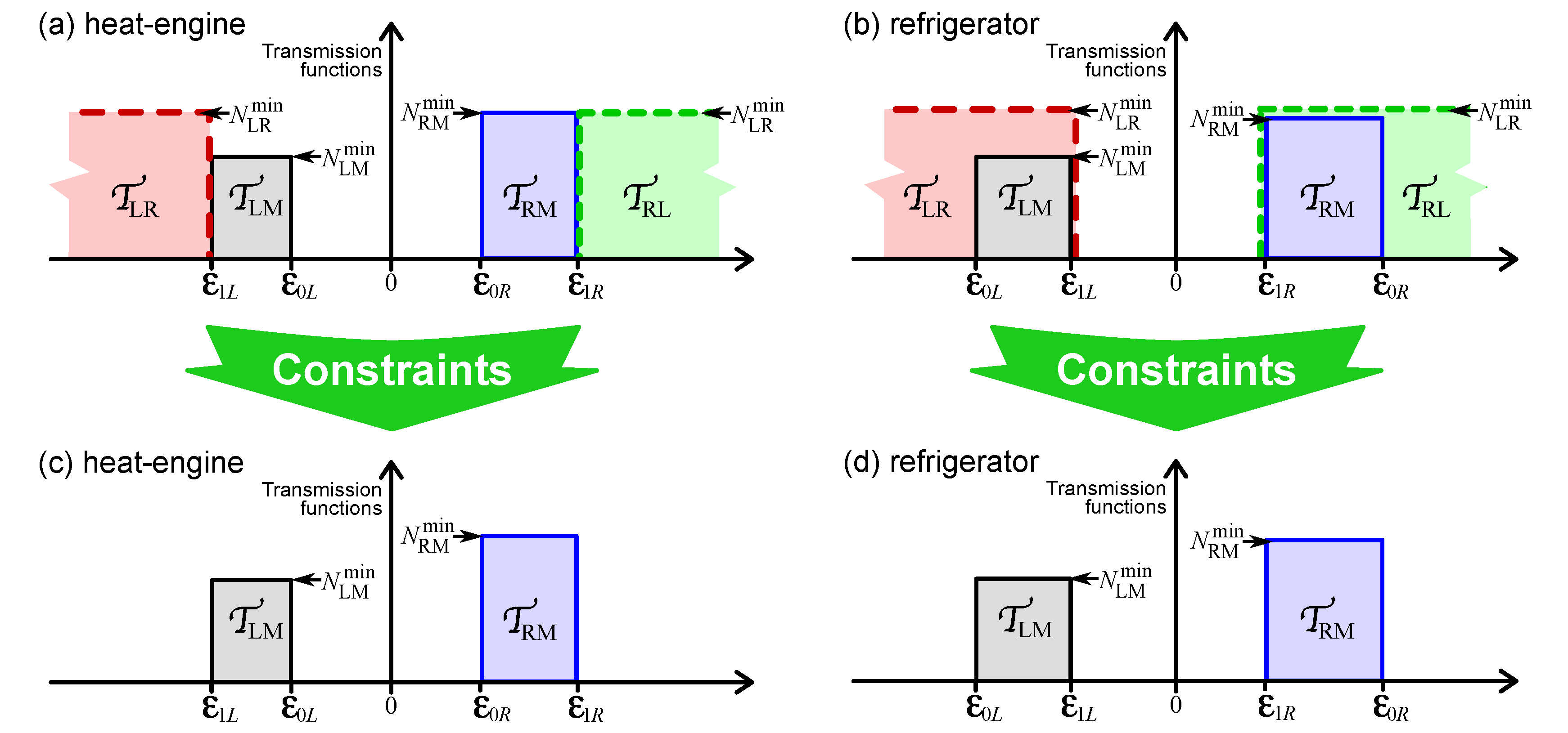
3.2. Optimizing Transmissions While Respecting All Constraints

Here, we consider carrying out the optimization given by the list (a)–(d) in the previous section within the limits given by the constraints in Equation (40). As we are considering a heat-engine, we know that the ${ϵ}_{0\mathrm{L}}$, ${ϵ}_{1\mathrm{L}}$, ${ϵ}_{0\mathrm{R}}$ and ${ϵ}_{1\mathrm{R}}$ are ordered as in Equation (39a) (see Figure 4a). The optimization for ϵ in the window between ${ϵ}_{1\mathrm{L}}$ and ${ϵ}_{1\mathrm{R}}$ is trivial, since there the transmission functions in the above list (a–d) do not violate the constraints in Equation (16). This leaves us with the less trivial part of the optimization under the constraints, for $ϵ>{ϵ}_{1\mathrm{R}}$ and $ϵ<{ϵ}_{1\mathrm{L}}$.

3.2.1. Optimization for $ϵ>{ϵ}_{1\mathrm{R}}$ or $ϵ<{ϵ}_{1\mathrm{L}}$

For $ϵ>{ϵ}_{1\mathrm{R}}$, the independent optimization of the transmission functions required increasing ${\mathcal{T}}_{\mathrm{RL}}$ while decreasing ${\mathcal{T}}_{\mathrm{LM}}$ and ${\mathcal{T}}_{\mathrm{LR}}$ but doing this comes into conflict with the constraint that ${\mathcal{T}}_{\mathrm{LR}}\ge {\mathcal{T}}_{\mathrm{RL}}-{\mathcal{T}}_{\mathrm{LM}}$ due to Equation (40a). Thus, one can do the unconstrained optimization in the previous section up to the point allowed by the constraint, after which

$$\begin{array}{c}{\mathcal{T}}_{\mathrm{LR}}\left(ϵ\right)={\mathcal{T}}_{\mathrm{RL}}\left(ϵ\right)-{\mathcal{T}}_{\mathrm{LM}}\left(ϵ\right).\hfill \end{array}$$

(41)

We then ask if $J_{\mathrm{M}}$ decreases (for fixed power generation) when we increase slice γ of ${\mathcal{T}}_{\mathrm{RL}}$ and ${\mathcal{T}}_{\mathrm{LM}}$ by infinitesimal amounts $\delta {\tau }_{\mathrm{RL}}^{\left(\gamma \right)}$ and $\delta {\tau }_{\mathrm{LM}}^{\left(\gamma \right)}$, respectively, given that one must also change slice γ of ${\mathcal{T}}_{\mathrm{LR}}$ by $\delta {\tau }_{\mathrm{LR}}^{\left(\gamma \right)}=\delta {\tau }_{\mathrm{RL}}^{\left(\gamma \right)}-\delta {\tau }_{\mathrm{LM}}^{\left(\gamma \right)}$ not to violate the above constraint. With this observation, we find that, for $J_{\mathrm{M}}$ to decrease, we need:

$$\begin{array}{ccc}& & \delta {\tau }_{\mathrm{RL}}^{\left(\gamma \right)}({ϵ}_{1\mathrm{R}}-{ϵ}_{1\mathrm{L}})\left[f_{\mathrm{R}}\left({ϵ}_{\gamma }\right)-f_{\mathrm{L}}\left({ϵ}_{\gamma }\right)\right]+\delta {\tau }_{\mathrm{LM}}^{\left(\gamma \right)}({ϵ}_{\gamma }-{ϵ}_{1\mathrm{L}})\left[f_{\mathrm{M}}\left({ϵ}_{\gamma }\right)-f_{\mathrm{R}}\left({ϵ}_{\gamma }\right)\right]<0.\hfill \end{array}$$

(42)

Since all the brackets in the above expression are positive for ${ϵ}_{\gamma }>{ϵ}_{0\mathrm{R}}$, we see that to minimize $J_{\mathrm{M}}$, we should minimize both ${\mathcal{T}}_{\mathrm{RL}}$ and ${\mathcal{T}}_{\mathrm{LM}}$. Thus, we conclude that, for $ϵ>{ϵ}_{1\mathrm{R}}$, it is optimal that all transmission functions are zero.

The situation where $ϵ<{ϵ}_{1\mathrm{L}}$ can be treated in the same manner as above, upon interchanging the labels “L” and “R”. Thus, the optimal situation is when all transmission functions are zero for $ϵ<{ϵ}_{1\mathrm{L}}$.

3.2.2. Conclusion of Optimization with Constraints

Bringing together the results found so far, the transmission functions which maximize the heat-engine’s efficiency for a given power generation are:

$$\begin{array}{ccc}{\mathcal{T}}_{\mathrm{RL}}\left(ϵ\right)={\mathcal{T}}_{\mathrm{LR}}\left(ϵ\right)=0\text{for}\text{all}ϵ,\hfill & & \hfill \end{array}$$

(43a)

$$\begin{array}{ccc}{\mathcal{T}}_{\mathrm{RM}}\left(ϵ\right)=\left\{\begin{array}{ccc}{N}_{\mathrm{RM}}^{\min }& & \text{for}{ϵ}_{0\mathrm{R}}\le ϵ\le {ϵ}_{1\mathrm{R}}\hfill \\ 0& & \text{otherwise}\hfill \end{array},\right.\hfill & & \end{array}$$

(43b)

$$\begin{array}{ccc}{\mathcal{T}}_{\mathrm{LM}}\left(ϵ\right)=\left\{\begin{array}{ccc}{N}_{\mathrm{LM}}^{\min }& & \text{for}{ϵ}_{1\mathrm{L}}\le ϵ\le {ϵ}_{0\mathrm{L}}\hfill \\ 0& & \text{otherwise}\hfill \end{array},\right.\hfill & & \hfill \end{array}$$

(43c)

where $N_{ij}^{\min }$ is defined in Equation (17). These functions are sketched in Figure 4c. Equation (43a) means the optimal system has no direct flow of electrons between reservoirs L and R. Given Equations (19d) and (19e), this means that

$$\begin{array}{c}{\mathcal{T}}_{\mathrm{MR}}\left(ϵ\right)={\mathcal{T}}_{\mathrm{RM}}\left(ϵ\right)\&{\mathcal{T}}_{\mathrm{ML}}\left(ϵ\right)={\mathcal{T}}_{\mathrm{LM}}\left(ϵ\right)\text{for}\text{all}ϵ.\hfill \end{array}$$

(43d)

Hence, the optimal three-terminal situation is one that can be thought of as a pair of two-terminal problems much like those already considered in references [1,2]. To be more explicit, Equation (43) tells us that the optimal transmission is one that can be split into a problem of optimizing transmission between M and R through $N_{\mathrm{RM}}^{\min }$ transverse modes (with ${\mathcal{T}}_{\mathrm{MR}}\left(ϵ\right)={\mathcal{T}}_{\mathrm{RM}}\left(ϵ\right)$ at all ϵ) and another problem of optimizing transmission between M and L through $N_{\mathrm{LM}}^{\min }$ transverse modes (with ${\mathcal{T}}_{\mathrm{ML}}\left(ϵ\right)={\mathcal{T}}_{\mathrm{LM}}\left(ϵ\right)$ at all ϵ). These two optimization problems could be treated independently were it not for the fact they are coupled by the constraint that the electrical currents in the two problems $I_{\mathrm{L}}$ and $I_{\mathrm{R}}$ must sum to zero to get Equation (1).

4. Showing the Three-Terminal System Cannot Exceed the Bound for Two-Terminal Systems

Given the previous section’s observation that the optimal transmission for a three-terminal system is one that can be split into a pair of two-terminal transmission problems, two conclusions can be drawn.

Firstly, the optimal transmission for a three-terminal system does not require any time-reversal symmetry breaking of the type generated by an external magnetic field. Thus, the optimal transmission can be achieved in a system without an external magnetic field. I wish to be clear that this proof does not mean that magnetic fields may not be helpful in specific situations; for example, a magnetic field may be helpful in tuning the transmission of a given system to be closer to the optimal one. However, it does mean that there is no requirement to have a magnetic field; other parameters (which do not break time-reversal symmetry) can be tuned to bring the system’s transmission to the optimal one. This is the first main conclusion of this work.

Secondly, it is not hard to show that a three-terminal system cannot exceed the bounds found in references [1,2] for a pair of two-terminal systems with the same number of transverse modes. To be more specific, it cannot exceed the bound for a pair of two-terminal systems where one of the two-terminal systems has $N_{\mathrm{LM}}^{\min }$ transverse modes and the other has $N_{\mathrm{RM}}^{\min }$ transverse modes (see Equation (17)). To prove this bound, it is sufficient to remark that the optimization of the three-terminal system in Equation (43) is exactly that of the optimization of a pair of two-terminal systems, with an additional constraint that the electrical currents in the two problems ($I_{\mathrm{L}}$ and $I_{\mathrm{R}}$) sum to zero. This constraint couples the two problems and makes them much harder to resolve. However, if we simply drop the constraint on $I_{\mathrm{L}}$ and $I_{\mathrm{R}}$ and perform the optimization, we can be certain that we are overestimating the efficiency at given power output. Once we drop this constraint, the two optimization problems become completely decoupled from each other. Thus, we can optimize the transmission between M and R using the method in references [1,2], and independently optimize the transmission between M and L using the same method. As a result, an overestimate of the three-terminal efficiency at given power output is bounded by the maximum two-terminal efficiency of a pair of two-terminal systems, with this bound being the one found in references [1,2]. This is the second main conclusion of this work.

5. Achieving the Two-Terminal Bound in a Three-Terminal System

Having found an upper bound on the efficiency at given power output by using a process that overestimates the efficiency, one can be sure that no three-terminal system can be more efficient than a pair of optimal two-terminal systems. This makes it natural to ask if any three-terminal system can be as efficient as this pair of optimal two-terminal systems. To answer this question, I present an example of a three-terminal system which is as efficient as the pair of optimal two-terminal systems. This will be our proof that the upper bound on the efficiency of a three-terminal system coincides with the upper bound on the efficiency of a pair of two-terminal systems.

To proceed, I take a three-terminal system with $N_{\mathrm{LM}}^{\min }=N_{\mathrm{RM}}^{\min }$. Given Equation (17), this could be a system with $N_{\mathrm{L}}=N_{\mathrm{R}}$, or it could be a system with $N_{\mathrm{M}}$ less than both $N_{\mathrm{L}}$ and $N_{\mathrm{R}}$, In this case, one can take a pair of optimal two-terminal solutions from refrences [1,2], in the cases where $e^{-}{V}_{\mathrm{R}}=-e^{-}{V}_{\mathrm{L}}>0$. They have

$$\begin{array}{c}{ϵ}_{0\mathrm{L}}=-{ϵ}_{0\mathrm{R}}\&{ϵ}_{1\mathrm{L}}=-{ϵ}_{1\mathrm{R}},\hfill \end{array}$$

(44a)

with

$$\begin{array}{c}{ϵ}_{0\mathrm{R}}=\frac{e^{-}{V}_R}{1-T_{\mathrm{R}}/T_{\mathrm{M}}}\&{ϵ}_{1\mathrm{R}}=e^{-}{V}_R\frac{{\partial }_{\mathrm{R}}{J}_M^{\left(\mathrm{R}\right)}}{{\partial }_{\mathrm{R}}{P}_{\mathrm{gen}}^{\left(\mathrm{R}\right)}},\hfill \end{array}$$

(44b)

where I have written the results of references [1,2] in terms of the notation of this article, with the derivatives defined in Equation (32). Here, $J_M^{\left(i\right)}$ is the part of the heat carried out of reservoir M by electron flow between reservoir M and reservoir i, and $P_{\mathrm{gen}}^{\left(i\right)}$ is the part of the total power generated by that electron flow, so

$$\begin{array}{ccc}{J}_{\mathrm{M}}\hfill & =& J_{\mathrm{M}}^{\left(\mathrm{R}\right)}+J_{\mathrm{M}}^{\left(\mathrm{L}\right)},\hfill \end{array}$$

(45a)

$$\begin{array}{ccc}{P}_{\mathrm{gen}}\hfill & =& P_{\mathrm{gen}}^{\left(\mathrm{R}\right)}+P_{\mathrm{gen}}^{\left(\mathrm{L}\right)}.\hfill \end{array}$$

(45b)

Conservation of electrical current gives $I_{\mathrm{M}}=-I_{\mathrm{L}}-I_{\mathrm{R}}$. As the only dependence on $V_i$ within $I_{\mathrm{M}}$, $J_{\mathrm{M}}$ and $P_{\mathrm{gen}}$ are in $I_i$, $J_{\mathrm{M}}^{\left(i\right)}$ and $P_{\mathrm{gen}}^{\left(i\right)}$, respectively, and one has

$$\begin{array}{c}{\partial }_{\mathrm{i}}{I}_{\mathrm{M}}=-{\partial }_{\mathrm{i}}{I}_{\mathrm{i}},{\partial }_{\mathrm{i}}{J}_{\mathrm{M}}={\partial }_{\mathrm{i}}{J}_{\mathrm{M}}^{\left(i\right)}\text{and}{\partial }_{\mathrm{i}}{P}_{\mathrm{gen}}={\partial }_{\mathrm{i}}{P}_{\mathrm{gen}}^{\left(i\right)}.\hfill \end{array}$$

(46)

With some thought about the symmetries between L and R, one sees that the derivatives have the following symmetries between L and R,

$$\begin{array}{ccc}{\partial }_{\mathrm{L}}{I}_{\mathrm{M}}\hfill & =& {\partial }_{\mathrm{R}}{I}_{\mathrm{M}},\hfill \end{array}$$

(47a)

$$\begin{array}{ccc}{\partial }_{\mathrm{L}}{J}_{\mathrm{M}}\hfill & =& -{\partial }_{\mathrm{R}}{J}_{\mathrm{M}},\hfill \end{array}$$

(47b)

$$\begin{array}{ccc}{\partial }_{\mathrm{L}}{P}_{\mathrm{gen}}\hfill & =& -{\partial }_{\mathrm{R}}{P}_{\mathrm{gen}}.\hfill \end{array}$$

(47c)

We recall that Equations (44)–(47) are all for an optimal pair of two-terminal systems. We now take the information in Equations (44)–(47), and verify that they also give an optimal solution of the three-terminal problem. For this, we note that the definition of ${ϵ}_{0\mathrm{R}}$ and ${ϵ}_{0\mathrm{L}}$ are the same in the two- and three-terminal problems; however, the definition of ${ϵ}_{1\mathrm{R}}$ and ${ϵ}_{1\mathrm{L}}$ are different, with that for three-terminals being Equation (37) and that for two-terminals being Equation (44b). However, if we now take the symmetry relations in Equation (47), we see that Equation (37) reduces to Equation (44b). Thus, the solution of the optimization problem for a pair of two-terminal systems in Equations (44)–(47) is also a solution of the optimization problem for the three-terminal problem. All currents are the same in the three-terminal system as in the pair of two-terminal systems, so the efficiency and power output are also the same. Finally, we note that this solution has $I_{\mathrm{L}}=-I_{\mathrm{R}}$, so it satisfies $I_{\mathrm{M}}=0$ as in Equation (1). Hence, we have shown that an optimal three-terminal system can be as good as a pair of optimal two-terminal systems. This is the third main conclusion of this work (after the two in the previous section).

Combining this conclusion with the others, one finds that the upper bound on efficiency at a given power output is the same for a three-terminal system as for a pair of two terminal systems. This means that the optimal three-terminal system has no advantage over a pair of optimal two-terminal systems; however, it does not tell us in which geometry it is easier to engineer a system that achieves (or gets close to) that optimum.

6. Route to the Optimal Transmission for $N_{\mathrm{LM}}^{\min }\ne N_{\mathrm{RM}}^{\min }$

One can use the results of the two preceding sections to get a simple over-estimate of the maximal efficiency at given power generation for a machine with $N_{\mathrm{LM}}^{\min }\ne N_{\mathrm{RM}}^{\min }$. This upper bound is given by the efficiency of an equivalent three-terminal machine with $N_{\mathrm{LM}}^{\min }=N_{\mathrm{RM}}^{\min }$. Here, I define an “equivalent” system as one with the same $N_{\mathrm{LM}}^{\min }+N_{\mathrm{RM}}^{\min }$. In the case where $N_{\mathrm{M}}>N_{\mathrm{L}},N_{\mathrm{R}}$, this is the same as saying that, for given $N_{\mathrm{L}}+N_{\mathrm{R}}$, an optimal machine with $N_{\mathrm{L}}\ne N_{\mathrm{R}}$ cannot be better than an optimal machine with $N_{\mathrm{L}}=N_{\mathrm{R}}$. While for $N_{\mathrm{M}}<N_{\mathrm{L}},N_{\mathrm{R}}$, all systems have $N_{\mathrm{LM}}^{\min }=N_{\mathrm{RM}}^{\min }$. However, it is likely that this upper bound for $N_{\mathrm{LM}}^{\min }\ne N_{\mathrm{RM}}^{\min }$ is clearly an overestimate, since it is probably only for $N_{\mathrm{LM}}^{\min }=N_{\mathrm{RM}}^{\min }$ that the optimal efficiency with the constraint that $I_{\mathrm{M}}=0$ is as large as that without this constraint. This greatly reduces practical interest in optimizing a system with $N_{\mathrm{LM}}^{\min }\ne N_{\mathrm{RM}}^{\min }$, since optimizing implies a significant amount of control over the system, in which case it is better to engineer the system to have $N_{\mathrm{LM}}^{\min }=N_{\mathrm{RM}}^{\min }$, and optimize this.

If one wished, one could get a strict upper-bound on efficiency at given power generation for a system with given $N_{\mathrm{LM}}^{\min }\ne N_{\mathrm{RM}}^{\min }$. However, the optimization procedure for this is heavy, as well of being of little practical interest. Thus, I do not carry it out here, I simply list the principle steps.

(i)

Write explicit results for the currents and power in terms of four parameters ${ϵ}_{1\mathrm{L}}$, ${ϵ}_{1\mathrm{R}}$, $V_{\mathrm{L}}$ and $V_{\mathrm{R}}$ (noting that ${ϵ}_{0\mathrm{L}}$ and ${ϵ}_{0\mathrm{R}}$ are given by $V_{\mathrm{L}}$ and $V_{\mathrm{R}}$ in Equation (30)). Use these to calculate the derivatives that appear on the right-hand side of Equation (37), getting them as explicit functions of ${ϵ}_{1\mathrm{L}}$, ${ϵ}_{1\mathrm{R}}$, $V_{\mathrm{L}}$ and $V_{\mathrm{LR}}$. This step is straight-forward and is carried out in Appendix A.

(ii)

Substitute these derivatives into the right hand side of Equation (37) for $i=\mathrm{L}$ and $i=\mathrm{R}$, and this gives a pair of transcendental equations for the four parameters ${ϵ}_{1\mathrm{L}}$, ${ϵ}_{1\mathrm{R}}$, $V_{\mathrm{L}}$ and $V_{\mathrm{R}}$. Since one is interested in $I_{\mathrm{L}}=-I_{\mathrm{R}}$, with $I_{\mathrm{L}}$ and $I_{\mathrm{R}}$ being algebraic functions calculated in step (i) above (see Appendix A), this gives a third transcendental equation for these four parameters.

(iii)

Solve the three simultaneous transcendental equations numerically. As one has four unknown parameters and only three equations, we will get three parameters in terms of the fourth. I propose getting ${ϵ}_{1\mathrm{L}}$, ${ϵ}_{1\mathrm{R}}$, and $V_{\mathrm{L}}$ as functions of $V_{\mathrm{R}}$. This involves solving the set of three simultaneous equations once for each value of $V_{\mathrm{R}}$. This is the heavy part of the calculation, which one would have to perform numerically. I do not do this here.

(iv)

Once one has ${ϵ}_{1\mathrm{L}}$, ${ϵ}_{1\mathrm{R}}$, and $V_{\mathrm{L}}$ as a function of $V_{\mathrm{R}}$, one can get all electrical and heat currents as a function of $V_{\mathrm{R}}$ alone. Since step (iii) was performed numerically, we are forced to do this step numerically as well. The electrical currents give us the power generated, $P_{\mathrm{gen}}$, as a function of the voltage $V_{\mathrm{R}}$, which one must invert (again numerically) to get the voltage as a function of the power generated, $V_{\mathrm{R}}\left(P_{\mathrm{gen}}\right)$. One then takes the result for $J_{\mathrm{M}}$ as a function of $V_{\mathrm{R}}$ and substitute in $V_{\mathrm{R}}\left(P_{\mathrm{gen}}\right)$. This will give us $J_{\mathrm{M}}\left(P_{\mathrm{gen}}\right)$, the optimal (minimum) heat flow out of reservoir M for a given power generated. Then, the maximal heat-engine efficiency ${\eta }_{\mathrm{eng}}\left(P_{\mathrm{gen}}\right)=P_{\mathrm{gen}}/J_{\mathrm{M}}\left(P_{\mathrm{gen}}\right)$.

7. Maximum Refrigerator Efficiency for Given Cooling Power

In references [1,2], an upper bound on refrigerator efficiency for given cooling power was calculated directly for two-terminal devices. The result looked extremely similar to those works’ results for the upper bound on heat-engine efficiency for given power output. It has since become clear to us how to get the result for refrigerators from the result for heat-engines. The trick it to make the physically plausible assumption that the upper bound on the cooling power of a refrigerator, $J_{\mathrm{M}}$, is a monotonic function of the electrical power it absorbs, $P_{\mathrm{abs}}$. Then, the curve of maximum efficiency versus cooling power, $J_{\mathrm{M}}$, is the same as the curve of maximum efficiency versus absorbed power $P_{\mathrm{abs}}$ (upon transforming the horizontal axis from $P_{\mathrm{abs}}$ to $J_{\mathrm{M}}$ using the maximal efficiency curve). This is a great simplification of the problem, as it turns out that finding the refrigerator with maximal efficiency at given absorbed power is a rather straightforward extension of the above calculation of the optimal heat-engine at given power output.

Here, I take this point of view and find the three-terminal refrigerator with maximal efficiency for given absorbed power by a few straightforward modifications of the heat-engine calculation. A system absorbing power $P_{\mathrm{abs}}$ is the same as a system generating negative power $P_{\mathrm{gen}}=-P_{\mathrm{abs}}$. The crucial modification is that one must maximize $J_{\mathrm{M}}$ at given negative $P_{\mathrm{gen}}$ for refrigerators, when one was minimizing $J_{\mathrm{M}}$ at given positive $P_{\mathrm{gen}}$ for heat-engines.

Inspecting the calculation in Section 3, one sees that everything follows through for a refrigerator with $T_{\mathrm{L}}=T_{\mathrm{R}}=T_0$, $T_{\mathrm{M}}<T_0$, and $e^{-}{V}_{\mathrm{L}}>0>e^{-}{V}_{\mathrm{R}}$. Except that now, one is maximizing $J_{\mathrm{M}}$, and that now the Fermi functions in this case are those sketched in Figure 3b, obeying:

$$\begin{array}{ccc}\left[f_{\mathrm{R}}\left(ϵ\right)-f_{\mathrm{L}}\left(ϵ\right)\right]\hfill & \text{is}& \text{negative}\text{for}\text{all}ϵ,\hfill \end{array}$$

(48)

$$\begin{array}{ccc}\left[f_{\mathrm{M}}\left(ϵ\right)-f_i\left(ϵ\right)\right]\hfill & \text{is}& \left\{\begin{array}{c}\text{negative}\text{for}ϵ>{ϵ}_{0i}\hfill \\ \text{positive}\text{for}ϵ<{ϵ}_{0i}\hfill \end{array},\right.\hfill \end{array}$$

(49)

where Equation (30) is more conveniently written as

$$\begin{array}{c}{ϵ}_{0i}=\frac{-e^{-}{V}_i}{T_0/T_{\mathrm{M}}-1}.\hfill \end{array}$$

(50)

By a careful comparison with Section 3, one notes that all relevant differences of Fermi functions in the refrigerator case have the opposite sign from in the heat-engine case. Thus, if a given change of transmission reduces $J_{\mathrm{M}}$ for the heat-engine, then that same change will increase $J_{\mathrm{M}}$ for the refrigerator. Hence, one can conclude that the procedure that optimizes a heat-engine (minimizing $J_{\mathrm{M}}$ for given $P_{\mathrm{gen}}$ and $I_{\mathrm{M}}$) also optimizes a refrigerator (maximizing $J_{\mathrm{M}}$ for given $P_{\mathrm{gen}}$ and $I_{\mathrm{M}}$).

The independent optimization of ${\mathcal{T}}_{\mathrm{RM}}$, ${\mathcal{T}}_{\mathrm{LM}}$, ${\mathcal{T}}_{\mathrm{RL}}$ and ${\mathcal{T}}_{\mathrm{LR}}$ follows exactly as in Section 3.1. As with the heat-engine, it is difficult to guess the values of ${ϵ}_{1\mathrm{R}}$ and ${ϵ}_{1\mathrm{L}}$ from their definition in Equation (37). However, for maximal refrigeration, one wants both terms in $P_{\mathrm{gen}}$ in Equation (24) to be negative (so the absorbed power $P_{\mathrm{abs}}=-P_{\mathrm{gen}}>0$). By inspection of Equations (20) and (21), we see that this requires ${ϵ}_{1\mathrm{R}}<{ϵ}_{0\mathrm{R}}$ and ${ϵ}_{1\mathrm{L}}>{ϵ}_{0\mathrm{L}}$. Furthermore, one can see that ${ϵ}_{1\mathrm{L}}$ must be negative. To do this, one should inspect the terms in Equations (23) and (24) which depend on ${ϵ}_{1\mathrm{L}}$. Making ${ϵ}_{1\mathrm{L}}$ positive will increase $P_{\mathrm{abs}}$, while reducing the cooling power $J_{\mathrm{M}}$, which is clearly not a way to maximize the efficiency, ${\eta }_{\mathrm{fri}}$. A similar argument convinces us that ${ϵ}_{1\mathrm{R}}$ must be positive. Thus, we are interested in the case summarized in Equation (39b).

7.1. Optimizing Refrigerator While Respecting All Constraints

As we have ${ϵ}_{0\mathrm{L}}<{ϵ}_{1\mathrm{L}}<0<{ϵ}_{1\mathrm{R}}<{ϵ}_{0\mathrm{R}}$, the result of independently optimizing the transmission functions is that shown in Figure 4b. For ϵ between ${ϵ}_{1\mathrm{L}}$ and ${ϵ}_{1\mathrm{R}}$, no constraints are violated by that result; thus, the optimal solution remains that all transmission functions are zero in this window. The optimization for $ϵ>{ϵ}_{0\mathrm{R}}$ and $ϵ<{ϵ}_{0\mathrm{L}}$ follows the same logic as in Section 3.2.1, except that now one wants to maximize $J_{\mathrm{M}}$, and the differences of Fermi functions have the opposite signs. One finds that the system is optimized by having all transmission functions equal to zero for $ϵ>{ϵ}_{0\mathrm{R}}$ and for $ϵ<{ϵ}_{0\mathrm{L}}$.

7.1.1. Optimization for ϵ between ${ϵ}_{0\mathrm{R}}$ and ${ϵ}_{1\mathrm{R}}$.

For ϵ in the window ${ϵ}_{1\mathrm{R}}<ϵ<{ϵ}_{0\mathrm{R}}$, the independent optimization (maximizing ${\mathcal{T}}_{\mathrm{RM}}$ and ${\mathcal{T}}_{\mathrm{RL}}$, while minimizing all other transmissions) violates both the lower bound in Equation (40a) and the upper bound in Equation (40b). This case must be treated with care. We start by increasing ${\mathcal{T}}_{\mathrm{RM}}$ and ${\mathcal{T}}_{\mathrm{RL}}$ while reducing ${\mathcal{T}}_{\mathrm{LM}}$ and ${\mathcal{T}}_{\mathrm{LR}}$, until we reach the limit of the bounds in Equations (40a) and (40b); this occurs at

$$\begin{array}{ccc}{\mathcal{T}}_{\mathrm{LM}}\left(ϵ\right)\hfill & =& {\mathcal{T}}_{\mathrm{RL}}\left(ϵ\right)-{\mathcal{T}}_{\mathrm{LR}}\left(ϵ\right),\hfill \end{array}$$

(51)

$$\begin{array}{ccc}{\mathcal{T}}_{\mathrm{RM}}\left(ϵ\right)\hfill & =& -{\mathcal{T}}_{\mathrm{RL}}\left(ϵ\right)+{\mathcal{T}}_{\mathrm{LR}}\left(ϵ\right)+N_{\mathrm{MR}}^{\min }\left(ϵ\right).\hfill \end{array}$$

(52)

We then ask if $J_{\mathrm{M}}$ increases (for fixed $P_{\mathrm{abs}}$) when we increase slice γ of ${\mathcal{T}}_{\mathrm{RL}}$ and ${\mathcal{T}}_{\mathrm{LR}}$ by infinitesimal amounts $\delta {\tau }_{\mathrm{RL}}^{\left(\gamma \right)}$ and $\delta {\tau }_{\mathrm{LR}}^{\left(\gamma \right)}$, respectively, given that the above constraint means that one must also change slice γ of ${\mathcal{T}}_{\mathrm{LM}}$ by $\delta {\tau }_{\mathrm{LM}}^{\left(\gamma \right)}=\delta {\tau }_{\mathrm{RL}}^{\left(\gamma \right)}-\delta {\tau }_{\mathrm{LM}}^{\left(\gamma \right)}$, and change slice γ of ${\mathcal{T}}_{\mathrm{RM}}$ by $\delta {\tau }_{\mathrm{LM}}^{\left(\gamma \right)}=-\delta {\tau }_{\mathrm{RL}}^{\left(\gamma \right)}+\delta {\tau }_{\mathrm{LM}}^{\left(\gamma \right)}$. With this observation, we find that, for $J_{\mathrm{M}}$ to increase, we need:

$$\begin{array}{ccc}& & \delta {\tau }_{\mathrm{RL}}^{\left(\gamma \right)}({ϵ}_{1\mathrm{R}}-{ϵ}_{1\mathrm{L}})\left[f_{\mathrm{M}}\left({ϵ}_{\gamma }\right)-f_{\mathrm{L}}\left({ϵ}_{\gamma }\right)\right]+\delta {\tau }_{\mathrm{LR}}^{\left(\gamma \right)}({ϵ}_{1\mathrm{R}}-{ϵ}_{1\mathrm{L}})\left[f_{\mathrm{R}}\left({ϵ}_{\gamma }\right)-f_{\mathrm{M}}\left({ϵ}_{\gamma }\right)\right]>0.\hfill \end{array}$$

(53)

Since all brackets in the above expression are negative for ${ϵ}_{\gamma }<{ϵ}_{0\mathrm{R}}$, we see that to maximize $J_{\mathrm{M}}$, we should minimize both ${\mathcal{T}}_{\mathrm{RL}}$ and ${\mathcal{T}}_{\mathrm{LR}}$. Thus, the optimum for ϵ between ${ϵ}_{1\mathrm{R}}$ and ${ϵ}_{0\mathrm{R}}$ is that ${\mathcal{T}}_{\mathrm{RM}}$ is maximal (${\mathcal{T}}_{\mathrm{RM}}=N_{\mathrm{RM}}^{\min }$) while the other transmission functions are zero.

The same logic can be applied to the energies ϵ between ${ϵ}_{0\mathrm{L}}$ and ${ϵ}_{1\mathrm{L}}$, and we conclude that the optimal there is that ${\mathcal{T}}_{\mathrm{LM}}$ is maximal (${\mathcal{T}}_{\mathrm{LM}}=N_{\mathrm{LM}}^{\min }$) while the other transmission functions are zero.

7.1.2. Conclusion of Optimization with Constraints

To summarize, the transmission functions which maximize refrigerator cooling power $J_{\mathrm{M}}$ for given absorbed power $P_{\mathrm{abs}}$ are:

$$\begin{array}{ccc}{\mathcal{T}}_{\mathrm{RL}}\left(ϵ\right)={\mathcal{T}}_{\mathrm{LR}}\left(ϵ\right)=0\text{for}\text{all}ϵ,\hfill & & \end{array}$$

(54a)

$$\begin{array}{ccc}{\mathcal{T}}_{\mathrm{RM}}\left(ϵ\right)=\left\{\begin{array}{ccc}{N}_{\mathrm{RM}}^{\min }& & \text{for}{ϵ}_{1\mathrm{R}}\le ϵ\le {ϵ}_{0\mathrm{R}}\hfill \\ 0& & \text{otherwise}\hfill \end{array},\right.\hfill & & \end{array}$$

(54b)

$$\begin{array}{ccc}{\mathcal{T}}_{\mathrm{LM}}\left(ϵ\right)=\left\{\begin{array}{ccc}{N}_{\mathrm{LM}}^{\min }& & \text{for}{ϵ}_{0\mathrm{L}}\le ϵ\le {ϵ}_{1\mathrm{L}}\hfill \\ 0& & \text{otherwise}\hfill \end{array},\right.\hfill & & \hfill \end{array}$$

(54c)

where $N_{ij}^{\min }$ is defined in Equation (17). These transmission functions are sketched in Figure 4d. Given these results and Equations (19d) and (19e), we also have

$$\begin{array}{c}{\mathcal{T}}_{\mathrm{MR}}\left(ϵ\right)={\mathcal{T}}_{\mathrm{RM}}\left(ϵ\right)\text{and}{\mathcal{T}}_{\mathrm{ML}}\left(ϵ\right)={\mathcal{T}}_{\mathrm{LM}}\left(ϵ\right)\text{for}\text{all}ϵ.\hfill \end{array}$$

(54d)

Every statement made in Section 4 and Section 5 about heat-engines has its analogue for refrigerators. In particular, we have proven that direct transmission between left and right is detrimental to the efficiency of the refrigerator. Once this left–right transmission is suppressed, the three-terminal problem for a refrigerator can be thought of as a pair of two-terminal problems of the form in references [1,2]. The role of chirality is then irrelevant in the refrigerator, by which I mean that the optimal transmission can be achieved with or without the time-reversal symmetry breaking that an external magnetic field induces. One can use exactly the same logic as applied to the heat-engine in Section 4 to say that a three-terminal refrigerator cannot exceed the upper bound on efficiency for given cooling power given in references [1,2], for a pair of two-terminal thermoelectric refrigerators (one with $N_{\mathrm{LM}}^{\min }$ transverse modes and the other with $N_{\mathrm{RM}}^{\min }$ transverse modes). As in Section 5, this two-terminal bound can be achieved in a three-terminal refrigerator with $N_{\mathrm{LM}}^{\min }=N_{\mathrm{RM}}^{\min }$.

8. Minimal Entropy Production for Given Power Output

Reference [2,55] showed that the efficiency at given power immediately gives the entropy production at that power. The rate of entropy production of a heat-engine at power output, $P_{\mathrm{gen}}$, is

$$\begin{array}{ccc}\dot{S}\left(P_{\mathrm{gen}}\right)\hfill & =& \frac{P_{\mathrm{gen}}}{T_R}\left(\frac{{\eta }_{\mathrm{eng}}^{\mathrm{Carnot}}}{{\eta }_{\mathrm{eng}}\left(P_{\mathrm{gen}}\right)}-1\right),\hfill \end{array}$$

(55)

where ${\eta }_{\mathrm{eng}}^{\mathrm{Carnot}}$ is given in Equation (3). For a refriegrator at cooling power $J_L$, it is

$$\begin{array}{ccc}\dot{S}\left(J_L\right)\hfill & =& \frac{J_L}{T_R}\left(\frac{1}{{\eta }_{\mathrm{fri}}\left(J_L\right)}-\frac{1}{{\eta }_{\mathrm{fri}}^{\mathrm{carnot}}}\right),\hfill \end{array}$$

(56)

where ${\eta }_{\mathrm{fri}}^{\mathrm{carnot}}$ is given in Equation (5). It is straight-forward to prove that these formulas apply equally to the three-terminal systems considered here. Hence, an upper bound on efficiency at given power output immediately gives a lower bound on the rate of entropy production at that power output. This means that the results in this work also tell us that the lower bound on entropy production by a three-terminal system at given power output is the same as the lower bound on two-terminal systems discussed in reference [2].

9. Conclusions

Scattering theory has been used to find the upper bound on the efficiency of a three-terminal thermoelectric quantum machine at a given power output. I find that this bound can be achieved at any external magnetic field, so the bound is the same for chiral thermoelectrics as for those with no external field. This upper bound on efficiency is identical to that found for two-terminal thermoelectric systems in references [1,2]. It equals the Carnot efficiency when the power output is zero, but it decays monotonically for increasing power output, as shown in Figure 2 of reference [2].

It is worth wondering if one can derive the similar bound for the system in Figure 1c with a microscopic model of the photon (or phonon) exchange, rather than the phenomenological model used here.

Most real quantum systems also lose heat to the environment (through photon or phonon exchange), and this can be modeled as a fourth terminal that exchanges heat but not charge with the system. A similar four-terminal geometry was discussed in reference [56], which showed that such a system operates in a non-thermal state and so exhibits non-local laws of thermodynamics. It would be interesting to see how this bound behaves in such a situation, although I doubt that the pedestrian (brute-force) optimization used in this work will be extendable to more than three-terminals.

References

1. Whitney, R.S. Most efficient quantum thermoelectric at finite power output. Phys. Rev. Lett. 2014, 112, 130601. [Google Scholar] [CrossRef] [PubMed]
2. Whitney, R.S. Finding the quantum thermoelectric with maximal efficiency and minimal entropy production at given power output. Phys. Rev. B 2015, 91, 115425. [Google Scholar] [CrossRef]
3. Entin-Wohlman, O.; Imry, Y.; Aharony, A. Three-terminal thermoelectric transport through a molecular junction. Phys. Rev. B 2010, 82, 115314. [Google Scholar] [CrossRef]
4. Sánchez, R.; Büttiker, M. Optimal energy quanta to current conversion. Phys. Rev. B 2011, 83, 085428. [Google Scholar] [CrossRef]
5. Sothmann, B.; Sánchez, R.; Jordan, A.N.; Büttiker, M. Rectification of thermal fluctuations in a chaotic cavity heat engine. Phys. Rev. B 2012, 85, 205301. [Google Scholar] [CrossRef]
6. Entin-Wohlman, O.; Aharony, A. Three-terminal thermoelectric transport through a molecule placed on an Aharonov–Bohm ring. Phys. Rev. B 2012, 85, 085401. [Google Scholar] [CrossRef]
7. Jiang, J.-H.; Entin-Wohlman, O.; Imry, Y. Thermoelectric three-terminal hopping transport through one-dimensional nanosystems. Phys. Rev. B 2012, 85, 075412. [Google Scholar] [CrossRef]
8. Horvat, M.; Prosen, T.; Benenti, G.; Casati, G. Railway switch transport model. Phys. Rev. E 2012, 86, 052102. [Google Scholar] [CrossRef] [PubMed]
9. Brandner, K.; Saito, K.; Seifert, U. Strong bounds on Onsager coefficients and efficiency for three terminal thermoelectric transport in a magnetic field. Phys. Rev. Lett. 2013, 110, 070603. [Google Scholar] [CrossRef] [PubMed]
10. Balachandran, V.; Benenti, G.; Casati, G. Efficiency of three-terminal thermoelectric transport under broken-time reversal symmetry. Phys. Rev. B 2013, 87, 165419. [Google Scholar] [CrossRef]
11. Jiang, J.-H.; Entin-Wohlman, O.; Imry, Y. Three-terminal semiconductor junction thermoelectric devices: Improving performance. New J. Phys. 2013, 15, 075021. [Google Scholar] [CrossRef]
12. Entin-Wohlman, O.; Aharony, A.; Imry, Y. Mesoscopic Aharonov–Bohm Interferometers: Decoherence and Thermoelectric Transport. In In Memory of Akira Tonomura: Physicist and Electron Microscopist; Fujikawa, K., Ono, Y.A., Eds.; World Scientific: Singapore, Singapore, 2013. [Google Scholar]
13. Sánchez, R.; Sothmann, B.; Jordan, A.N.; Büttiker, M. Correlations of heat and charge currents in quantum-dot thermoelectric engines. New J. Phys. 2013, 15, 125001. [Google Scholar] [CrossRef]
14. Jiang, J.-H. Enhancing efficiency and power of quantum-dots resonant tunneling thermoelectrics in three-terminal geometry by cooperative effects. J. Appl. Phys. 2014, 116, 194303. [Google Scholar] [CrossRef]
15. Mazza, F.; Bosisio, R.; Benenti, G.; Giovannetti, V.; Fazio, R.; Taddei, F. Thermoelectric efficiency of three-terminal quantum thermal machines. New J. Phys. 2014, 16, 085001. [Google Scholar] [CrossRef]
16. Mazza, F.; Valentini, S.; Bosisio, R.; Benenti, G.; Giovannetti, V.; Fazio, R.; Taddei, F. Separation of heat and charge currents for boosted thermoelectric conversion. Phys. Rev. B 2015, 91, 245435. [Google Scholar] [CrossRef]
17. Hofer, P.P.; Sothmann, B. Quantum heat engines based on electronic Mach–Zehnder interferometers. Phys. Rev. B 2015, 91, 195406. [Google Scholar] [CrossRef]
18. Sánchez, R.; Sothmann, B.; Jordan, A.N. Chiral thermoelectrics with quantum Hall edge states. Phys. Rev. Lett. 2015, 114, 146801. [Google Scholar] [CrossRef] [PubMed]
19. Sánchez, R.; Sothmann, B.; Jordan, A.N. Effect of incoherent scattering on three-terminal quantum Hall thermoelectrics. Physica E 2016, 75, 86–92. [Google Scholar] [CrossRef]
20. Jiang, J.-H.; Agarwalla, B.K.; Segal, D. Efficiency Statistics and Bounds of Time-Reversal Symmetry Broken Systems. Phys. Rev. Lett. 2015, 115, 040601. [Google Scholar] [CrossRef] [PubMed]
21. Roche, B.; Roulleau, P.; Jullien, T.; Jompol, Y.; Farrer, I.; Ritchie, D.A.; Glattli, D.C. Harvesting dissipated energy with a mesoscopic ratchet. Nat. Commun. 2015, 6, 6738. [Google Scholar] [CrossRef] [PubMed] [Green Version]
22. Hartmann, F.; Pfeffer, P.; Höfling, S.; Kamp, M.; Worschech, L. Voltage Fluctuation to Current Converter with Coulomb-Coupled Quantum Dots. Phys. Rev. Lett. 2015, 114, 146805. [Google Scholar] [CrossRef] [PubMed]
23. Thierschmann, H.; Sánchez, R.; Sothmann, B.; Arnold, F.; Heyn, C.; Hansen, W.; Buhmann, H.; Molenkamp, L.W. Three-terminal energy harvester with coupled quantum dots. Nat. Nanotech. 2015, 10, 854–858. [Google Scholar] [CrossRef] [PubMed]
24. Goldsmid, H.J. Introduction to Thermoelectricity; Springer: Berlin/Heidelberg, Germany, 2009. [Google Scholar]
25. DiSalvo, F.J. Thermoelectric Cooling and Power Generation. Science 1999, 285, 703–706. [Google Scholar] [CrossRef] [PubMed]
26. Shakouri, A.; Zebarjadi, M. Nanoengineered Materials for Thermoelectric Energy Conversion. In Thermal Nanosystems and Nanomaterials; Volz, S., Ed.; Springer: Berlin/Heidelberg, Germany, 2009. [Google Scholar]
27. Shakouri, A. Recent Developments in Semiconductor Thermoelectric Physics and Materials. Annu. Rev. Mater. Res. 2011, 41, 399–431. [Google Scholar] [CrossRef]
28. Christen, T.; Büttiker, M. Gauge invariant nonlinear electric transport in mesoscopic conductors. Europhys. Lett. 1996, 35. [Google Scholar] [CrossRef]
29. Jordan, A.N.; Sothmann, B.; Sanchez, R.; Büttiker, M. Powerful and efficient energy harvester with resonant-tunneling quantum dots. Phys. Rev. B 2013, 87, 075312. [Google Scholar] [CrossRef]
30. Sothmann, B.; Sanchez, R.; Jordan, A.N.; Büttiker, M. Powerful energy harvester based on resonant-tunneling quantum wells. New J. Phys. 2013, 15, 095021. [Google Scholar] [CrossRef]
31. Bekenstein, J.D. Energy Cost of Information Transfer. Phys. Rev. Lett. 1981, 46. [Google Scholar] [CrossRef]
32. Bekenstein, J.D. Entropy content and information flow in systems with limited energy. Phys. Rev. D 1984, 30. [Google Scholar] [CrossRef]
33. Pendry, J.B. Quantum limits on the flow of information and entropy. J. Phys. A. Math. Gen. 1983, 16. [Google Scholar] [CrossRef]
34. Molenkamp, L.W.; Gravier, T.; van Houten, H.; Buijk, O.J.A.; Mabesoone, M.A.A.; Foxon, C.T. Peltier coefficient and thermal conductance of a quantum point contact. Phys. Rev. Lett. 1992, 68. [Google Scholar] [CrossRef] [PubMed]
35. Jezouin, S.; Parmentier, F.; Anthore, A.; Gennser, U.; Cavanna, A.; Jin, Y.; Pierre, F. Quantum limit of heat flow across a single electronic channel. Science 2013, 342, 601–604. [Google Scholar] [CrossRef] [PubMed]
36. Curzon, F.L.; Ahlborn, B. Efficiency of a Carnot engine at maximum power output. Am. J. Phys. 1975, 43. [Google Scholar] [CrossRef]
37. Yvon, J. Saclay Reactor: Acquired knowledge by two years experience in heat transfer using compressed gas. In Proceedings of the International Conference on Peaceful Uses of Atomic Energy, Geneva, Switzerland, 8–20 August 1955; Volume 2, p. 337.
38. Chambadal, P. Les Centrales Nucléaires; Armand Colin: Paris, France, 1957; p. 41. (In French) [Google Scholar]
39. Novikov, I.I. The Efficiency of Atomic Power Stations.
40. Benenti, G.; Casati, G.; Prosen, T.; Saito, K. Fundamental aspects of steady state heat to work conversion. 2013; arXiv:1311.4430. [Google Scholar]
41. Benenti, G.; Saito, K.; Casati, G. Thermodynamic Bounds on Efficiency for Systems with Broken Time-Reversal Symmetry. Phys. Rev. Lett. 2011, 106, 230602. [Google Scholar] [CrossRef] [PubMed]
42. Entin-Wohlman, O.; Jiang, J.-H.; Imry, Y. Efficiency and dissipation in a two-terminal thermoelectric junction, emphasizing small dissipation. Phys. Rev. E 2014, 89, 012123. [Google Scholar] [CrossRef] [PubMed]
43. Mahan, G.D.; Sofo, J.O. The best thermoelectric. Proc. Natl. Acad. Sci. USA 1996, 93, 7436–7439. [Google Scholar] [CrossRef] [PubMed]
44. Humphrey, T.E.; Newbury, R.; Taylor, R.P.; Linke, H. Reversible quantum Brownian heat engines for electrons. Phys. Rev. Lett. 2002, 89, 116801. [Google Scholar] [CrossRef] [PubMed]
45. Humphrey, T.E.; Linke, H. Reversible Thermoelectric Nanomaterials. Phys. Rev. Lett. 2005, 94, 096601. [Google Scholar] [CrossRef] [PubMed]
46. Engquist, H.-L.; Anderson, P.W. Definition and measurement of the electrical and thermal resistances. Phys. Rev. B 1981, 24. [Google Scholar] [CrossRef]
47. Büttiker, M. Four-Terminal Phase-Coherent Conductance. Phys. Rev. Lett. 1986, 57. [Google Scholar] [CrossRef] [PubMed]
48. Büttiker, M. Coherent and sequential tunneling in series barriers. IBM J. Res. Dev. 1988, 32, 63–75. [Google Scholar] [CrossRef]
49. Imry, Y. Introduction to Mesoscopic Physics; Oxford University Press: Oxford, UK, 2002. [Google Scholar]
50. Brandner, K.; Seifert, U. Bound on Thermoelectric Power in a Magnetic Field within Linear Response. Phys. Rev. E 2015, 91, 012121. [Google Scholar] [CrossRef] [PubMed]
51. Petitjean, C.; Jacquod, P.; Whitney, R.S. Dephasing in the semiclassical limit is system-dependent. JETP Lett. 2007, 86, 647–651. [Google Scholar] [CrossRef]
52. Whitney, R.S.; Jacquod, P.; Petitjean, C. Dephasing in quantum chaotic transport: A semiclassical approach. Phys. Rev. B 2008, 77, 045315. [Google Scholar] [CrossRef]
53. Nenciu, G. Independent electron model for open quantum systems: Landauer–Büttiker formula and strict positivity of the entropy production. J. Math. Phys. 2007, 48, 033302. [Google Scholar] [CrossRef]
54. Whitney, R.S. Thermodynamic and quantum bounds on nonlinear DC thermoelectric transport. Phys. Rev. B 2013, 87, 115404. [Google Scholar] [CrossRef]
55. Cleuren, B.; Rutten, B.; van den Broeck, C. Cooling by Heating: Refrigeration Powered by Photons. Phys. Rev. Lett. 2012, 108, 120603. [Google Scholar] [CrossRef] [PubMed]
56. Whitney, R.S.; Sánchez, R.; Haupt, F.; Splettstoesser, J. Thermoelectricity without absorbing energy from the heat sources. Physica E 2016, 75, 257–265. [Google Scholar] [CrossRef]
Figure 1. (a) the three-terminal machine (heat-engine or refrigerator) that I consider; the exchange of electrons with reservoir M carries a heat current, J M , but not an electrical current, I M = 0 ; (b) a chiral thermoelectric device reproduced from reference [18]; (c) a system in which photons deliver the heat, this can be phenomenologically modeled by (a) (see Section 1.4).
Entropy 18 00208 g001
Figure 2. A sketch of a system for which the voltage-probe model discussed in Section 1.4 is correct. The role of reservoir M is played by the island which is large enough that any electron entering it thermalizes at temperature T M before escaping back into the dot. The electro-neutrality of the island ensures that I M = 0 in the steady-state. However, the fact the island exchanges heat (in the form of photons or phonons) with a thermal reservoir means that it can still deliver heat to the three-terminal system. The island is in a steady-state at temperature T M , for which the heat flow out of the island due to electrons, J M , equals the heat flow into the island due to photons (or phonons).
Entropy 18 00208 g002
Figure 3. In (a) is a sketch of the four transmission functions which completely determine the system’s scattering properties, and it is particle conservation that enables us to completely determines the remaining five transmission and reflection processes from these four (see Equation (19)); In (b) and (c) are sketches of the Fermi-functions for each reservoir for the case of a heat-engine and refrigerator, respectively. For the heat-engine, one has T L = T R < T M and e - V L < 0 < e - V R , as discussed in Section 3. For the refrigerator, one has T L = T R > T M and e - V L > 0 > e - V R , as discussed in Section 7.
Entropy 18 00208 g003
Figure 4. If one could maximize T RM , T LM , T RL and T LR independently, as discussed in Section 3.1, one would get the optimal boxcar functions like those in (a) or (b). The height of the boxcar for T i j is N i j min defined in Equation (17); for concreteness in the sketch, we take N R < N M < N L . Once the constraints discussed in Section 3.2 are introduced, one gets the boxcar functions in (c) or (d), given by Equations (43) and (54), respectively.
Entropy 18 00208 g004