Stochastic Resonance, Self-Organization and Information Dynamics in Multistable Systems

Abstract

A class of complex self-organizing systems subjected to fluctuations of environmental or intrinsic origin and to nonequilibrium constraints in the form of an external periodic forcing is analyzed from the standpoint of information theory. Conditions under which the response of information entropy and related quantities to the nonequilibrium constraint can be optimized via a stochastic resonance-type mechanism are identified, and the role of key parameters is assessed.

1. Introduction

One of the principal features of complex self-organizing systems is the multitude of a priori available states [1]. This confers to their evolution an element of unexpectedness, reflected by the ability to choose among several outcomes and the concomitant difficulty of an observer to localize the actual state in state space. This is reminiscent of a central problem of information and communication theories [2], namely how to recognize a particular signal blurred by noise among the multitude of signals emitted by a source.

The connection between self-organization and information finds its origin in the pioneering works of Haken and Nicolis [3,4]. In the present work, we explore this connection in a class of multistable systems subjected to stochastic variability generated by fluctuations of intrinsic or environmental origin, as well as to a systematic nonequilibrium constraint in the form of a weak external periodic forcing. As is well known, stochasticity typically induces transitions between the states [5]. Furthermore, under appropriate conditions, one witnesses sharp, stochasticity-induced amplification of the response to the periodic forcing, referred to as stochastic resonance [6]. Our objective is to relate these phenomena to information processing.

A general formulation of the stochastic dynamics in the presence of a periodic forcing for multistable systems involving one variable is presented in Section 2, where, building on previous work by one of the present authors [7], the classical linear response theory of stochastic resonance in bistable systems is extended to the case of an arbitrary number of simultaneously stable states. In Section 3, a set of entropy-like quantities characterizing the complexity, variability and predictability of the system viewed as an information processor are introduced. Their dynamics as induced by the dynamics of the underlying multistable system is analyzed in Section 4. It is shown that by varying some key parameters the system can attain states of optimal response and predictability. The main conclusions are summarized in Section 5.

2. Self-Organization and Stochastic Resonance in a Periodically-Forced Multistable System

Consider a one-variable nonlinear system subjected to additive periodic and stochastic forcings. The evolution of such a system can be cast in a potential form [1,5],

$$\frac{dx}{dt}=-\frac{\partial U(x,t)}{\partial x}+F\left(t\right)$$

(1)

where x is the state variable and the stochastic forcing $F\left(t\right)$ is assimilated to a Gaussian white noise of variance $q^2$,

$$\begin{array}{c}\hfill <F\left(t\right)>=0,<F\left(t\right)F\left(t^{\prime }\right)>=q^2\delta (t-t^{\prime })\end{array}$$

(2a)

We decompose the generalized potential U as:

$$\begin{array}{c}\hfill U(x,t)=U_0\left(x\right)-ϵxsin\omega t\end{array}$$

(2b)

Here, $U_0$ is the potential in absence of the periodic forcing, and ϵ, ω stand for the amplitude and frequency of the forcing, respectively. In the classical setting of stochastic resonance, $U_0\left(x\right)$ possesses two minima (associated with two stable steady states of the system) separated by a maximum. In the present work, this setting is extended by allowing for the existence of an arbitrary number n of stable steady states and, thus, for a $U_0\left(x\right)$ possessing n minima $1,\cdots ,n$ separated by intermediately situated maxima. Furthermore, we stipulate that the leftmost and rightmost minima one and n are separated from the environment by impermeable boundaries, such that there are no probability fluxes directed from these states to the environment [7].

A simple implementation of this setting amounts to choosing $U_0\left(x\right)$ in such a way that the successive minima and maxima are equidistant and of equal depth and height, respectively. These conditions become increasingly difficult to fulfill for increasing n if $U_0\left(x\right)$ has a polynomial form. For the sake of simplicity, we will therefore adopt the following model for $U_0\left(x\right)$:

$$\begin{array}{c}\hfill U_0\left(x\right)=-cosx,0\le x\le 2\pi n\end{array}$$

(3a)

with stable and unstable states located respectively at:

$$\begin{array}{c}\pi ,3\pi ,5\pi ,\cdots \\ \mathrm{(3b)}& 2\pi ,4\pi ,6\pi ,\cdots \end{array}$$

Equations (1) and (2) describe a composite motion consisting of a combination of small-scale diffusion around each of the stable states and of large-scale transitions between neighboring stable states across the intermediate unstable state. The latter is an activated process whose rate depends sensitively on the potential barrier (cf. Equation (2b)):

$$\begin{array}{ccc}\hfill \mathrm{\Delta }U& =& \mathrm{\Delta }{U}_0-ϵ\mathrm{\Delta }xsin\omega t\hfill \\ \mathrm{(4a)}& & =& U_0\left(x_{unst}\right)-U_0\left(x_{st}\right)-ϵ(x_{unst}-x_{st})sin\omega t\hfill \end{array}$$

As long as the noise is sufficiently weak in the sense of $q^2\ll \mathrm{\Delta }U$, the characteristic time scale of this motion is much slower than the characteristic time of diffusion around a given stable state, the corresponding rate being given by Kramers’ formula [1,5],

$$\begin{array}{c}\hfill k\left(t\right)=\frac{1}{2\pi }\sqrt{|U^{″}\left(x_{unst}\right)U^{″}\left(x_{st}\right)|}exp[-\frac{2}{q^2}\mathrm{\Delta }U]\end{array}$$

(4b)

where the accents denote derivatives with respect to x.

Placing ourselves in this limit, we can map Equation (1) into a discrete state process [5,7] describing the transfer of probability masses $p_i$ contained in the attraction basins of the stable states i ($i=1,\cdots ,n$):

$$\mathrm{state}1\underset{k_{21}}{\overset{k_{12}}{\rightleftharpoons }}\mathrm{state}2\underset{k_{32}}{\overset{k_{23}}{\rightleftharpoons }}\mathrm{state}3\cdots \cdots \mathrm{state}n-1\underset{k_{n,n-1}}{\overset{k_{n-1,n}}{\rightleftharpoons }}\mathrm{state}\mathit{n}$$

The corresponding kinetic equations read [7]:

$$\begin{array}{c}\hfill \frac{d{p}_i}{dt}=T_{ij}\left(t\right)p_j(i=1,\cdots ,n)\end{array}$$

(5)

where $T_{ij}$ is the conditional probability per unit time to reach state i starting from state j. The transfer operator T appearing in this equation is a tridiagonal matrix satisfying the normalization condition ${\sum }_i{T}_{ij}\left(t\right)=0$, whose structure can be summarized as follows:

• Elements along the principal diagonal:

  $$\begin{array}{ccc}\hfill T_{11}& =& -k_{12}\left(t\right),T_{nn}=-k_{n,n-1}\left(t\right)\hfill \\ \mathrm{(6a)}& \hfill T_{ii}& =& -(k_{i,i-1}\left(t\right)+k_{i,i+1}\left(t\right))2\le i\le n-1\hfill \end{array}$$
• Elements along the upper sub-diagonal:

  $$\begin{array}{c}\hfill T_{i,i+1}=k_{i+1,i}\left(t\right)1\le i\le n-1\end{array}$$

  (6b)
• Elements along the lower sub-diagonal:

  $$\begin{array}{c}\hfill T_{i-1,i}=k_{i,i-1}\left(t\right)2\le i\le n\end{array}$$

  (6c)

The rate constants $k_{ij}$ can be evaluated from Equations (4a) and (4b),

$$\begin{array}{c}\hfill k_{i,i\pm 1}\left(t\right)=k_{i,i\pm 1}^{\left(0\right)}exp[\frac{2ϵ}{q^2}\mathrm{\Delta }x(i,i\pm 1)sin\omega t]\end{array}$$

(7a)

with:

$$\begin{array}{c}\hfill \mathrm{\Delta }x(i,i\pm 1)=x_{unst}(i\pm 1)-x_{st}\left(i\right)\end{array}$$

(7b)

$$\begin{array}{ccc}\hfill k_{i,i\pm 1}^{\left(0\right)}& =& \frac{1}{2\pi }\sqrt{|U_0^{″}\left(x_{unst}\right)U_0^{″}\left(x_{st}\right)|}exp[-\frac{2}{q^2}\mathrm{\Delta }{U}_0(i,i\pm 1)]\hfill \end{array}$$

(7c)

Equation (5) constitutes a linear system with time-periodic coefficients. In what follows, we focus on the linear response, which will provide us with both qualitative and quantitative insights into the role of the principal parameters involved in the problem.

The starting point is to expand Equation (7a) in ϵ,

$$\begin{array}{c}\hfill k_{i,i\pm 1}\left(t\right)=k_{i,i\pm 1}^{\left(0\right)}+ϵ{\mathrm{\Delta }}_{i,i\pm 1}sin\omega t\end{array}$$

(8a)

with:

$$\begin{array}{c}\hfill {\mathrm{\Delta }}_{i,i\pm 1}=\frac{2}{q^2}{k}_{i,i\pm 1}^{\left(0\right)}\mathrm{\Delta }x(i,i\pm 1)\end{array}$$

(8b)

This induces a decomposition of the transfer operator T and of the probability vector $\mathbf{p}={(p_1,\cdots ,p_n)}^T$ in Equation (5) in the form:

$$\begin{array}{c}\hfill T\left(t\right)=T_0+ϵ\mathrm{\Delta }sin\omega t\end{array}$$

(9a)

$$\begin{array}{c}\hfill \mathbf{p}\left(t\right)={\mathbf{p}}_0+\delta \mathbf{p}\left(t\right)\end{array}$$

(9b)

Here, $T_0$ and Δ are again tridiagonal matrices with elements given by Equations (6a)–(6c), where $k_{i,i\pm 1}\left(t\right)$ are replaced by $k_{i,i\pm 1}^{\left(0\right)}$ and $\mathrm{\Delta }{x}_{i,i\pm 1}$, respectively. ${\mathbf{p}}_0$ is the invariant probability in absence of the periodic forcing and $\delta \mathbf{p}$ the forcing-induced response. Notice that ${\mathbf{p}}_0$ and $\delta \mathbf{p}$ are normalized to unity and to zero, respectively. Furthermore, since in absence of the forcing all k’s are equal (cf. Equations (7c) and (3a)), the corresponding invariant probabilities $p_i^{\left(0\right)}$ are uniform, $p_i^{\left(0\right)}=1/n$.

Substituting Equation (9) into Equation (5) and adopting for compactness a vector notation, we obtain to the first order in ϵ:

$$\frac{d\delta \mathbf{p}}{dt}=T_0\delta \mathbf{p}+ϵsin\omega t\mathrm{\Delta }·{\mathbf{p}}_0$$

(10)

The solution of this equation in the long time limit is of the form:

$$\begin{array}{c}\hfill \delta \mathbf{p}\left(t\right)=ϵ(\mathbf{A}cos\omega t+\mathbf{B}sin\omega t)\end{array}$$

(11a)

where the components $A_i$ and $B_i$ of $\mathbf{A}$ and $\mathbf{B}$ determine the amplitudes and phases of the $\delta p_i$’s with respect to the periodic forcing,

$$\begin{array}{c}\hfill \delta p_i\left(t\right)=\left(\mathrm{sign}{B}_i\right)R_{i}sin\left(\omega t+{\varphi }_i\right)\end{array}$$

(11b)

$$\begin{array}{c}\hfill R_i=ϵ{(A_i^2+B_i^2)}^{\frac{1}{2}}\end{array}$$

(11c)

$$\begin{array}{c}\hfill {\varphi }_i=arctan\frac{A_i}{B_i}\end{array}$$

(11d)

Substituting Equation (11) into Equation (10) and identifying the coefficients of $cos\left(\omega t\right)$ and $sin\left(\omega t\right)$, one obtains following the lines of [7] the following explicit expressions of $A_i$ and $B_i$,

$$\begin{array}{ccc}\hfill A_i& =& \frac{1}{N^2}\frac{4\pi k_0}{n}\frac{2}{q^2}\sum _{keven}cos\frac{(k-1)\pi }{2n}cos\frac{(2i-1)(k-1)\pi }{2n}\frac{\omega }{{\lambda }_k^2+{\omega }^2}\hfill \\ \mathrm{(12)}& \hfill B_i& =& \frac{1}{N^2}\frac{4\pi k_0}{n}\frac{2}{q^2}\sum _{keven}cos\frac{(k-1)\pi }{2n}cos\frac{(2i-1)(k-1)\pi }{2n}\frac{{\lambda }_k}{{\lambda }_k^2+{\omega }^2}\hfill \end{array}$$

where ${\lambda }_k$ is given by:

$$\begin{array}{ccc}\hfill {\lambda }_k& =& -2k_0(1-cos\frac{(k-1)\pi }{n})k=1,\cdots ,n\hfill \end{array}$$

(13)

and $k_0$ is the value of the unperturbed rates $k_{i,i\pm 1}^{\left(0\right)}$.

Figure 1a–c depicts the maxima $R_i$ and the phases of $\delta p_i\left(t\right)$ as a function of i, keeping n and $q^2$ fixed as obtained by numerical evaluation of the analytic expressions (12). The plot of the coefficient $B_i$ as a function of i in Figure 1b shows that this coefficient is subjected to several changes in sign. This entails that the corresponding response (Equation (11b)) will be subjected to an additional phase shift of π in regions where $B_i$ is negative. As can be seen, the maximal response is obtained for the boundary states one and n. This is due to the fact that while the intermediate states are depleted by transferring probability masses to both of their neighbors, for the boundary states, the depletion is asymmetric. Furthermore, for given noise strength $q^2$, the response is more pronounced in the range of low frequencies, as expected to be the case in stochastic resonance. Note that for n odd, the response in the middle state is strictly zero. Finally, varying $q^2$ for fixed ω provides an optimal value $q_{\mathrm{opt}}^2$ for which the amplitude of the response is maximized.

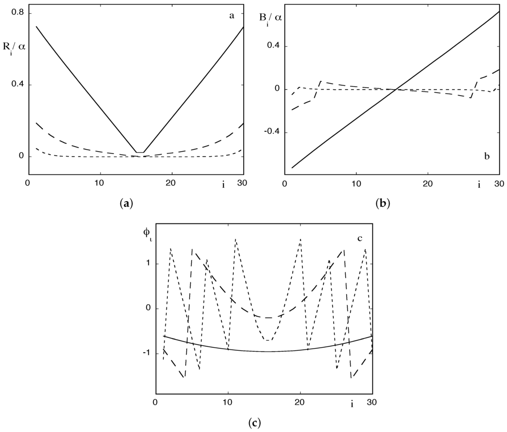
Figure 1. Amplitude scaled by $\alpha =2ϵ\mathrm{\Delta }x/q^2$: (a) of the response $R_i$ (Equation (11c)); (b) of the coefficient $B_i$ (Equation (12)); and (c) the behavior of the phase ${\varphi }_i$ (Equation (11d)) in the case of $n=30$ coexisting stable states for different values of the ratio $\omega /k_0$ = 0.01 (full lines), 0.1 (dashed lines) and 1 (dotted lines).

3. Multistability, Information Entropy, Information Production and Information Transfer

In this section, we introduce a set of quantities serving as measures of the choice and unexpectedness associated with self-organization and, in particular, with the multiplicity of available states of the system introduced in Section 2. We start with information (Shannon) entropy [1,2,3,4]:

$$\begin{array}{c}\hfill S_I=-\sum _{i=1}^n{p}_{i}ln{p}_i\end{array}$$

(14)

where the probabilities $p_i$ of the various states are defined by Equations (5), (9b) and (11). As a reference, we notice that in the absence of the nonequilibrium constraint provided by the external forcing, the probabilities are uniform, $p_i=1/n$, and $S_I$ in this state of full randomness attains its maximum value:

$$\begin{array}{c}\hfill S_{I,\max }=lnn\end{array}$$

(15)

The deviation from full randomness, and thus, the ability to reduce errors, is conveniently measured by the redundancy:

$$\begin{array}{c}\hfill R=1-\frac{S_I}{S_{I,\max }}=1-\frac{S_I}{lnn}\end{array}$$

(16)

We come next to the link with dynamics. Differentiating both sides of Equation (14) with respect to time and utilizing Equation (5), we obtain a balance equation for the rate of change of $S_I$.

$$\begin{array}{ccc}\hfill \frac{d{S}_I}{dt}& =& -\sum _i\frac{d{p}_i}{dt}ln{p}_i\hfill \\ & =& -\sum _{ij}{T}_{ij}{p}_{j}ln{p}_i\hfill \end{array}$$

Setting:

$$\begin{array}{ccc}\hfill T_{ij}& =& w_{ij}i\ne j\hfill \\ \mathrm{(17)}& \hfill T_{ii}& =& -\sum _{i\ne j}{T}_{ji}=w_{ii}\hfill \end{array}$$

we can rewrite this equation in the more suggestive form:

$$\begin{array}{ccc}\hfill \frac{d{S}_I}{dt}& =& -\sum _{ij}ln{p}_i(w_{ij}{p}_j-w_{ji}{p}_i)\hfill \\ & =& \frac{1}{2}\sum _{ij}ln\frac{p_j}{p_i}(w_{ij}{p}_j-w_{ji}{p}_i)\hfill \end{array}$$

Writing:

$$\begin{array}{c}\hfill ln\frac{p_j}{p_i}=ln\frac{w_{ij}{p}_j}{w_{ji}{p}_i}-ln\frac{w_{ij}}{w_{ji}}\end{array}$$

we finally obtain:

$$\begin{array}{c}\hfill \frac{d{S}_I}{dt}={\sigma }_I+J_I\end{array}$$

(18a)

where the information entropy production ${\sigma }_I$ and the associated flux $J_I$ are defined by [8,9]:

$$\begin{array}{c}\hfill {\sigma }_I=\frac{1}{2}\sum _{ij}(w_{ij}{p}_j-w_{ji}{p}_i)ln\frac{w_{ij}{p}_j}{w_{ji}{p}_i}\ge 0\end{array}$$

(18b)

$$\begin{array}{c}\hfill J_I=\frac{1}{2}\sum _{ij}(w_{ij}{p}_j-w_{ji}{p}_i)ln\frac{w_{ij}}{w_{ji}}\end{array}$$

(18c)

We notice the bilinear structure of ${\sigma }_I$ in which the factors within the sum can be viewed as generalized (probability) fluxes and their associated generalized forces. This is reminiscent of the expression of entropy production of classical irreversible thermodynamics [10]. As a reference, in the state of equipartition realized in the absence of the external forcing, one has $p_i=1/n$, $w_{ij}=k_0$, and ${\sigma }_I$ vanishes along with all individual generalized fluxes and forces. This property of detailed balance, characteristic of thermodynamic equilibrium, breaks down in the presence of the forcing, which introduces a differentiation in $p_i$ and an asymmetry in the $w_{ij}$. ${\sigma }_I$ measures, therefore the distance between equilibrium and nonequilibrium on the one side and between direct (i to j) and reverse (j to i) process on the other. In this latter context ${\sigma }_I$ is also closely related to the Kullback information.

Finally, in an information theory perspective, one is led to consider the information transfer between a part of the system playing the role of “transmitting set” X and a “receiver set” Y separated by a “noisy channel” [2,4]. In the dynamical perspective developed in this work, the analogs are two states, say i and j, and a conditional probability matrix, $W=\left\{W_{ji}\right\}$. The information transfer is then simply the sum of the Shannon entropy and the Kolmogorov–Sinai entropy [1,4]:

$$\begin{array}{c}\hfill h=-\sum _{ij}{p}_i{W}_{ji}ln{W}_{ji}\end{array}$$

(19)

To relate h with the quantities governing the evolution of our multistable system, we need to relate the transition probabilities $W_{ij}$ to the transition rates (probabilities per unit time) $w_{ij}$ featured in Equations (6) and (17). This requires in turn to map the continuous time process of the previous section to a discrete-time Markov chain. To this end, we introduce the discretized expression of the time derivative in Equation (5), utilize Equation (17) and choose the time step $\mathrm{\Delta }t$ as a fraction of the Kramers time associated with the passage over the potential barriers as discussed in Section 2:

$$\begin{array}{c}\hfill \mathrm{\Delta }t={(k_{i,i+1}+k_{i+1,i}+k_{i,i-1}+k_{i-1,i})}^{-1}={\kappa }^{-1}\end{array}$$

(20)

This leads to the discrete master-type equation:

$$\begin{array}{c}\hfill p_i(t+\mathrm{\Delta }t)=\sum _j{W}_{ij}{p}_j\left(t\right)\end{array}$$

(21)

where the stochastic matrix W is defined by:

$$\begin{array}{ccc}\hfill W_{i\pm 1,i}& =& \frac{k_{i,i\pm 1}}{\kappa }\hfill \\ \mathrm{(22a)}& \hfill W_{ii}& =& \frac{k_{i+1,i}+k_{i-1,i}}{\kappa }2\le i\le n-1\hfill \end{array}$$

$$\begin{array}{c}\hfill W_{21}=\frac{k_{12}}{\kappa },W_{11}=1-\frac{k_{12}}{\kappa }\end{array}$$

(22b)

$$\begin{array}{c}\hfill W_{n-1,n}=\frac{k_{n,n-1}}{\kappa },W_{nn}=1-\frac{k_{n,n-1}}{\kappa }\end{array}$$

(22c)

Introducing again as a reference the state in the absence of the forcing, one sees straightforwardly that $k_{ij}=k_0$, $p_i=1/n$ and $W_{ij}=1/4$ for $i\ne j$, $W_{ii}=1/2$ for $2\le i\le n-1$ and $W_{11}=W_{nn}=3/4$. Expression (19) reduces then to:

$$\begin{array}{c}\hfill h^{\left(0\right)}=\frac{n-2}{2}·\frac{3}{2}ln2+\frac{1}{n}(-\frac{3}{2}ln3+4ln2)\end{array}$$

(23)

where the two terms on the right-hand side account, respectively, for the contributions of the intermediate states and of the boundary states one and n.

It is worth noting that for n, even the Markov chain associated with the forcing-free system is lumpable [11], in the sense that upon grouping the original states, one can reduce Equation (21) into a system of just two states a and b, with $W_{aa}=W_{bb}=3/4$ and $W_{ab}=W_{ba}=1/4$. In other words, in the absence of the nonequilibrium constraint, the intermediate states play no role. The presence of the forcing will change this situation radically by inducing non-trivial correlations and information exchanges within the system.

4. Nonequilibrium Dynamics of Information and Stochastic Resonance

Our next step is to evaluate the quantities introduced in the preceding section in the presence of the nonequilibrium constraint provided by the external forcing with emphasis on the roles of key parameters, such as forcing amplitude and frequency, noise strength and number of states.

4.1. Information Entropy and Redundancy

Substituting expression Equation (9b) into Equation (14) and using the property ${\sum }_i\delta p_i=0$, one sees straightforwardly that the $O\left(ϵ\right)$ contributions to $S_I$ cancel identically. Keeping the first non-trivial (i.e., $O\left({ϵ}^2\right)$) parts, one obtains:

$$\begin{array}{c}\hfill S_I=S_I^{\left(0\right)}+\mathrm{\Delta }{S}_I\end{array}$$

(24a)

where:

$$\begin{array}{c}\hfill S_I^{\left(0\right)}=S_{I,\max }=lnn\end{array}$$

(24b)

and:

$$\begin{array}{c}\hfill \mathrm{\Delta }{S}_I=-\frac{n}{2}\sum _i\delta p_i^2\end{array}$$

(24c)

Using expression Equation (11b) for $\delta p_i$, we may further decompose $\mathrm{\Delta }{S}_I$ into its time average part $\overline{\mathrm{\Delta }{S}_I}$ and a periodic modulation $\delta S_I$ around the average:

$$\begin{array}{c}\hfill \overline{\mathrm{\Delta }{S}_I}=-\frac{{ϵ}^{2}n}{4}\sum _i{R}_i^2\end{array}$$

(25a)

$$\begin{array}{ccc}\hfill \delta S_I& =& \frac{{ϵ}^{2}n}{4}\sum _i{R}_i^{2}cos\left(2(\omega t+{\varphi }_i)\right)\hfill \\ \mathrm{(25b)}& & =& R_{\mathrm{eff}}^{2}cos(2\omega t+{\psi }_{\mathrm{eff}})\hfill \end{array}$$

where the effective amplitude $R_{\mathrm{eff}}$ and phase ${\psi }_{\mathrm{eff}}$ of the modulation are expressed in terms of $R_i$ and ${\varphi }_i$.

The evaluation of the redundancy, Equation (16), follows straightforwardly from that of $S_I$, leading to:

$$\begin{array}{c}\hfill R=-\frac{\mathrm{\Delta }{S}_I}{lnn}\end{array}$$

(26)

where $\mathrm{\Delta }{S}_I$ is given by Equations (24c) and (25).

In Figure 2a,b, the time averaged excess entropy $\overline{\mathrm{\Delta }{S}_I}$ and redundancy $\overline{R}$ are plotted as a function of the number n of states using expressions Equations (11)–(13). In all cases, $\overline{\mathrm{\Delta }{S}_I}$ is negative and $\overline{R}$ positive, reflecting the enhancement of predictability induced by the nonequilibrium constraint. Furthermore, and similarly to Figure 1a, for given noise strength $q^2$, the enhancement is more pronounced in the range of low frequencies ω and is further amplified when the conditions of stochastic resonance are met. Interestingly, for given $q^2$ and ω, the enhancement exhibits a clear-cut extremum for a particular value of the number of states. This unexpected result suggests that to optimize its function our multistable system, viewed as an information processor, should preferably be endowed with a number of states (essentially a “variety”) that is neither very small nor too large. Finally in Figure 3, the time evolution of the full $\mathrm{\Delta }{S}_I$ in the low frequency range is plotted using expression Equations (11)–(13) and (25).

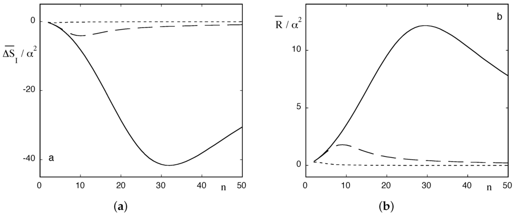
Figure 2. Time average excess entropy $\overline{\mathrm{\Delta }{S}_I}$ (Equation (25a)) (a) and redundancy $\overline{R}$ (Equation (26)); (b) as a function of the number n of states present for different values of the ratio $\omega /k_0$= 0.01 (full lines), 0.1 (dashed lines) and 1 (dotted lines). Normalization parameter α as in Figure 1.

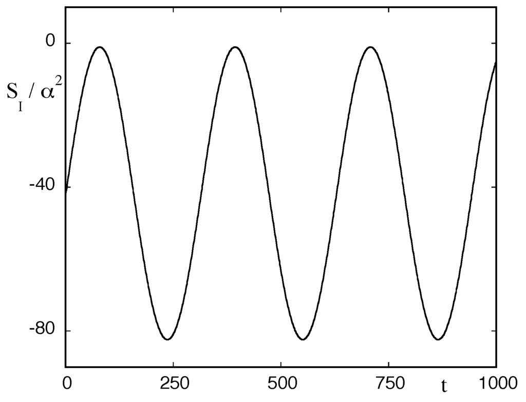
Figure 3. Time evolution of the full excess entropy $\mathrm{\Delta }{S}_I$ (Equation (24c)) in the case of $n=32$ coexisting states with $\omega /k_0$ = 0.01, corresponding to the minimum of the full line of Figure 2a.

4.2. Information Entropy Production

Our starting point is Equation (18b). We have shown in the preceding section that the zeroth order part of ${\sigma }_I$ vanishes, since it corresponds to a state where detailed balance holds. To obtain the first non-trivial contribution, we need therefore to expand both $p_i$ and $w_{ij}$ in the forcing amplitude ϵ. Actually, since each of the two factors in the expression of ${\sigma }_I$ vanishes for $ϵ=0$, it suffices to take each of them to $O\left(ϵ\right)$ in order to obtain the dominant, $O\left({ϵ}^2\right)$ contribution. Substituting Equation (9b) along with the analogous expressions for $w_{ij}$:

$$\begin{array}{c}\hfill w_{ij}=w_{ij}^{\left(0\right)}+\delta w_{ij}(j=i\pm 1)\end{array}$$

(27)

where $w_{ij}^{\left(0\right)}=k_0$ and $p_0=1/n$, we obtain:

$$\begin{array}{ccc}\hfill \mathrm{\Delta }{\sigma }_I& =& \frac{n}{2k_0}\{\sum _i{[k_0(\delta p_{i+1}-\delta p_i)+\frac{1}{n}(\delta w_{i,i+1}-\delta w_{i+1,i})]}^2\hfill \\ \mathrm{(28)}& & +& \sum _i{[k_0(\delta p_{i-1}-\delta p_i)+\frac{1}{n}(\delta w_{i,i-1}-\delta w_{i-1,i})]}^2\}\hfill \end{array}$$

where $\delta p_i$ is given by Equations (11)–(13) and (see Equations (6), (7) and (17)):

$$\begin{array}{c}\hfill \delta w_{i,i\pm 1}=\pm ϵ\frac{2}{q^2}{k}_0\pi sin\omega t\end{array}$$

(29)

Taking the time average $\overline{\mathrm{\Delta }{\sigma }_I}$ over a period of the forcing and denoting for compactness sign $B_i=s_i$, one finally obtains:

$$\begin{array}{ccc}\frac{\overline{\mathrm{\Delta }{\sigma }_I}}{{ϵ}^2/\left(2k_0\right)}\hfill & =\hfill & \frac{16k_0^2{\pi }^2(n-1)}{n{q}^4}\hfill \\ & +\hfill & k_0^{2}n(\frac{1}{2}(R_1^2+R_2^2)-s_1{s}_2{R}_1{R}_{2}cos({\varphi }_2-{\varphi }_1))\hfill \\ & +\hfill & \frac{4k_0^2\pi }{q^2}(s_2{R}_{2}cos{\varphi }_2-s_1{R}_{1}cos{\varphi }_1)\hfill \\ & +\hfill & k_0^{2}n(\frac{1}{2}(R_{n-1}^2+R_n^2)-s_{n-1}{s}_n{R}_{n-1}{R}_{n}cos({\varphi }_{n-1}-{\varphi }_n))\hfill \\ & +\hfill & \frac{4k_0^2\pi }{q^2}(s_{n-1}{R}_{n-1}cos{\varphi }_{n-1}-s_n{R}_{n}cos{\varphi }_n)\hfill \\ & +\hfill & {\sum }_{i=2}^{n-1}\{k_0^{2}n[\frac{1}{2}(R_{i+1}^2+R_{i-1}^2+2R_i^2)-s_i{R}_i(s_{i+1}{R}_{i+1}cos({\varphi }_{i+1}-{\varphi }_i)\hfill \\ & +\hfill & s_{i-1}{R}_{i-1}cos({\varphi }_{i-1}-{\varphi }_i)\left)\right]\hfill \\ & +\hfill & \frac{4k_0^2\pi }{q^2}(s_i{R}_{i+1}cos{\varphi }_{i+1}-s_{i-1}{R}_{i-1}cos{\varphi }_{i-1})\}\hfill \end{array}$$

(30)

Figure 4 depicts the dependence of $\overline{\mathrm{\Delta }{\sigma }_I}$, scaled by the factor $2k_0{(ϵ\pi /q^2)}^2$, as a function of a number of states n for different values of the forcing frequency. We observe a trend similar to that of Figure 2a,b: an enhancement under nonequilibrium conditions near stochastic resonance for an optimal number of intermediate states and practically no effect of the nonequilibrium constraint for higher frequencies. Since the time average of $d{S}_I/dt$ in Equation (18a) is necessarily zero, it follows that the information flux $J_I$ (Equation(18c)) will display a similar behavior albeit with an opposite sign, i.e., a pronounced dip for low frequencies and for an optimal number of states. In a sense, the excess information produced remains confined within the system at the expense of a negative excess information flux, in much the same way as in the entropy balance of classical irreversible thermodynamics [10].

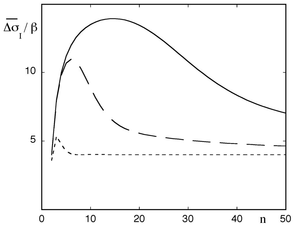
Figure 4. Information entropy production averaged over the period of the forcing (Equation (30)), scaled by $\beta =2k_0(ϵ\pi /q^2{)}^2$ as a function of the number of states n present and for different values of the ratio $\omega /k_0$ = 0.01 (full line), 0.1 (dashed line) and 1 (dotted line).

4.3. Information Transfer and Kolmogorov–Sinai Entropy

We begin by decomposing $p_i$ and $W_{ij}$ in Equation (19) into a reference part and a deviation arising from the presence of the nonequilibrium constraint:

$$\begin{array}{c}\hfill p_i=p_i^{\left(0\right)}+\delta p_i{W}_{ij}=W_{ij}^{\left(0\right)}+\delta W_{ij}\end{array}$$

(31)

where $p_i^{\left(0\right)}=1/n$ and the $W_{ij}^{\left(0\right)}$’s have been evaluated in Section 3. Using Equations (7), (8) and (22), one can establish the following properties:

• $\delta W_{ii}$ vanish for the intermediate states $2\le i\le n-1$.
• The contributions of $k_{i,i+1}$ coming from second order terms in the expansion of Equation ((7a) in powers of ϵ do not contribute up to order ${ϵ}^3$ to $\delta W_{i,i\pm 1}$, which can therefore be limited for our purposes to its first order in ϵ part $\delta W_{i,i\pm 1}^{\left(1\right)}$.
• $\delta W_{i,i\pm 1}^{\left(1\right)}$, $\delta W_{11}$ and $\delta W_{nn}$ satisfy the symmetry relations:

  $$\begin{array}{ccc}\delta W_{i,i+1}^{\left(1\right)}\hfill & =\hfill & -\delta W_{i,i-1}^{\left(1\right)}=\delta W\hfill \\ \delta W_{11}\hfill & =\hfill & -\delta W_{nn}=-\delta W\hfill \end{array}$$

  (32)

Substituting into Equation (19) and using the symmetry property $\delta p_n=-\delta p_1$ along with the normalization condition ${\sum }_{i=1}^n\delta p_i=0$, one obtains after some straightforward manipulations:

$$\begin{array}{c}\hfill h=h^{\left(0\right)}+[2ln3\delta W\delta p_1-\frac{4}{n}(n-\frac{2}{3})\delta W^2]\end{array}$$

(33)

with:

$$\begin{array}{c}\delta p_1=ϵ\left(\mathrm{sign}{B}_1\right)R_{1}sin\left(\omega t+{\varphi }_1\right)\\ \delta W=\frac{\delta k_{i,i+1}}{4k_0}=ϵ\frac{1}{4}\frac{2\pi }{q^2}sin\omega t\end{array}$$

(34)

Taking the average of Equation (33) over a period of the forcing leads to the following expression for the mean excess Kolmogorov–Sinai entropy:

$$\begin{array}{c}\hfill \overline{\mathrm{\Delta }h}=\overline{h}-h^{\left(0\right)}={ϵ}^2\{ln3\frac{\pi }{2q^2}\mathrm{sign}{B}_1{R}_{1}cos{\varphi }_1-\frac{2}{n}(n-\frac{2}{3})\frac{{\pi }^2}{4q^4}\}\end{array}$$

(35)

In Figure 5, the dependence of $\overline{\mathrm{\Delta }h}$, scaled by a factor ${\alpha }^2={ϵ}^{2}4{\pi }^2/q^4$, on the number of states is plotted for various values of the forcing frequency. We find a trend similar to the one in Figure 2, Figure 3 and Figure 4, namely an optimal response for frequency values close to conditions of stochastic resonance and for a particular number of intermediate states. The negative values of $\overline{\mathrm{\Delta }h}$ reflect the reduction of randomness (of which h is a characteristic measure) induced by the nonequilibrium constraint.

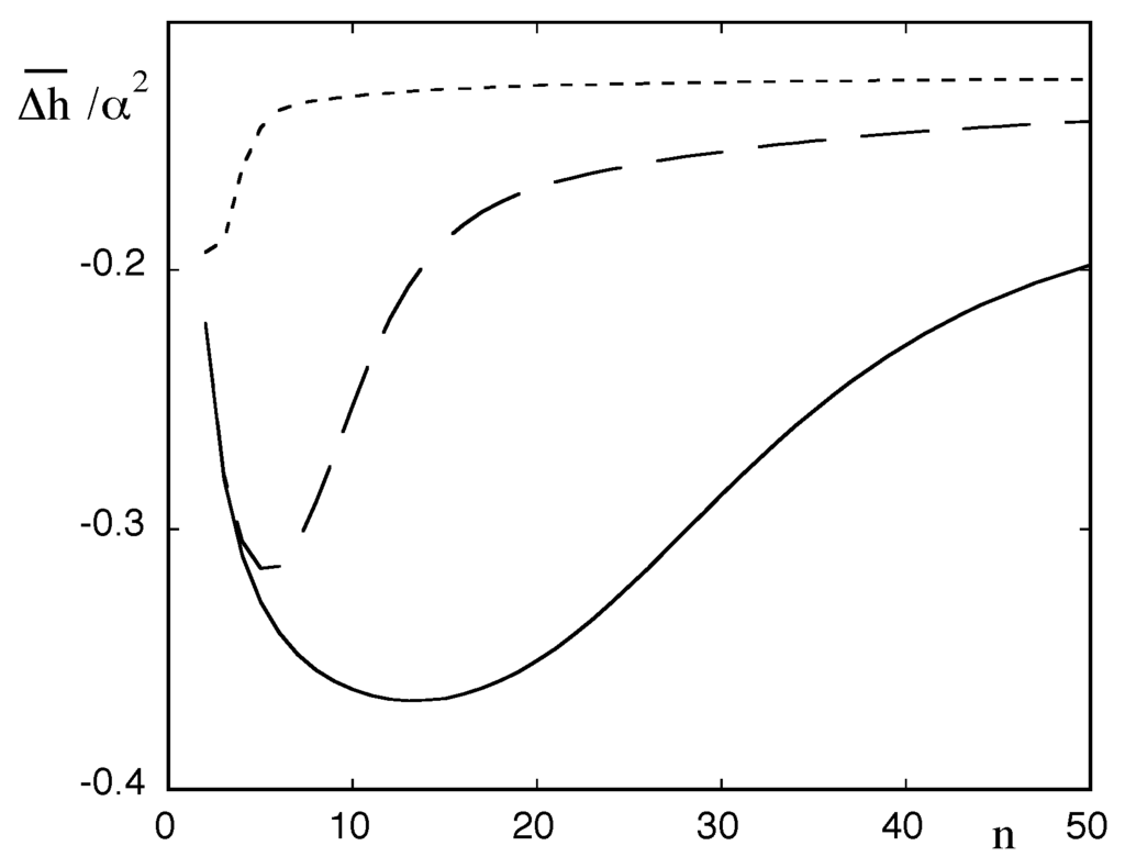
Figure 5. Kolmogorov–Sinai entropy averaged over the period of the forcing (Equation (35)) as a function of the number of states n present and for different values of the ratio $\omega /k_0$ = 0.01 (full line), 0.1 (dashed line) and 1 (dotted line). Normalization parameter α as in Figure 1.

5. Conclusions

In this work, a nonlinear system subjected to a nonequilibrium constraint in the form of a periodic forcing, giving rise to complex behavior in the form of fluctuation-induced transitions between multiple steady states and of stochastic resonance, was considered. Mapping the dynamics into a discrete-state Markov process allowed us to view the system as an information processor. Subsequently, the link between the dynamics and, in particular, the self-organization induced by the nonequilibrium constraint, on the one side, and quantities of interest in information theory, on the other side, was addressed. It was shown that the nonequilibrium constraint leaves a clear-cut signature on these quantities by reducing randomness and by enhancing predictability, which is maximized under conditions of stochastic resonance. Of special interest is the a priori unexpected existence of an optimum for a particular number of simultaneously stable states suggesting the existence of optimal alphabets on which information is to be generated and transmitted.

In summary, it appears that when viewed in a dynamical perspective, generalized entropy-like quantities as used in information theory can provide useful characterizations of self-organizing systems led to choose among a multiplicity of possible outcomes. Conversely and in line with the pioneering work in [3,4], information constitutes in turn one of the basic attributes emerging out of the dynamics of wide classes of self-organizing systems and conveying to them their specificity.

References

- Nicolis, G.; Nicolis, C. Foundations of Complex Systems, 2nd ed.; World Scientific: Singapore, Singapore, 2012. [Google Scholar]
- Ash, R.B. Information Theory; Dover: New York, NY, USA, 1990. [Google Scholar]
- Haken, H. Information and Self-Organization; Springer: Berlin, Germany, 1988. [Google Scholar]
- Nicolis, J.S. Chaos and Information Processing; World Scientific: Singapore, Singapore, 1999. [Google Scholar]
- Gardiner, C. Handbook of Stochastic Methods; Springer: Berlin, Germany, 1983. [Google Scholar]
- Gammaitoni, L.; Hänggi, P.; Jung, P.; Marchesoni, F. Stochastic resonance. Rev. Mod. Phys. 1998, 70, 223–287. [Google Scholar] [CrossRef]
- Nicolis, C. Stochastic resonance in multistable systems: The role of intermediate states. Phy. Rev. E 2010, 82, 011139. [Google Scholar] [CrossRef] [PubMed]
- Luo, J.L.; van den Broeck, C.; Nicolis, G. Stability criteria and fluctuations around nonequilibrium states. Z. Phys. B 1984, 56, 165–170. [Google Scholar]
- Gaspard, P. Time-reversed dynamical entropy and irreversibility in Markovian random processes. J. Stat. Phys. 2004, 117, 599–615. [Google Scholar] [CrossRef]
- De Groot, S.; Mazur, P. Nonequilibrium Thermodynamics; North Holland: Amsterdam, The Netherlands, 1962. [Google Scholar]
- Kemeny, J.; Snell, J. Finite Markov Chains; Springer: Berlin, Germany, 1976. [Google Scholar]
© 2016 by the authors; licensee MDPI, Basel, Switzerland. This article is an open access article distributed under the terms and conditions of the Creative Commons Attribution (CC-BY) license (http://creativecommons.org/licenses/by/4.0/).