Abstract
Theories and numerical models of atmospheres and oceans are based on classical mechanics with added parameterizations to represent subgrid variability. Reformulated in terms of derivatives of information entropy with respect to large scale configurations, we find systematic forces very different from those usually assumed. Two examples are given. We see that entropic forcing by ocean eddies systematically drives, rather than retards, large scale circulation. Additionally we find that small scale turbulence systematically drives up gradient (“un-mixing”) fluxes. Such results confront usual understanding and modeling practice.
1. Geophysical Fluid Dynamics (GFD), Based on Classical Mechanics
Seeking to characterize the large scale evolution of atmospheres or oceans, GFD is based on classical fluid mechanics under influences of gravity and rotation. As an exercise of classical mechanics, GFD is deterministic. Equations are written as though all macroscopic degrees of freedom are explicitly represented. The only uncertainty is that scales of molecular motion are subsumed under the continuum hypothesis with well-tested representations in terms of thermal conductivity or viscosity, for examples.
In practice, GFD is almost never exercised on scales for which complete representation of all macroscopic motion is possible. The only exceptions occur when GFD is applied in numerical models of laminar flows in rotating tank experiments on scales for which “molecular” coefficients for viscosity or haline conduction can be applied. In “real world” applications, the scales of motion that can be resolved on even the most powerful computers are only the tiniest fraction of the macroscopic variability actually present. Atmosphere, oceans and even most duck ponds are simply way too large for the theories and numerical methods that are applied. As example, Earth’s oceans exhibit something like 1025 to 1030 degrees of freedom (taking into account only the fields of velocity, temperature and salinity). The largest ocean models to date consider 109 to 1010 variables to define the ocean state. Thus, for any one variable retained explicitly, there are at least 1015 variables unknown (not counting very many more molecular degrees of freedom). What to do?
This circumstance has a long history, often called subgridscale (SGS) parameterization. The simplest, and still among the most common, “fix” for SGS is to write the GFD equations as though everything was resolved down to the scale of continuum hypothesis (averaging over molecular motions), but then to replace coefficients of viscosity or of thermal conductivity with adjustable coefficients several orders of magnitude larger, effectively treating macroscopic variability on SGS as a sort of super molecular variability. Because SGS issues arise throughout fields of fluids engineering, there have been vastly many studies seeking to refine parameterizations, usually be seeking a dependence of the parameters upon the larger scale, resolved environment. In engineering applications, SGS can be quite sophisticated with extensive empirical adjustment.
In atmospheric application, there has been opportunity for empirical adjustment to SGS schemes on account on numerical weather forecasting with daily validation. However, for longer term projections of climate change and in ocean modeling, an empirical basis for refining SGS schemes is difficult.
It is hoped that this article may be of interest to readers of Entropy for two reasons. First, we’ll see some attempts to improve upon SGS by taking explicit account of entropy calculus. The limited extent of these efforts to date may encourage some readers to join in a stronger overall effort. Second, it may be startling when phenomena such as organizing roles of entropy, as known e.g. at nanoscales, are seen again on planetary scales, such as when entropy organizes ocean circulation.
2. Early Indications, Extremal Principles
There have been indications that entropy can guide understanding of GFD, with entropy:
where dP integrates over probabilities of all possible configurations. Two quite different approaches have been taken.
H = −∫dPlogP
Considering uncertainty only on molecular scales, (1) provides a basis for traditional thermo-dynamic entropy. Pioneering papers [1,2] have argued that the mean state of the atmosphere is close to that which maximizes production of thermodynamic entropy. Further researches along these lines are reviewed, e.g., [3], while the logical basis for maximizing entropy production (MEP) has been strengthened [4,5,6,7].
Alternatively and omitting thermodynamic entropy altogether, [8] considered (1) based on uncertainty of fluctuations on macroscales for an idealized (quasigeostrophic) ocean. This and other early works, reviewed at [9], considered the maximum of entropy (ME) rather than MEP. ME solutions in GFD continue to hold interest [10,11].
We see nearly antipodal approaches: on one hand taking no account of entropy associated with macroscale fluctuations while maximizing production of thermodynamic entropy; on the other hand discarding thermodynamic entropy while maximizing entropy (not entropy production) due to macroscale fluctuations. Each approach claims successes characterizing the climate system. Can both be correct, as far as they go? Can we go further?
Among difficulties with extremal principles is that answers have a “take it or leave it” air. If one contemplates Earth’s atmosphere and ocean, so well as these can be observed, and asks “what next?”, we turn to general circulation models (GCMs) which seek to solve equations of motion under explicit forcing. Results may resemble somewhat certain ME and MEP states, and this may be encouraging in terms of interpretive guidance. We wish to go further.
3. Turbulence Closure Theory
This is a subject recently reviewed [12] in Entropy. Present comments will be brief. Since pioneering work [13,14], a wealth of studies have been performed for statistically homogenous turbulence in 3D and in 2D, the latter suggestive of large scale eddies in atmospheres and oceans. Closure theory for 2D turbulence has been extended to include many geophysical effects including differential rotation (on beta-plane or on sphere), baroclinicity and bottom topography.
While turbulence closure theory developed largely independently of entropy considerations, an important connection was established [15] showing that a broad class of closure theories strictly implied a Boltzmann H theorem, i.e., entropy (1) is non-decreasing:
on account of interactions among turbulent fluctuations. In isolation from forcing and dissipation, (2) implies evolution toward ME solutions cited previously. However closure theory allows external (stochastic) forcing as well as explicit representation of dissipation, losing energy from macroscale fluctuations to the field of (implied) molecular agitation. Then the part of H due to macroscale fluctuations satisfies a budget with a source term given by external (stochastic) forcing, an internal production term due to turbulent interactions, and a loss term by dissipation.
dH/dt ≥ 0
For such theories the connection with entropy is explicit and can be further explored. At the very least a 2nd Law statement (2) can be proven. This is important because, for the vastly many SGS schemes used in GCMs, no 2nd Law consistency is considered and indeed is demonstrably violated in some cases.
The huge challenge for closures that have followed since [13,14] is their technical difficulty. Only special circumstances such as statistically homogenous and nearly isotropic turbulence have been amenable to careful investigation. Attempts are made to overcome these limitations, as perhaps seen in a series of papers [16,17,18,19]. This approach has allowed investigators (see [19] and references therein) to include mean zonal flow, sphericity (or beta effect) and bottom topography.
To make calculations more amenable, [16] introduced a quasi-diagonal approximation, “QDIA”, assuming that second order correlations between coefficients at different wavevectors can be represented by correlations only at the same wavevector. This was used in later studies summarized in [19]. However, even with simplifying assumptions such as QDIA, the technical difficulty in closures has so far prevented practical application in GCMs.
4. Entropy Gradients and Generalized Forces
Three challenges are:
- 1)
- to utilize full information theoretic entropy (1), including both thermodynamics and macroscale variability,
- 2)
- to address the non-equilibrium, open nature of the Sun - Earth - atmosphere - ocean - space system, and
- 3)
- to deliver practical results, for example to measurably improve the fidelity of GCMs.
Usually we write, then hope to solve, equations of motion for how things change, where “things” might be flow fields, temperature fields, etc. We might write:
where Y is the collection of fields of interest, perhaps momentum, temperature, etc. F(Y) expresses the linear and nonlinear dependence of ∂Y/∂t upon Y, and G expresses external forces that may be independent of Y. Especially the science of GFD provides the dynamic core for GCMs by writing (3) for the coupled fields of momentum and density under the influences of gravity and planetary rotation. viz.:
 where ∂t denotes partial derivative with respect to time, u is velocity, ∇ is spatial gradient, Ω is coordinate rotation rate, p is pressure, ρ is density, Φ is generalized gravitational potential (includes coordinate rotation and tidal forcing), υ is coefficient of viscosity (kinematic units), ∇2≡∇·∇, T is potential temperature (after adiabatic adjustment to a reference pressure), κ is coefficient of thermal conduction (kinematic units), Q represents internal source of heat, and an equation of state, ρ = ρ (T,p), couples (4a) and (4b). Depending upon applications, there may be more coupled equations such as for moisture in the atmosphere, salinity in the oceans, etc.
∂Y/∂t = F(Y) + G
(∂t + u·∇)T = κ∇2T + Q
Based in classical mechanics, there is well-established confidence in the derivation of (4). We should be cautious though. Eqn. (4) is a partial differential equation, yet the basis for (4) does not allow true differentials (infinitesimal differences across infinitesimal displacements). Rather (4) already requires that the least allowed displacement be very much larger than distances among molecules in the fluid, i.e., we take a continuum assumption. In many cases this assumption is quite secure and coefficients such as υ or κ in (4) have values well observed (not derived!) from laboratory studies.
Here we do not question this continuum assumption. Instead we recognize that there is no feasible way, theoretically or numerically, to solve (4) in a domain such as an atmosphere or an ocean or a lake or even a modest duck pond at the length scales for which (4) would be valid. That is, one would solve down to length scales at which u and θ should vary so smoothly that differences over finite displacements would approximate derivatives. Historically we’ve done something else, replacing measurable coefficients υ or κ with artificial coefficients typically several orders of magnitude larger than the measured coefficients, rewriting (4) as:
 where Am and Ah are second order tensors which are usually assumed to be anisotropic, possibly with symmetric and anti-symmetric parts, with coefficients that may vary in space and time, perhaps depending upon properties of large scale u and T. Two arguments are often given for rewriting (4) to (5). First, one must do something like this to make models (e.g., GCMs) work. Second, coefficients in Am or Ah are supposed to represent effects of subgridscale fluctuations in u and T which are believed to generally “mix away” large scale property gradients. Efforts to find suitable expressions for coefficients in Am or Ah have been the subject of the huge SGS research mentioned in Sect. 1. A great deal of plausible thinking and post hoc corrections have gone into the many schemes for Am or Ah. Yet what is striking is the absence of consideration for entropic calculus or even for consistency with Second Law (2). We can and should do better.
(∂t + u·∇)T = ∇·(Ah∇T) + Q
A very first step is to recognize more clearly what are the dependent variables for which we would solve. Regarding output from a GCM, we might view maps of u or T. Are fields of u and T the dependent variables? That is, is T(x,t) a prediction for the precise temperature at a precise point at a precise time? No. Modellers sometimes retreat to a modelling answer, possibly viewing T as the ratio of heat content to thermal mass in a model’s cell that might be some 10 s of km in horizontal extent and 10 s to 100 s of m in vertical. Unhappily, an integral operator which could extract cell heat content (say) cannot be passed over (4) in a way that obtains complete (closed) expressions. One is left to guessing, much as we were guessing at (5).
Alternatively we recognize from the outset that we make calculations in the absence of full information. All of the degrees of freedom, both in the molecular field and in the macroscale variability on length scales too small to be explicitly represented, are known only in probability. Fields such as u or T are moments over the probabilities of all possible realizations of subgrid fluctuations. Rather than speaking of a “temperature equation”, if we were obliged to speak of “the equation for the temperature moment over the probabilities of ...”, we might sooner have been skeptical about equations such as (5). Of course it is much easier to say “temperature equation”. Yet, when we realize that we seek equations of the evolution of moments of probabilities, we are more ready to consider entropic effects absent from classical mechanics.
Taking u and T, understood as moments over probabilities, for Y, many of the terms seen in (4) or (5) are part of ∂Y/∂t, cf. (3). Linear terms appear just as in (4) or (5), and nonlinearities whereby large scale moment fields interact with large scale moment fields also appear as in (4) or (5). But there is more. The aggregate effect of the myriad subgrid fluctuations also affect ∂Y/∂t. How? The suggestion here is that the gradient of entropy with respect to the moment fields act as a forcing upon the moment fields. That is, insofar as total entropy depends upon configurations of moment fields, if a hypothetical small change δY to Y yields a change δH in entropy, then an entropic force δH/δY acts to drive ∂Y/∂t. Symbolically:
where ∂YH is the gradient of H with respect to the fields that form Y. C is an operator projecting ∂YH onto ∂Y/∂t .
∂Y/∂t = F(Y) + G + C·∂YH
The great challenge is to move from (6), which is only symbolic, to actual calculation. Two approaches are feasible. Observing that C·∂YH acts to drive Y toward higher entropy, we can try to replace C·∂YH with a MEP term. Difficulties in GFD context are to obtain a valid expression for entropy production and to maximize that subject to suitable constraints. Partial progress has been made in this way, e.g., [20,21,22]. For the present, we will attempt to address the entropy gradient terms in (6) directly. It will be seen in Section 5.1 that the present method and MEP yield very similar results.
The first step is to recognize that C·∂YH has two parts, C and ∂YH. While some components of ∂YH may be very large, if the elements in C which project ∂YH onto ∂Y/∂t are extremely small, then these large ∂YH are not very effective. In the case of oceans, a huge increase in entropy could be realized if the oceans (in “thought experiment”) could come to absolute thermodynamic equilibrium (isothermal, in solid body rotation with Earth). However, the timescale to accomplish such adjustment, even assuming turbulent enhancement of macroscale dissipation via υ and κ, is enormous compared with vastly more rapid oceanic adjustments. Hence, as a practical step, we here omit thermodynamic contribution to H, retaining only the part due to macroscale variability.
Notably, the choice here to omit thermodynamic H is exactly opposite from choices [1,2] and others who treat H as entirely thermodynamic without contribution from macroscale variability. These authors have constructed plausible distributions for Earth’s and other planetary atmospheres, as reviewed at [3], as well as idealized oceans [23] by maximizing production of thermodynamic H. Clearly the present paper, as well as those reviewed at [3], are incomplete and a more comprehensive account, retaining both thermodynamics and macroscale variability in H, remains a challenge to future researchers. For the present paper we will proceed from only the partial perspective arising from macroscale variability.
The rapid mechanism by which oceans can generate H is macroscale advection. On timescales from minutes (viz., internal gravity wave interactions) to weeks (viz., mesoscale eddy interactions), we may rearrange large volumes of seawater with very little thermodynamic modification. At first let us treat advection as ideal (adiabatic).
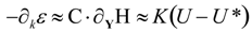
Seeking ways to render C·∂YH calculable, consider:

That is, we identify a locus, Y*, where ∂YH is small in the sense that ∂YH at Y* is very much weaker than ∂YH at Y. Identification of Y* depends upon rapid dynamical adjustments, influenced by gravity and planetary rotation, for example. We then estimate ∂YH at Y as proportional to the displacement Y*-Y. Having not yet obtained an expression for C or for ∂Y∂YH, we collapse these two into unknown operator K for which we will seek plausible “eddy scaling” representation.
Cautions are obvious. “≈” in (7) is an assumption more than an approximation, given that we make no assertion about how small is Y*-Y. Representations for Y* and K are developed in examples in the next section. As will be seen, such representations to date are crude (at best). Nonetheless improvements to GFD and to skill realized in practical models are seen. A hope is that such tangible progress will invite more critical attention to the sorts of developments which here must be described as rudimentary.
5. Two Examples
5.1. Neptune Effect: Entropic Forcing of Mean Ocean Circulation
This and the following section are drawn from oceans applications based upon this author’s familiarity. Implications for Earth’s atmosphere, other planetary flows and GFD generally will be apparent. First we consider “neptune effect”, so-called after a cartoon [24]. We will see the strong and largely unsuspected role of entropy organizing Earth’s mean ocean circulation along with a simple opportunity to correct, in part, ocean and climate models.
The theoretical basis for neptune follows from the quasigeostrophic barotropic vorticity equation, one of the fundamentals of GFD, recently discussed [12] in Entropy. Further simplifying from [12], we consider only:
 in Cartesian x,y coordinates where
  is the vertical component of relativity vorticity and ψ is the corresponding streamfunction for horizontal, nondivergent (in quasigeostrophic approximation) velocity, u. ∂(,)/∂(,) denotes the Jacobian determinant. The fluid, bounded above and below by rigid level planes is subject to uniform background rotation about vertical axis
  . h(x,y) appears in (8) when we allow one of the bounding planes to include small (with respect to separation between planes) deformations. Thus h(x,y) may represent bottom topography underlying an atmosphere or ocean in this approximation. At this point we put the right side of (8) to zero, i.e., considering only unforced, non-dissipative advection of potential vorticity, q = ζ + h.
is the vertical component of relativity vorticity and ψ is the corresponding streamfunction for horizontal, nondivergent (in quasigeostrophic approximation) velocity, u. ∂(,)/∂(,) denotes the Jacobian determinant. The fluid, bounded above and below by rigid level planes is subject to uniform background rotation about vertical axis . h(x,y) appears in (8) when we allow one of the bounding planes to include small (with respect to separation between planes) deformations. Thus h(x,y) may represent bottom topography underlying an atmosphere or ocean in this approximation. At this point we put the right side of (8) to zero, i.e., considering only unforced, non-dissipative advection of potential vorticity, q = ζ + h.There are two reasons to begin so simply as (8). First, we are isolating only mechanisms that allow rapid adjustments by advecting q.
Second, and possibly of special interest to readers of Entropy, we connect with two of the seminal papers of Onsager [25,26]. [25] considered (8) without h, i.e. supposing h=0, while treating the vorticity field as a collection of pointwise vortices each carrying integrated vorticity, termed circulation, Гi ≡ ∫dAζi where Гi is the circulation due to vorticity, ζi, of the ith point vortex and dA is an elemental area. (The problem is posed in two dimensions.) The collection of point vortices conserves interaction energy:
 where rij is the separation between ith and jth vortex. Depending on configurations of the vortices, E can take any value from - ∞ to ∞. But then the available phase space (here configuration space) is a function of E, taking a maximum at some E*. For E > E*, greater E would decrease available phases space, a circumstance of “negative temperature”. The result is that vortices of like sign tend to cluster, creating larger compound vortices (today we say “coherent structures”) while weaker vortices are more free to roam nearly randomly. In this way Onsager foresaw much of the literature of “two-dimensional turbulence” that would unfold over the subsequent half century.
[26] considered a different question: the orientation of rod-like particles in colloidal suspension. Entropy in this case depends upon the freedom of each rod to be nearly randomly located and nearly randomly oriented. If the density of rods is increased, there comes a point where restricting the freedom of orientation by forming patches of like-oriented rods (“nematic ordering”) makes available greater volume for more nearly random location. In this way Onsager foresaw much of the literature of “excluded volume effects” that play a role today understanding entropic forces in colloidal chemistry, microbiology and nanomechanics.
Onsager did not happen to include the role of bottom topography, h in (8), when he considered vortices. But we can imagine only a footnote in [25] if Onsager appended a collection of bound vortices (assigned to fixed locations) with circulations Ωk. Then there is interaction energy ГiΩklogrij as well as ГiГjlogrij (energy due to products ΩΩ is a constant for fixed geometry of bound charges). If free vortices tend to locate near bound vortices of like sign, increased energy stored in ГΩ permits reduced energy in ГГ, allowing greater mutual freedom of location among the free vortices. Analogously colloidal particles in containers with boundaries that include concave and convex variations will tend to cluster near (or avoid) fixed locations of preferred concavity, driven by entropic forces arising from excluded volume effects. In oceans, currents will tend to locate their vorticity in specific regions given by bottom geometry, allowing greater numbers of “free” vortices to roam more randomly. Entropic ordering, foreseen by Onsager and observed at microscales, thus appears in oceans at megascales.
[8] considered statistical equilibrium for circumstances more complicated than (8) by including motion in two layers [only one layer exists in (8)] and including variation of Coriolis (vertical component of planetary rotation) with latitude. Sufficiently for present purpose, a concise treatment [27] limited to (8) is summarized below.
Whereas [25] adopted the idealization of assuming point vortices, instead we expand:
on a set of continuous eigenfunctions defined by  . Equation (8) conserves energy, E, and potential enstrophy, Q:

ψ = ∑ψn(t)ϕn and h = ∑hnϕn
. Equation (8) conserves energy, E, and potential enstrophy, Q:
Maximizing (1):
 where Lagrange multipliers, αj, impose constraints ⟨E⟩ = E0, ⟨Q⟩ = Q0, and ⟨1⟩ = 1, with ⟨⟩ denoting expectation. Consequently logp + 1 + α1E + α2Q +α3= 0 or:
where:
or:
with α1, α2, and Ω given by constraints on ⟨E⟩, ⟨Q⟩ and ⟨1⟩.
where Lagrange multipliers, αj, impose constraints ⟨E⟩ = E0, ⟨Q⟩ = Q0, and ⟨1⟩ = 1, with ⟨⟩ denoting expectation. Consequently logp + 1 + α1E + α2Q +α3= 0 or:
where:
or:
with α1, α2, and Ω given by constraints on ⟨E⟩, ⟨Q⟩ and ⟨1⟩.
The probability density (12) is Gaussian due to quadratic constraints (10). Further constraints can be applied leading to departures from Gaussianity, viz., [28,29,30]. However, what is especially important here is that the Gaussian (12) is centered not about zero but about the mean flow given by (14). If one imagines initializing an ideal “ocean” defined by (8) with random currents with zero mean, the currents will spontaneously organize . This is exactly the opposite of what is assumed in atmosphere - ocean - climate models where the action of SGS eddies is presumed to erode any mean flows toward zero. We should pause at this, realizing that large models which are guiding public policy are based on assumptions such as SGS “friction” that seem to be quite mistaken.
The result (14) is not applicable in real oceans for at least two reasons. First, (14) is an equilibrium (ME) result, supposing an “ocean” with no internal dissipation, isolated from all external forcing. Clearly that is far from real forced, dissipative oceans. Applications in real oceans or atmospheres must follow from disequilibrium statistical mechanics, not ME. Second, even apart from forcing and dissipation, actual dynamics of oceans or atmospheres are vastly more complex than (8).
What to do? The answer is not to revert to traditional “friction” for want of a better idea. What we learned in (8) - (14) is that oceans can generate entropy if their currents become closer to
. That potential to increase entropy should appear as an entropic forcing which drives ocean currents and which was missed in the classical mechanical basis for GFD. The challenge is to construct a serviceable approximation. Recognizing uncertainty about calculations far from ME, and also recognizing that effective parameterizations for models must be as simple as possible, the following was proposed [27].
Streamfunction ψ, which may be interpreted as either velocity or transport streamfunction in (8) where quasigeostrophy is ambiguous, is taken in the sense of transport:
 where z = − D defines the sea bottom and z is unit vector in vertical. In (14), α1/α2 ≡ 1/L2 defines a lengthscale parameter L. For the idealization (8), with given set of φn and given E and Q, L can be evaluated exactly. In oceans this is not possible and L is adjusted to obtain pleasing model outcomes. However, the values of L so found, ranging from O(10 km) in open ocean subtropics to just a few km at high latitudes or in shallow and semi-enclosed seas plausibly reflect a lengthscale below which eddy vorticity fluctuations rapidly diminish. We may use this information to greatly simplify (14) given that ocean models typically compute on grids very much larger than L. Then α1/α2 (= 1/L2) very much dominates ∇2 and we simplify (14) by omitting ∇2, avoiding the need to invert (α1/α2 − ∇2) and obtaining simply
. On this basis a neptune transport streamfunction is defined as Ѱ* = −fL2D, where the negative sign is because h is traditionally expressed as a small elevation above the mean bottom, scaled by the mean depth and multiplied by Coriolis parameter, f. From Ѱ* and (15) we obtain neptune velocity:
where z = − D defines the sea bottom and z is unit vector in vertical. In (14), α1/α2 ≡ 1/L2 defines a lengthscale parameter L. For the idealization (8), with given set of φn and given E and Q, L can be evaluated exactly. In oceans this is not possible and L is adjusted to obtain pleasing model outcomes. However, the values of L so found, ranging from O(10 km) in open ocean subtropics to just a few km at high latitudes or in shallow and semi-enclosed seas plausibly reflect a lengthscale below which eddy vorticity fluctuations rapidly diminish. We may use this information to greatly simplify (14) given that ocean models typically compute on grids very much larger than L. Then α1/α2 (= 1/L2) very much dominates ∇2 and we simplify (14) by omitting ∇2, avoiding the need to invert (α1/α2 − ∇2) and obtaining simply
. On this basis a neptune transport streamfunction is defined as Ѱ* = −fL2D, where the negative sign is because h is traditionally expressed as a small elevation above the mean bottom, scaled by the mean depth and multiplied by Coriolis parameter, f. From Ѱ* and (15) we obtain neptune velocity:
u* = −fL2z × ∇ log D
After L is assigned, u* is given from ocean basin geometry (D). u* is independent of depth, z, and time, t. Clearly u* is not itself a very good descriptor of oceanic u(x,y,z,t). However, the difference field, u* − u, as a component of Y* − Y, cf. (7), points to a higher entropy configuration for u which is relatively accessible by rapid (quasigeostrophic vorticity advection) processes. The accessiblity of that higher entropy u is the source of entropic forcing which should appear in momentum equations but which is missed in the classical mechanical basis for GFD.
It remains to represent K. Closure theory such as [12] might be applied. Fine resolution numerical experiments can be performed to obtain empirical K. In modeling practice the result must also be made rather simple and computationally inexpensive.The neptune compromise, to date, has favored K=A∇2 with A a constant coefficient. Then a modeled horizontal eddy viscosity, Ah∇2u, is simply replaced by Ah∇2(u–u*).
In the vertical, usual viscous terms may be expressed ∂z(Av∂zu), where Av is a vertical viscosity typically presumed to depend upon z. Because u* is independent of z (but see Section 6), the form of vertical momentum mixing is not changed. However, the magnitude of Av changes enormously. Usual modeling supposes that momentum is “mixed” similarly with fluid parcels, hence with a coefficient comparable to (usually rather larger than) water property mixing coefficients. Neptune recognizes vastly more effective ways of rearranging momentum by potential vorticity advection, with Av typically orders of magnitude greater than as usually assumed.
Preceding paragraphs have given a rationale for, and brief summary of, neptune as practiced. It should be clear that many of the steps should be refined, possibly in conjunction with closure theory such as [12] (Section 3). Such research remains to be done and is beyond present scope. Here we only summarize recent results from neptune then return to open research questions in Section 6.
Modeling experiments with neptune began with [31,32] and are ongoing. A review [33] has discussed much of the earlier work. We recall only one item from earlier work because of its relevance to discussion in Sect. 4, comparing MEP with the present entropy gradient estimations. [34] examined MEP after [22] for an Arctic Ocean model similar to a case studied by [35] using entropy gradient forcing. Pleasingly, the two results were rather similar, suggesting that differences between MEP and entropy gradient estimations are not crucial. Of course this single examination was far from exhaustive.
Below we consider work since [33].
A major project (Arctic Ocean Models Intercomparison Project (AOMIP), [36]) involved efforts of 15 Arctic Ocean modeling groups in nine countries, examining differences among models, and differences between model results and observations, under conditions of similar setup and forcing. Within AOMIP, [37] compared temperature, salinity and velocity fields among nine of the models. Three of the nine models included neptune while the remaining six employed more traditional frictional representations. Comparing velocity fields among models is difficult because of the complicated vector fields varying in three dimensions and time. A descriptive measure termed topostrophy, τ ≡f x u·∇D, was introduced, where f is the vertical Coriolis vector, u is model velocity, and ∇D is the gradient of total depth, D. In this way the complicated vector field u and complicated basin geometry D were combined in a single scalar variable which could be averaged over various regions. Results were startling. Whereas all measures show differences among models, τ seemed to separate the models into disjoint classes as illustrated in Figure 1. Here τ is averaged over the Eurasian Basin (a portion of the Arctic Ocean) and normalized:
where brackets {}denote averaging over a region.
Symbols in Figure 1 designate specific models, whose identities are not important here. What is important is that all of the traditional models produce highly variable timeseries for  with values bounded -.4<<+.4 and most amplitudes smaller than about 0.1 with frequent reversals of sign. Contrariwise the three neptune models exhibit relatively persistent
in the range +.4<<+.7. Averages over other regions within the Arctic or over the entire Arctic Ocean showed very similar results. Although Figure 1 only shows timeseries of an averaged scalar, examination of the model u maps (not shown here) reveals stunningly different perceptions of how Arctic Ocean currents may flow. Each of the neptune models show persistent cyclonic (counter-clockwise) “rim currents” around the several Arctic basins whereas traditional frictional models tend to be ambiguous, showing broader gyre circulations of variable cyclonic and anticyclonic sense.
with values bounded -.4<<+.4 and most amplitudes smaller than about 0.1 with frequent reversals of sign. Contrariwise the three neptune models exhibit relatively persistent
in the range +.4<<+.7. Averages over other regions within the Arctic or over the entire Arctic Ocean showed very similar results. Although Figure 1 only shows timeseries of an averaged scalar, examination of the model u maps (not shown here) reveals stunningly different perceptions of how Arctic Ocean currents may flow. Each of the neptune models show persistent cyclonic (counter-clockwise) “rim currents” around the several Arctic basins whereas traditional frictional models tend to be ambiguous, showing broader gyre circulations of variable cyclonic and anticyclonic sense.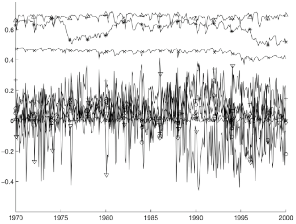
Figure 1.
Normalized topostrophy averaged over the volume of the Arctic Eurasian Basin is plotted for nine AOMIP models [37].
Figure 1.
Normalized topostrophy averaged over the volume of the Arctic Eurasian Basin is plotted for nine AOMIP models [37].

The principle result from Figure 1 is that the possible role of entropic forcing, however imperfectly realized in the neptune parameterization, can be quite strong in comparison with the classical forces represented in traditional modeling. At the date of publication (2007), it was not known which trace in Figure 1 might be closer to reality. Subsequently, from a world database of more than 17,000 long term current meter records spanning over 83,000 current meter-months, climatological
was mapped globally as function of latitude and depth [38]. These observations clearly put regionally-averaged Arctic
>+.4. The strong suggestion, as seen also in many cases cited in [33], is that traditional ocean modeling, based upon classical GFD, is systematically deficient.
There is one further note from the current meter observations that may be of special interest to readers of Entropy. Globally
is positive with overall mean value near +.3 (based on available data). It has long been understood in classical GFD that mean flows, under the influence of background rotation, tend to follow contours of bottom topography. Hence f x u tends to align with ∇D. But either sign for f x u·∇D is allowed. Why does observed
so clearly favour positive sign? As we’ve seen, entropic forcing introduces the Second Law (2), supplying classical GFD with an “Arrow of Time”, thereby selecting the sign of
.
Three more recent publications should be mentioned. [39] examined topostrophy among four global ocean models: two with relatively coarse grid spacing, two with finer grid spacing. None of the four employed neptune. The two models with finer grids tended to produce somewhat more positive topostrophy.
[40] explored introducing neptune into a global model with sufficiently fine grid that the model spontaneously generated eddies (albeit poorly resolved). In such models it is usual to replace Laplacian friction with a biharmonic form (i.e., ∇2 with ∇4). Correspondingly, neptune was represented as A∇4(u−u*). The interesting question is: if realized eddies are already generating entropy, what role is left for an entropy generation parameterization? Comparing model runs with and without u*, [40] obtained modest improvements with u* present, suggesting that explicit eddy generation was not fully represented.
Finally, returning to the Arctic, the model “OPA-LIM” [41,42], not previously included in AOMIP studies, was examined [43]. Consistently with prior AOMIP results, cf. Figure 1, markedly higher
was found [43] when OPA-LIM was modified for neptune. This study also allowed detailed examination of entropically forced cyclonic “rim currents”.
5.2 Differential Mixing of Heat and Salt in the Ocean
We turn to a very different example on very different scales in order to see how robust are some of the entropic insights. The example is chosen because it illustrates another circumstance where simpler intuition has led to mistaken ideas, and entropic calculus reveals surprising understandings with practical, observable consequences.
We contemplate mixing heat and salt by small scale turbulence in the gravitationally stably stratified ocean. Larger scale motions are regarded as internal gravity waves. Occasional superpositions of waves yield local regions of instability (“breaking”) where turbulent mixing occurs. Energy is stored both as kinetic energy and as gravitational potential energy, with spectral densities U(k) and B(k) respectively. Here we will treat k merely as magnitude wavenumber. In fact, motions on larger scales are quite anisotropic, and one should at least distinguish vertical and horizontal wavenumbers. At smaller scales, even during more intense turbulent events, anisotropy tends to persist. This is a complication to which the reader should be aware, but which will not overly concern us for the present level of discussion. Potential energy arises because heat and salt affect the density of sea water due to volumetric coefficients of thermal expansion and haline contraction. It is convenient to define buoyancy, b(x,t) = ρ0(z,t)−ρ(x,t), where ρ is density and ρ0 is regionally horizontally averaged ρ. Gravitational potential energy occurs due to fluctuations in b such that specific potential energy (per unit mass) is B = ½gZb2/ρ02 where g is the acceleration of gravity and Z= (∂zlogρ0)-1 is a height scale due to stable background stratification in ρ0. Specific kinetic energy is U = ½u·u. Spectral energy balance equations for B and U are:
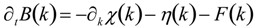 and:
and:
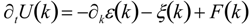 where χ(k) is transfer (by nonlinear effects) of B from wavenumbers less than k to wavenumbers greater than k, ε(k) is the corresponding transfer of U, η(k) is the dissipation of B due to thermal and haline conduction, and ξ(k) is the dissipation of U due to viscosity. Importantly, F is an exchange of energy between B and U by vertical buoyancy flux, F = gwb/ρ0, due to correlations of vertical velocity, w, with b.
Traditional understanding has characterized large scale motion as interaction among waves until, at some smaller scale, waves “break” and turbulence ensues. At the scales of wavelike motion, F should vanish on average since individual waves carry no mean F and the waves are believed to be nearly in random phase superposition. At the smaller scales of turbulence, we might expect a downward mixing of lighter (more buoyant) water above with denser water below, i.e., F<0. Such downward mixing is necessary to compensate the gradual overall upwelling of deep water that has been supplied by sinking (mainly at high latitudes).
Theoretical approaches are possible. On large scales and assuming waves are sufficiently weak, closure methods described in Section 3 can be applied to waves - turbulence mix. In small amplitude limit, [44] showed that such closures approach the resonant interaction approximation (RIA) seen, e.g., in [45,46]. For RIA, applied to statistically homogenous fields, systematic energy transfers occurs only on triads for which wavevectors k + p + q = 0 and also the intrinsic frequencies of the three wave components must satisfy resonance ωk + ωp + ωq = 0. At larger amplitude, the condition of frequency resonance is somewhat relaxed as near-resonant waves support part of the energy transfer. Finally, in the large amplitude limit, frequency resonance becomes entirely insignificant and all waves participate in energy transfer. Importantly from an entropic view, these closures ranging from RIA to full turbulence strictly satisfy the Second Law (2).
RIA has been explored by [47,48] and others to attempt to account for the observed spectral distribution of oceanic internal wave energy. On the scales for which RIA would be valid, F vanishes. In fact the oceanic scales for which RIA is applicable remain an unresolved question, viz., [49,50]. Closure theories capable of representing strongly interacting waves and turbulence (i.e., beyond RIA) have been examined by [51,52,53,54].
Full examination by closure theory has been to date too daunting, and the above cited works have made partial accounts of the spectral distributions of kinetic or potential or wave energy. Vertical buoyancy flux F was considered [53] but only under the very restrictive and unrealistic constraint of motion confined to a vertical plane. Let us here see how the concept of entropy gradient forcing, C·∂YH in (6), can help us foresee the more complete picture despite specific uncertainties that will remain for closure theory and/or numerical experimentation.
In equations (18) for ∂t(B,U) we seek to represent terms arising from C∂H/∂(B,U) where ∂H is change of total entropy with respect to changes ∂(B,U) in B and U while C is an operator projecting these entropy tendencies onto ∂t(B,U). Here, although scales of motion are very much closer to scales of molecular chaos (compared with Section 5.1), we can still proceed without taking direct account of molecular contributions to H [included parametrically as η and ξ in (18)].
Omitting external forcing and internal dissipation, dynamics conserve the total energy, B+U. ME thus favours energy equipartition. This is far from reality in which large scale forcing and small scale dissipation lead to spectra steeply decreasing with increasing wavenumber k. The result is a strongly entropically driven forward transfer of both B and U from small k toward large k. Traditional scaling arguments from turbulence are not so directly applicable due to additional parameters that have entered on account of gravitationally stable background stratification, cf. [55,56,57,58,59].
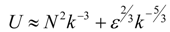
At small scales (large k), one might imagine approaching classical (unstratified) turbulence. For the moment we consider B and U. Later we return to F. B and U behave similarly on scales for which turbulent advection dominates both. Writing for U, nonlinear transfer:
 where U* is constant over modes. Operator K is sometimes hypothesized as a sort of diffusion, K≈∂kDU∂k, with k-dependent coefficient DU. With (19), this suggests ε ≈ − DU∂kU. Continuing for this moment with classical turbulence ideas, if we hypothesize that DU depends only upon “local” scale k and ε(k), we must take DU ≈ ε1/3k8/3 ≡ τ-1k-2/3, where an “eddy timescale” is

Then:
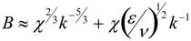
 a classical result since Kolmogorov [60], albeit argued differently by different authors. Considerations for B are similar to those for U on scales for which advection dominates, hence B ≈ χ2/3k-5/3 on scales for which η and ξ in (18) are not important while we continue, for this moment, to set aside F. Further considerations arise because the ratio of viscosity, v, to thermal conductivity, κ, is near v∕κ ≈ 7 while the ratio of viscosity to haline conductivity, γ, is near v∕γ ≈ 700 for seawater. Thus, fluctuations in temperature or salinity persist to smaller scales (larger k) where velocity fluctutations are suppressed by viscosity. On these scales, k > kK where kK =(ε∕v3)1/4, Batchelor [61] argued that the eddy timescale should be given by a characteristic straining rate (ε∕v)1/2 due to velocity fluctuations near k ≈ kK, yielding B ≈ χ(ε∕v)1/2k-1. Over the broader range of scales including k < kK, this yields:
 neglecting so far the role of stable stratification.
A reader may feel alarmed in the previous paragraph for the many uses of “≈” and other “loose” arguments. While this is due in part to necessary brevity in the present paper (more complete discussion having filled literature for decades), it is appropriate to recognize that further careful work remains. Only for present purpose the preceding “thumbnail” may capture some of classical turbulence theory sufficiently to let us proceed. Notably for readers of Entropy, we see that these “cascades” of B and U are driven by entropy generation, ultimately expressed at the level of molecular chaos.
At some sufficiently large scale (small k), it may be that RIA describes wave-wave energy transfers, viz. [47,48]. While neither the RIA limit nor the turbulent limit may be fully realized in the ocean, a greater challenge yet is to bridge the intermediate scales with mixed wavelike and turbulent-like properties. In closure theory a crucial quantity is termed “triple correlation timescale”, θk,p,q, characterizing the time over which three modes satisfying k+p+q=0 can remain phase-correlated to enable systematic energy transfers. A bridge between wave interactions and turbulence was seen [44] where:
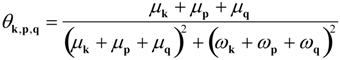 limits on πδ(ωk + ωp + ωq) in a weak wave limit, μ ∕ ω → 0, and upon (μk + μp + μq)-1 in a turbulence limit, ω ∕ μ → 0, where μ is a nonlinear deformation rate obtained from the closure theory. It is this full evaluation from closure theory that has, to date, remained daunting.
We can push a little ahead with some simplifying, albeit uncertain, suppositions. If we suppose the energy transfers ε and χ are only weakly divergent in k on scales for which dissipation rates η and μ are small, i.e., supposing that buoyancy flux F does not dominate, then we may associate μ(k) ≈ τ-1(k) with as (20). At intermediate scales, between weak waves and strong turbulence, we suppose precise resonances ωk + ωp + ωq ≅ 0 are not crucial and estimate for typical triples of waves (ωk + ωp + ωq)2 is “roughly” N2 where N is termed “buoyancy frequency”, N2 = −g∂zlogρ0. Near a scale k, we estimate (23) simply as θ ≈ τ-2∕(τ-2 + N2). From closure theories we know energy transfers are proportional to θ. Thus, if we appeal to the simple heuristic ε ≈ −DU∙∂kU, then take DU∙ ≈ θτ-2k2 which, with the expression for θ, yields:
 and similarly:
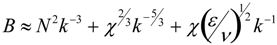 apart from the direct roles of dissipation at high k and the effects of near-resonances for wavelike interactions at low k. Spectra near (24) are observed in oceans [62] and in the middle atmosphere [63].
For clarity of illustration, Figure 2a shows k2U, k2BT and k2BS, where we assume (for reasons to be explained shortly) that total buoyancy, B, is contributed in a representative oceanic example 60% from temperature fluctuations yielding BT and 40% from salinity (concentration of dissolved ions) fluctuations yielding BS.
In obtaining (24), we’ve not especially depended upon entropic forcing ideas. We see “forward” (i.e., from large scales or low k to small scales or high k) energy transfers, ε > 0 and χ > 0, driven by the relative excess of energy at large scales compared with small scales (i.e., far from ME). The different dependences upon k in the terms in (24) reflect different processes that affect the efficiencies of transfers. Significantly, we know [15] that closure theories which lead to (24) are proven to satisfy (2). Nonetheless, we could have inferred these spectra without considering entropy.
The subject turns unexpected, indeed startling, when we inquire about F. Recall that traditional thinking supposes F ≈ 0 on larger, more wavelike scales with F < 0 (i.e., downgradient buoyancy mixing) on smaller, more turbulent scales. Turbulence is usually thought to occur on scales for which density structures are occasionally overturned, observed to occur near a scale kb = (N3∕ε)1/2 where spectra (24) turn from k-3 to k-5/3. Efforts to observe downgradient F have been frustrating. Laboratory experiments [64,65,66] and numerical simulations [67,68,69] often suggest just the opposite, F > 0, termed “persistent countergradient fluxes”. Why?
A tendency toward energy equipartition (here ME) occurs not only across scales of k but also among the available modes of motion at any k. Linear modes from (4), assuming incompressibility, ∇∙u = 0, include two inertio-gravity waves (oppositely propagating) and a geostrophic mode (sometimes called “vortical”) mode. When these three are equally excited, then U = 2B at each k [70]. A reader might also intuit this by realizing that only two components of u are independent, given ∇∙u = 0, while a third variable is b, so that energy is shared among two velocity components and one buoyancy component at each k.
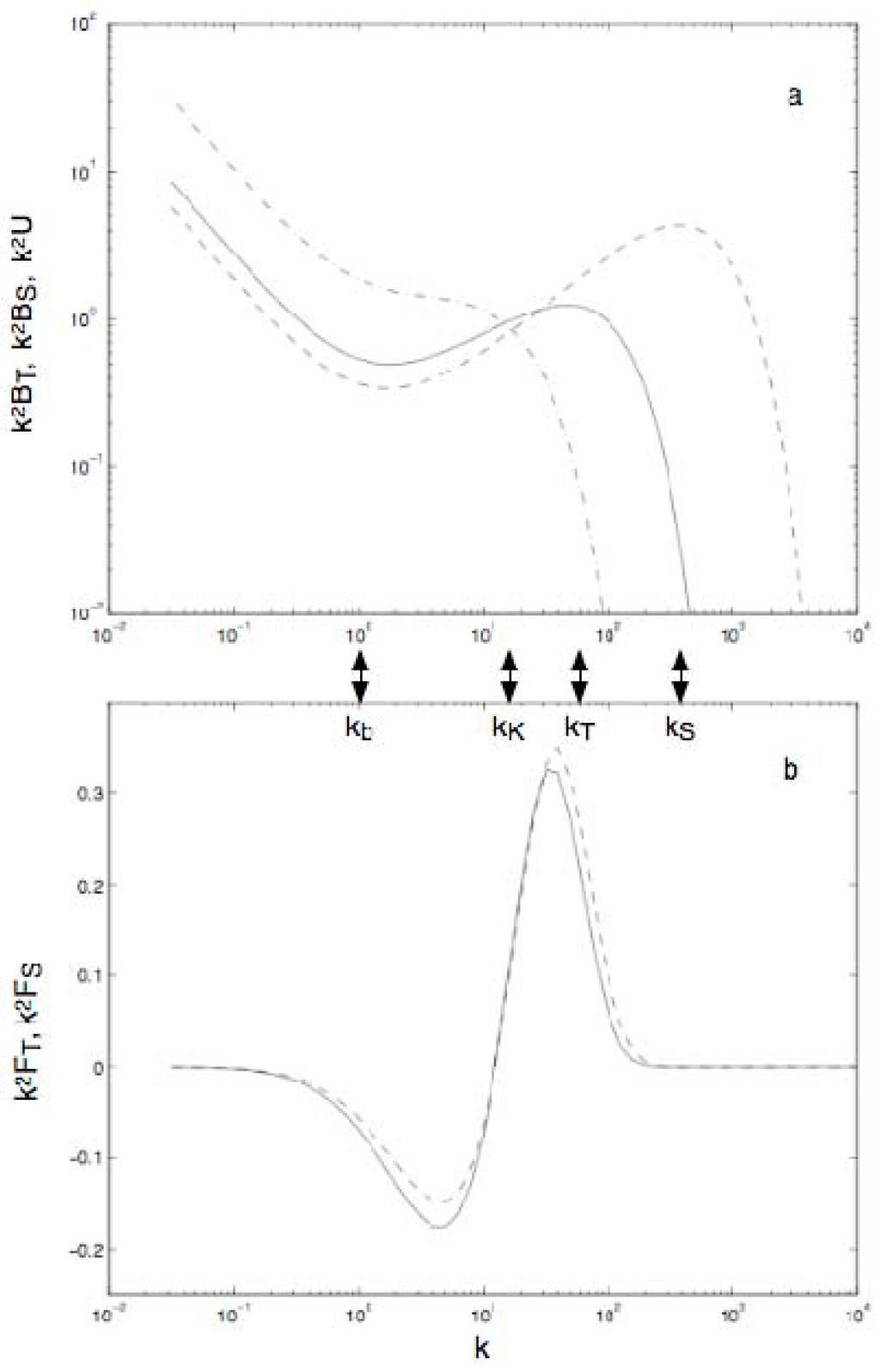
Figure 2.
(a) Spectra k2BT (solid line), k2BS (dashed line) and k2U (dash-dot) are shown. (b) Spectra k2FT (solid line) and k2FS (dashed line) are shown where FT and FS are contributions to total buoyancy flux F=w’b’ due to temperature, T, and salinity, S. Scalings are assumed such that buoyancy wavenumber kb=1 while Kolmogorov kK and diffusive cutoffs kT and kS for T and S are representative of corresponding typical oceanic values.

There develops a competition between entropy generating processes. On one hand, excess energy (both U and B) at low k drive positive transfers ε and χ. But the transfers are not equally efficient. Even in the absence of gravitationally stable stratification, it is well known from closure theories (viz., [71]) that transfer of tracer variance, here b2, is more efficient than transfer of velocity variance, u∙u. The result is to retain somewhat more kinetic energy, U, in the sense U > 2B at low k while accumulating somewhat more potential energy, B, in the sense 2B > U at high k. Then F arises as the entropic forcing, C∙∂YH, at each local k driving toward U = 2B. At lower k, |F| will be impeded by wave propagation tendencies.
Quantifying details of F will require closure theoretic investigation beyond present scope, including taking account of anisotropy of B and U. With plausible assumptions, [72] obtained F as seen in Figure 2b. Again for clarity the figure shows k2FT and k2FS where FT and FS are contributions from T and S in the representative oceanic case shown in Figure 2a. The choice to weight by k2 allows one to better see the countergradient fluxes F < 0.
Details of this F are uncertain. We cannot say, e.g., at precisely what k the sign of F changes from F < 0 at lower k to F > 0 at higher k, and we do not know how effectively wave propagation suppresses |F| at yet lower k [73]. What is stunning though is how strongly this theoretical result contradicts traditional thinking. We anticipate F < 0 over scales for which it was supposed F ≈ 0. We anticipate F > 0 over scales for which it was supposed F < 0. Thus “turbulence”, over k > kb is not expending kinetic energy to mix buoyancy downward but rather the turbulence is being excited by release of potential energy as buoyancy “re-stratifies” (upwards flux). Is all of this very strange? No. F is only taking the sign of positive entropy production, i.e., following the Arrow of Time.
With such clear contrast between present theory and traditional thinking, can the difference be tested? It’s not easy. Although laboratory experiments and numerical simulations have shown persistent countergradient fluxes, F>0, there are always questions how any experiment (laboratory or numerical) is set up. Interestingly, the oceans offer another test, possibly with greater consequences.
As mentioned at Figure 2a, we illustrate for the case of buoyancy in seawater which is controlled by both temperature, T, and salinity, S. However the molecular coefficient, κT, for thermal conduction is about 100x greater than the coefficient, κS, for ionic conduction. There are regions of the ocean which may be gravitationally stably stratified with respect to one tracer while unstably stratified with respect to the other tracer while the total density remains stable, ∂zρ0 < 0. This leads to many interesting phenomena, generally termed “double diffusive”. Throughout much of the oceans, stratification is stable with respect to both T and S, i.e., ∂zT > 0 and ∂zS < 0. Then the usual practice supposes that turbulent mixing is the same for T and S in the sense that vertical fluxes w’T’ and w’S’ are represented by the same eddy diffusion coefficients, AT and AS. I.e., γ ≡ AS/AT = 1.
If traditional views about turbulent mixing in stably stratified flows were correct, we would expect small scale turbulence to support downgradient fluxes. The lesser molecular conduction coefficient, κS, would allow a somewhat wider range of downgradient flux, w’S’, hence γ < 1. On the other hand, if the arguments for F from entropic forcing are correct, then we expect small scale turbulence to be characterized by countergradient (upgradient) w’T’ and w’S’ which will be partially offsetting downgradient fluxes from larger scales. In this case a somewhat wider range for w’S’ permits somewhat greater offsetting flux for overall γ < 1. Oceanic observations [74], laboratory studies [75], and numerical experiments [69,76] have found γ < 1 in gravitationally stable environments.
6. Outstanding Issues
In all areas of environmental fluid mechanics, from atmospheres to oceans to duck ponds, the number of excited degrees of freedoms enormously exceeds our theoretical and numerical capabilities. Recognizing that dependent variables should be understood as moments over probabilities of all possible configurations of the myriad degrees of freedom for which we retain no explicit knowledge, we anticipate forces acting upon these dependent variables driven by the entropy associated with probabilities for all the missing information. How? That is the quantitative challenge.
Section 5 provides illustrations from two widely disparate aspects of ocean dynamics. In Example 5a we considered how unresolved eddies on scales from km to tens of km provide a mean driving force (neptune) that may organize circulation on the scale of ocean basins. In Example 5b we consider the vertical mixing of heat and salt, with seemingly strange results that the smaller oceanic scales (typically 1 m and smaller) associated with turbulent motion may be supporting counter-gradient fluxes, “unmixing” or restratifiying the ocean. These examples are chosen not only as disparate in scale but also because the results are almost exactly contrary to traditional views which combine the classical mechanics of GFD with intuitive ideas that “turbulence” is a sort of enhanced mixing or friction.
The examples in Section 5 also show inadequacies in research to date. We may feel encouraged that even the rudimentary progress to date already indicates substantial improvement upon otherwise “state of the art”. Doubtless many further exercises, beyond the examples in Section 5, await. However, for the remainder of this paper, let us consider some of the shortcomings and open questions arising in Section 4 and Section 5.
We can ask in what other contexts we understand entropic force, possibly as expressed as C∙∂YH in (6). E.g., entropic elasticity in polymers? Or excluded volume forces in colloids [26]? The relation between entropy gradient formulation and MEP invites further attention. Then the simplifying assumption (7) to render C∙∂YH calculable in terms of K∙(Y*−Y) wants care for identifying Y*, for the (large?) distance│Y*−Y│and for estimating K. Among possible research avenues, some of these issues might be examined within careful closure theoretic calculation such as reviewed in Entropy [12], cf. Section 3.
There is a remark to emphasize at this point. The appearance of Y*, which is itself an ME result, often leads to the mistaken impression one is seeking ME as a model for atmospheres or oceans. Clearly ME is not appropriate for strongly forced, dissipative, open systems like atmospheres and oceans. The theory advanced in this paper is not ME. Rather, what we are doing is using a locus of weak ∂YH (near Y*) as a way to estimate nonzero ∂YH at the actual state Y. Thus the goal is distinctly non-equilibrium rather than ME.
Examples described in Section 5 raise many more specific issues. In the case of neptune (Section 5.1) there is a whole gallery of concerns. First, the idealized dynamics at (8) are far from the more complete dynamics employed in most GCMs. Second, translating
at (14) to u* at (16) depended upon various assumptions the quality of which should be questioned. Third, the choice to represent K = A∇2 is taken more from modeling convenience than sound theory. Seeming improvements to ocean models may be more a reflection upon “state of the art” than upon the basis of neptune schemes (to date!) Nonetheless the evidences of improved modeling are encouraging as early efforts to bring entropic forces into GFD are seen to have such marked consequences.
Guidance for assigning values to parameters is problematic, especially for neptune L2 which takes precise values, α2/α1, in (14) but is uncertain at (16) for practical use in GCMs. Experience to date has led to choices for L ranging from a few km to order of 10 km. This may earn a double negative: it is not unsatisfying. As usual practice takes K = A∇2, the value of A, like L, is a “fudge factor”. From this perspective, the difference between traditional friction and neptune is only that friction assigns (unwittingly and without reason) value L=0 whereas neptune adopts a value that is “not unsatisfying”. We call this progress.
A further aspect of neptune is the vertical transfer of horizontal momentum. Ordinarily this is accomplished by a vertical eddy viscosity term, e.g. ∂z(Av∂zu) with coefficient Av only somewhat larger than vertical diffusion coefficients for T or S. With u* from (16) independent of z, the neptune form for this term remains the same as in traditional modeling. However, the values of Av change enormously. Rather than assuming small scale turbulent momentum mixing, quasigeostrophy in (8) implies that in the ocean interior (away from upper and lower surfaces), we should obtain Av = (f2/N2)Ah where Ah is the horizontal exchange coefficient. Values for Av under neptune are typically some orders of magnitude greater than those used in traditional modeling. Although there has been much experimentation with lateral fluxes, Ah∇2(u−u*), there has been very little testing of ∂z(Av∂zu) with Av = (f2/N2)Ah, and there is no discussion to date about possible impacts on model fidelity.
Over horizontal scales larger than about R = ND/f, hence for most ocean GCMs with grid spacing comparable to, or larger than R, it is appropriate to treat u* as independent of z. However, if one considers features on a scale W, smaller than R, then u* diminishes upwards from bottom topography over a vertical distance approximately fW/N. In this case the vertical exchange term, ∂z(Av∂z(u−u*)), acts to induce vertical shear ∂zu. To this author’s knowledge, such a neptune application has not yet been explored.
There is a further point however. In Section 5.1 we considered neptune with respect to u. Under quasigeostrophy however, u and density, ρ, are linked as f x∂zu = g∇h ρ where ∇h is horizontal gradient. On scales larger than R, neptune forcing toward u* with ∂zu* = 0 implies forcing toward ∇h ρ = 0. In fact forcing toward ocean models adiabatically toward level density surfaces, ∇h ρ = 0, is a popular idea that occurs in models based upon density layers and that was introduced into z-level models [77]. A physical argument for adjusting toward ∇h ρ = 0 is that this is a condition of minimal potential energy. Coincidentally ∇h ρ = 0 corresponds to higher entropy on scales larger than R. But then an interesting quandry may be seen on scales smaller than R. On such scales, entropic consideration suggests ∂zu* ≠ 0, hence ∇h ρ* ≠ 0 where f x∂zu* = g∇h ρ*. This contradicts popular thinking [77] about potential energy minimization, suggesting instead that an ocean with initially ∇h ρ = 0 would spontaneously build ∇h ρ ≠ 0 on length scales smaller than R, thereby increasing rather than decreasing potential energy. These contradictory predictions have not yet been tested.
Commenting briefly after Section 5.2, perhaps the greatest single shortcoming has been a tendency to treat vaguely defined scale k without more careful analysis of anisotropy. Much stronger closure theoretical calculations as well as high-resolution 3-D numerical experiments will surely guide future research. We find entropic forces leading to a reversal of the sign of buoyancy flux, F, occurring somewhere near kb = (N 3⁄ε)½. Further analyses will be needed to better define k at which F changes sign. Already this is interesting because we find more wave-like disturbances on k ≤ kb supporting the downgradient (F<0) mixing of buoyancy [73] while more turbulent-like k ≥ kb is characterized by countergradient or restratifying F>0. A consequence is that a more diffusive tracer, T, exhibits stronger turbulent transport, w’T’, than does a less diffusive tracer, S.
In this paper, we have used a reduced (or relative) H based upon uncertainty in macroscale variability while ignoring the contribution of molecular chaos, i.e., thermodynamic H. We then attempted to approximate the entropy gradient forcing terms in eq. 6. The present work differs from, and yet complements, efforts [1,2,3] which consider MEP calculations based on thermodynamic H while omitting uncertainty from macroscale variability. Each approach has merit, with MEP strengthened in recent articles [4,6]. We would have both elegance and greater confidence if we could commence from more complete formulation, taking account at once of uncertainty both at molecular level and at macroscale variability.
This paper ends without “Conclusions”. A hope is that theoretical constructs sketched in Section 4 and illustrated with examples in Section 5 can stimulate further research, bringing a statistical mechanical basis to the otherwise classical mechanical understanding of GFD as applied to atmospheres and oceans. And duck ponds.
Acknowledgements
Advice of anonymous reviewers is gratefully acknowledged.
References
- Paltridge, G. W. Global dynamics and climate—A system of minimum entropy exchange. Q. J. R. Meteorol. Soc 1975, 101, 475–484. [Google Scholar] [CrossRef]
- Paltridge, G. W. The steady-state format of global climate. Q. J. R. Meteorol. Soc 1978, 104, 927–945. [Google Scholar] [CrossRef]
- Ozawa, H.; Ohmura, A.; Lorenz, R.D.; Pujol, T. The second law of thermodynamics and the global climate system: a review of the maximum entropy production principle. Rev. Geophys. 2003, 41, 4. [Google Scholar] [CrossRef]
- Dewar, R.C. Information theory explanation of the fluctuation theorem, maximum entropy production and self-organized criticality in non-equilibrium stationary states. J. Phys. A 2003, 36, 631–641. [Google Scholar] [CrossRef]
- Dewar, R.C. Maximum entropy production and non-equilibrium statistical mechanics. In Non-Equilibrium Thermodynamics and Entropy Production: Life, Earth and Beyond; Kleidon, A., Lorenz, R., Eds.; Springer-Verlag: New York, 2005; pp. 41–55. [Google Scholar]
- Dewar, R.C. Maximum entropy production and the fluctuation theorem. J. Phys. A 2005, 38, L371–L381. [Google Scholar] [CrossRef]
- Lorenz, R.D. Full steam ahead – probably. Science 2003, 299, 837–838. [Google Scholar] [CrossRef] [PubMed]
- Salmon, R.; Holloway, G.; Hendershott, M.C. The equilibrium statistical mechanics of simple quasi-geostrophic models. J. Fluid Mech 1976, 75, 691–703. [Google Scholar] [CrossRef]
- Holloway, G. Eddies, waves, circulation and mixing: Statistical geofluid mechanics. Ann. Rev. Fluid Mech. 1986, 18, 91–147. [Google Scholar] [CrossRef]
- Majda, A.J.; Wang, X. Non-Linear Dynamics and Statistical Theories for Basic Geophysical Flows; Cambridge University Press: Cambridge, UK, 2006; p. 551. [Google Scholar]
- Salmon, R. Lectures on Geophysical Fluid Dynamics; Oxford Univ. Press: Oxford, UK, 1998; p. 378. [Google Scholar]
- Frederiksen, J.S.; O’Kane, T. J. Entropy, closures and subgrid modeling. Entropy 2008, 10, 635–683. [Google Scholar] [CrossRef]
- Kraichnan, R. Irreversible statistical mechanics of incompressible hydrodynamic turbulence. Phys. Rev. 1958, 109, 1407. [Google Scholar] [CrossRef]
- Kraichnan, R. H. The structure of isotropic turbulence at very high Reynolds number. J. Fluid Mech. 1959, 5, 497. [Google Scholar] [CrossRef]
- Carnevale, G.; Frisch, U.; Salmon, R. H theorems in statistical fluid dynamics. J. Phys. A: Math. Gen. 1981, 14, 1701. [Google Scholar] [CrossRef]
- Frederiksen, J. Subgrid-scale parameterizations of eddy-topographic force, eddy viscosity, and stochastic backscatter for flow over topography. J. Atmos. Sci. 1999, 56, 1481. [Google Scholar] [CrossRef]
- Frederiksen, J.; O’Kane, T. Inhomogeneous closure and statistical mechanics for Rossby wave turbulence over topography. J. Fluid Mech. 2005, 539, 137–165. [Google Scholar] [CrossRef]
- O’Kane, T.; Frederiksen, J. The QDIA and regularized QDIA closures for inhomogeneous turbulence over topography. J. Fluid Mech. 2004, 504, 133–165. [Google Scholar] [CrossRef]
- O’Kane, T.; Frederiksen, J. Statistical dynamical subgrid-scale parameterizations for geophysical flows. Phys. Scr. 2008, T132, 014033 (11pp). [Google Scholar] [CrossRef]
- Robert, R.; Sommeria, J. Relaxation towards a statistical equilibrium state in two-dimensional perfect fluid dynamics. Phys. Rev. Lett. 1992, 69, 2776–2779. [Google Scholar] [CrossRef] [PubMed]
- Robert, R.; Rosier, C. The modelling of small scales in 2D turbulent flows: A statistical mechanics approach. J. Stat. Phys. 1997, 86, 481–515. [Google Scholar] [CrossRef]
- Kazantsev, E.; Sommeria, J.; Verron, J. Subgridscale eddy parameterization by statistical mechanics in a barotropic ocean model. J. Phys. Oceanogr 1998, 28, 1017–1042. [Google Scholar] [CrossRef]
- Shimokawa, S.; Ozawa, H. Thermodynamics of irreversible transitions in the oceanic general circulation. Geophys. Res. Lett. 2007, 34, L12606. [Google Scholar] [CrossRef]
- Holloway, G. A shelf wave/topographic pump drives mean coastal circulation. Ocean Model. 1986, 68, 12–15. [Google Scholar]
- Onsager, L. Statistical hydrodynamics. Nuovo Cimento Suppl. 2 1949a, 6, 279–287. [Google Scholar] [CrossRef]
- Onsager, L. The effects of shape on the interaction of colloidal particles. Ann. N. Y. Acad. Sci. 1949b, 51, 627–659. [Google Scholar] [CrossRef]
- Holloway, G. Representing topographic stress for large scale ocean models. J. Phys. Oceanogr. 1992, 22, 1033–1046. [Google Scholar] [CrossRef]
- Miller, J. Statistical mechanics of Euler equations in two dimensions. Phys. Rev. Lett. 1990, 65, 2137–2140. [Google Scholar] [CrossRef] [PubMed]
- Robert, R.; Sommeria, J. Statistical equilibrium state in two-dimensional flows. J. Fluid Mech. 1991, 229, 291–310. [Google Scholar] [CrossRef]
- Robert, R.; Rosier, C. The modelling of small scales in 2D turbulent flows: A statistical mechanics approach. J. Stat. Phys 1997, 86, 481–515. [Google Scholar] [CrossRef]
- Alvarez, A.; Tintore, J.; Holloway, G.; Eby, M.; Beckers, J.M. Effect of topographic stress on the circulation in the western Mediterranean. J. Geophys. Res. 1994, 99, 16053–16064. [Google Scholar] [CrossRef]
- Eby, M.; Holloway, G. Sensitivity of a large scale ocean model to a parameterization of topographic stress. J. Phys. Oceanogr. 1994, 24, 2577–2588. [Google Scholar] [CrossRef]
- Holloway, G. From classical to statistical ocean dynamics. Surv. Geophys. 2004, 25, 203–219. [Google Scholar] [CrossRef]
- Polyakov, I. An eddy parameterization based on maximum entropy production with application to modeling of the Arctic Ocean circulation. J. Phys. Oceanogr. 2001, 31, 2255–2270. [Google Scholar] [CrossRef]
- Nazarenko, L.; Holloway, G.; Tausnev, N. Dynamics of transport of ‘Atlantic signature’ in the Arctic Ocean. J. Geophys. Res. 1998, 103, 31003–31015. [Google Scholar] [CrossRef]
- Proshutinsky, A.; Yang, J.; Gerdes, R.; Karcher, M.; Kauker, F.; Hakkinen, S.; Hibler, W.; Holland, D.; Maqueda, M.; Holloway, G.; Hunke, E.; Maslowski, W.; Steele, M.; Zhang, J. Arctic Ocean study: Synthesis of model results and observations. EOS Trans. AGU 2005, 86, 368–371. [Google Scholar] [CrossRef]
- Holloway, G.; Dupont, F.; Goloubeva, E.; Hakkinen, S.; Hunke, E.; Jin, M.; Karcher, M.; Kauker, F.; Maltrud, M.; Morales Maqueda, M.A.; Maslowski, W.; Platov, G.; Stark, D.; Steele, M.; Suzuki, T.; Wang, J.; Zhang, J. Water properties and circulation in Arctic Ocean models. J. Geophys. Res. 2007, 112. [Google Scholar] [CrossRef]
- Holloway, G. Observing global ocean topostrophy. J. Geophys. Res. 2008, 113, C07054. [Google Scholar] [CrossRef]
- Merryfield, Wm.J.; Scott, R. B. Bathymetric influence on mean currents in two high-resolution near-global ocean models. Ocean Model. 2007, 16, 76–94. [Google Scholar] [CrossRef]
- Maltrud, M.; Holloway, G. Implementing biharmonic neptune in a global eddying ocean model. Ocean Model. 2008, 21, 22–34. [Google Scholar] [CrossRef]
- Fichefet, T.; Morales Maqueda, M. A. Sensitivity of a global sea ice model to the treatment of ice thermodynamics and dynamics. J. Geophys. Res. 1997, 102, 12609–12646. [Google Scholar] [CrossRef]
- Madec, G.; Delecluse, P.; Imbard, M.; Levy, C. OPA 8.1 Ocean General Circulation Model Reference Manual. In Notes de l’LPSL.; Universite P. et M. Curie: Paris, France, 1998. [Google Scholar]
- Holloway, G.; Wang, Z. Representing eddy stresses in an Arctic Ocean model. J. Geophys. Res 2009, in press. [Google Scholar] [CrossRef]
- Holloway, G. On the spectral evolution of strongly interacting waves. Geophys. Astrophys. Fluid Dyn. 1979, 11, 271–287. [Google Scholar] [CrossRef]
- Benney, D.J.; Newell, A.C. Random wave closures. Stud. Appl. Math. 1969, 48, 29–43. [Google Scholar]
- Hasselman, K. On the nonlinear energy transfer in a gravity spectrum. J. Fluid Mech. 1962, 12, 481–500. [Google Scholar] [CrossRef]
- McComas, C.H.; Bretherton, F.P. Resonant interaction of oceanic internal waves. J. Geophys. Res. 1977, 83, 1397–1412. [Google Scholar] [CrossRef]
- Olbers, D.J. Nonlinear energy transfer and energy balance of the internal wave field in the deep ocean. J. Fluid Mech. 1976, 74, 375–399. [Google Scholar] [CrossRef]
- Holloway, G. On interaction time scales of oceanic internal waves. J. Phys. Oceanogr. 1982, 12, 293–296. [Google Scholar] [CrossRef]
- McComas, C. H.; Muller, P. Time scales of interaction among oceanic internal waves. J. Phys. Oceanogr. 1981, 11, 139–147. [Google Scholar] [CrossRef]
- Frederiksen, J.S.; Bell, R.C. Statistical dynamics of internal gravity waves—turbulence. Geophys. Astrophys. Fluid Dyn. 1983, 26, 257–301. [Google Scholar] [CrossRef]
- Frederiksen, J.S.; Bell, R.C. Energy and entropy evolution of interacting internal gravity waves and turbulence. Geophys. Astrophys. Fluid Dyn. 1984, 28, 171–203. [Google Scholar] [CrossRef]
- Holloway, G. The buoyancy flux from internal gravity wave breaking. Dyn. Atmos. Oceans 1988, 12, 107–125. [Google Scholar] [CrossRef]
- van Haren, L.; Staquet, C.; Cambon, C. Decaying stratified turbulence: comparison between a two-point closure EDQNM model and direct numerical simulations. Dyn. Atmos. Oceans 1996, 23, 217–233. [Google Scholar] [CrossRef]
- Bolgiano, R. Turbulent spectra in a stably stratified atmosphere. J. Geophys. Res. 1959, 64, 2226–2229. [Google Scholar] [CrossRef]
- Holloway, G. A conjecture relating oceanic internal waves and small scale processes. Atmosphere-Ocean 1983, 21, 107–122. [Google Scholar] [CrossRef]
- Holloway, G. Considerations on the theory of temperature spectra in stably stratified turbulent flows. J. Phys. Oceanogr. 1986, 16, 2179–2183. [Google Scholar] [CrossRef]
- Lumley, J.L. The spectrum of nearly inertial turbulence in a stably stratified fluid. J. Atmos. Sci. 1964, 21, 99–102. [Google Scholar] [CrossRef]
- Weinstock, J. On the theory of temperature spectra in a stably stratified fluid. J. Phys. Oceanogr. 1985, 15, 475–477. [Google Scholar] [CrossRef]
- Kolmogorov, A.N. The local structure of turbulence in an incompressible viscous fluid for very large Reynolds numbers. C. R. Akad. Nauk, SSSR 1941, 30, 301–305. [Google Scholar] [CrossRef]
- Batchelor, G.K. Small scale variation of convected quantities like temperature in a turbulent fluid. J. Fluid Mech. 1959, 5, 113–133. [Google Scholar] [CrossRef]
- Gargett, A.E.; Hendricks, P.J.; Sanford, T.B.; Osborn, T.R.; Williams, A.J., III. A composite spectrum of vertical shear in the upper ocean. J. Phys. Ocean. 1981, 11, 1258–1271. [Google Scholar] [CrossRef]
- Dewan, E.M.; Good, R.E. Saturation and the ‘‘universal’’ spectrum for vertical profiles of horizontal scalar winds in the atmosphere. J. Geophys. Res. 1986, 91, 2742–2748. [Google Scholar] [CrossRef]
- Itsweire, E.C.; Helland, K.N.; van Atta, C.W. The evolution of grid-generated turbulence in a stably stratified fluid. J. Fluid Mech. 1986, 162, 299–338. [Google Scholar] [CrossRef]
- Komori, S.; Nagata, K. Effects of molecular diffusivities on countergradient scalar and momentum transfer in strongly stable stratification. J. Fluid Mech. 1996, 326, 205–237. [Google Scholar] [CrossRef]
- Stillinger, D.C.; Helland, K.N.; Van Atta, C.W. Experiments on the transition in a stably stratified shear flow. J. Fluid Mech. 1983, 131, 91–122. [Google Scholar] [CrossRef]
- Gargett, A.E.; Merryfield, W.J.; Holloway, G. Direct numerical simulation of differential scalar diffusion in three-dimensional stratified turbulence. J. Phys. Ocean. 2003, 33, 1758–1782. [Google Scholar] [CrossRef]
- Merryfield, W.J.; Holloway, G.; Gargett, A.E. Differential vertical transport of heat and salt by weak stratified turbulence. Geophys. Res. Lett. 1998, 25, 2773–2776. [Google Scholar] [CrossRef]
- Merryfield, W.J. Dependence of differential mixing on N and R_rho. J. Phys. Ocean. 2005, 991–1003. [Google Scholar] [CrossRef]
- Waite, M.L.; Bartello, P. Stratified turbulence dominated by vortical motion. J. Fluid Mech. 2004, 517, 281–308. [Google Scholar] [CrossRef]
- Lesieur, M. Turbulence in Fluids; Martin Nijhoff Publishers: Dordrecht, The Netherlands, 1987; p. 286. [Google Scholar]
- Holloway, G. Statistically stationary differential diffusion in a large-scale internal waves–vortical modes environment. Deep-Sea Res. II 2006, 53, 116–127. [Google Scholar] [CrossRef]
- Sidi, C.; Dalaudier, F. Temperature and heat flux spectra in the turbulent buoyancy subrange. Pure Appl. Geophys. 1989, 130, 547–569. [Google Scholar] [CrossRef]
- Nash, J.D.; Moum, J.N. Microstructure estimates of turbulent salinity flux and the dissipation spectrum of salinity. J. Phys. Ocean. 2002, 32, 2312–2333. [Google Scholar] [CrossRef]
- Jackson, P.R.; Rehmann, C.R. Laboratory measurements of differential diffusion in a diffusively stable, turbulent flow. J. Phys. Ocean. 2003, 33, 1592–1603. [Google Scholar] [CrossRef]
- Smyth, W.D.; Nash, J.D.; Moum, J.N. Differential diffusion in breaking Kelvin–Helmholtz billows. J. Phys. Ocean. 2005, 35, 1004–1022. [Google Scholar] [CrossRef]
- Gent, P. R.; McWilliams, J.C. Isopycnal mixing in ocean circulation models. J. Phys. Oceanogr 1990, 20, 150–155. [Google Scholar] [CrossRef]
© 2009 by the authors; licensee Molecular Diversity Preservation International, Basel, Switzerland. This article is an open-access article distributed under the terms and conditions of the Creative Commons Attribution license (http://creativecommons.org/licenses/by/3.0/).