Solvability of a State–Dependence Functional Integro-Differential Inclusion with Delay Nonlocal Condition

Abstract

There is great focus on phenomena that depend on their past history or their past state. The mathematical models of these phenomena can be described by differential equations of a self-referred type. This paper is devoted to studying the solvability of a state-dependent integro-differential inclusion. The existence and uniqueness of solutions to a state-dependent functional integro-differential inclusion with delay nonlocal condition is studied. We, moreover, conclude the existence of solutions to the problem with the integral condition and the infinite-point boundary one. Some properties of the solutions are given. Finally, two examples illustrating the main result are presented.

1. Introduction

A functional equation is an equation involving an unknown function at more than an argument value. In functional equations, argument deviations are the variations between the argument values of an unknown function and an independent variable t. The functional differential equation, or differential equations with diverging arguments, is created by combining the concepts of differential and functional equations. Functional differential equations are used to describe many phenomena in different sciences, see [1]. Nonlocal problems in mathematical physics are problems in which, unlike traditional boundary value conditions, the desired function’s values at distinct places of the boundary (and/or its values at the boundary and outside it) are related. In fact, it is reasonable to treat the theory of functional differential equations and the theory of nonlocal problems as one indivisible theory.

For various reasons, many researchers have been interested in researching the nonlocal problem of functional differential equations with infinite point conditions; see for example [2,3,4,5,6,7,8,9,10]. The deviation of the argument in the current literature’s differential and integral equations with diverging arguments usually concerns only the time itself, see [11,12]. In theory and practice, however, another case exists in which the deviating arguments are dependent on both the state variable y and the time t. Several studies devoted to such differential equations have lately been published, for example [13,14,15,16,17]. The first papers studying this class of functional equations with self-reference, Eder [18], studied the existence of the unique solution for the differential equation

$$z^{\prime }\left(t\right)=z\left(z\left(t\right)\right),z\left(0\right)=z_0,t\in B\subset \mathbb{R}.$$

Wang [19] studied the strong solution and maximal strong solution for the equation

$$z^{\prime }\left(t\right)=h\left(z\left(z\left(t\right)\right)\right),$$

where $h:\mathbb{R}\to \mathbb{R}$ is continuous and monotone, and $h\left(0\right)=0$.

Feckan [20] studied the existence solution

$$z^{\prime }\left(t\right)=h\left(z\left(z\left(t\right)\right)\right),z\left(0\right)=0whereh\in C^1(\mathbb{R},\mathbb{R}).$$

Buica [13] studied the existence and continuous dependence of solutions, on $z_0$ of the functional differential equation

$$z^{\prime }\left(t\right)=h(t,z\left(z\left(t\right)\right)),z\left(t_0\right)=z_0,t\in [a,b],$$

where $t_0,x_0\in [a,b]$ and $h\in C\left(\right[a,b],[a,b\left]\right)$.

Stanek [21] studied global properties of decreasing solution of the equation

$$z^{\prime }\left(t\right)=z\left(z\left(t\right)\right)+z\left(t\right).$$

Stanek [16] studied global properties of solution of the functional differential equation

$$z\left(t\right)z^{\prime }\left(t\right)=kz\left(z\left(t\right)\right)0<\left|k\right|<1.$$

In this study, the initial value problem of the functional differential inclusion with self-dependence on a nonlinear delay integral operator

$$\frac{\mathrm{d}y}{\mathrm{d}t}\in \mathrm{\Psi }\left(t,y\left({\int }_0^{\mu \left(t\right)}\psi (u,y\left(u\right))\mathrm{d}u\right)\right)a.e.t\in (0,B],$$

(1)

with the nonlocal condition

$$y\left(0\right)+\sum _{\ell =1}^{\kappa }{q}_{\ell }y\left(\mu \left({\tau }_{\ell }\right)\right)=y_0,q_{\ell }>0,{\tau }_{\ell }\in (0,B),$$

(2)

was investigated. We study the existence of the absolutely continuous solution $y\in AC[0,B]$ and demonstrate the continuous dependence on $y_0$ and $\psi$. Moreover, as applications, we study the nonlocal problem of Equation (1) with the integral condition

$$y\left(0\right)+{\int }_0^{B}y\left(\mu \left(u\right)\right)\mathrm{d}h\left(u\right)=y_0,h:[0,B]\to \mathbb{R}(\mathrm{increasing}\mathrm{function})$$

(3)

and with the infinite-point boundary condition

$$y\left(0\right)+\sum _{\ell =1}^{\infty }{q}_{\ell }y\left(\mu \left({\tau }_{\ell }\right)\right)=y_0,$$

(4)

if ${\sum }_{\ell =1}^{\infty }{q}_{\ell }$ is convergent.

The paper is organized as follows: In Section 2, the equivalence of the functional differential inclusion with state-dependence on the nonlinear delay integral operator (1) with the nonlocal condition (2) is given. In Section 3, we study the existence of absolutely continuous solutions to problem (1) and (2), and conclude the existence of solutions to problem (1) with the integral condition (3) and the infinite-point boundary condition (4). In Section 4, we establish the existence of exactly one solution for (1) and (2). In Section 5, the continuous dependence of the solution is studied. Finally, in Section 6, two examples are given to corroborate the main existence result and a numerical example is given to demonstrate the difference between the exact solution and numerical solution.

2. Auxiliary Results

Consider the following assumptions:

(a)

$\mathrm{\Psi }(t,y)$ is nonempty, convex and closed $\forall (t,y)\in [0,B]\times \mathbb{R}$.

(b)

$\mathrm{\Psi }(t,y)$ is measurable in $t\in [0,B]$ for every $y\in \mathbb{R}$.

(c)

$\mathrm{\Psi }(t,y)$ is upper semi continuous in y for every $t\in [0,B]$.

(d)

There exist a bounded measurable function $c:[0,B]\to \mathbb{R}$ and a positive constant b, such that

$$\parallel \mathrm{\Psi }(t,y)\parallel =sup\left\{\left|r\right|:r\in \mathrm{\Psi }(t,y)\right\}\le \left|c\left(t\right)\right|+b\left|y\right|,\left|c\left(t\right)\right|\le M.$$

From the assumptions (a)–(d), we can deduce that there exists a $r\in \mathrm{\Psi }(t,y)$, such that the following is satisfied:

(1)

$r:[0,B]\times \mathbb{R}\to \mathbb{R}$ satisfies Carathéodory condition:

-

For each $t\in [0,B],r(t,.)$ is continuous;

-

For each $\varrho \in \mathbb{R},r(.,\varrho )$ is measurable;

-

There exist a bounded measurable function $c\left(t\right)$ and a positive constant $b>0$, such that

$$\left|r\right(t,\varrho \left)\right|\le \left|c\right(t\left)\right|+b\left|\varrho \right|,\left|c\right(t\left)\right|\le M.$$

and the functional r satisfies the integro-differential equation

$$\frac{\mathrm{d}y}{\mathrm{d}t}=r\left(t,y\left({\int }_0^{\mu \left(t\right)}\psi (u,y\left(u\right))\mathrm{d}u\right)\right)a.e.t\in (0,B],$$

(5)

(2)

$\psi :[0,B]\times \mathbb{R}\to {\mathbb{R}}^{+}$ satisfies Carathéodory condition:

-

For each $t\in [0,B],$$\psi (t,.)$ is continuous;

-

For each $y\in \mathbb{R},$$\psi (.,y)$ is measurable;

-

$\left|\psi \right(t,y\left)\right|\le 1.$

(3)

$\mu :[0,B]\to [0,B]$ is continuous and nondecreasing, $\mu \left(t\right)\le t,t\in [0,B]$.

(4)

$\left(1+2{\sum }_{\ell =1}^{\kappa }{q}_{\ell }\right)bB<1.$

Remark 1.

From $\left(a\right)$ and $\left(1\right),$ we can deduce that every solution of (1) is also a solution of (5).

The equivalence of (5)–(2) and the integral equation is given in the following lemma.

Lemma 1.

If $\left(1\right)$–$\left(4\right)$ hold, then the nonlocal problem (1) and (2) and the equation

$$\begin{array}{ccc}\hfill y\left(t\right)& =& \frac{1}{1+{\sum }_{\ell =1}^{\kappa }{q}_{\ell }}\left[y_0-\sum _{\ell =1}^{\kappa }{q}_{\ell }{\int }_0^{\mu \left({\tau }_{\ell }\right)}r\left(u,y\left({\int }_0^{\mu \left(u\right)}\psi \left(\varrho ,y\left(\varrho \right)\right)\mathrm{d}\varrho \right)\right)\mathrm{d}u\right]\hfill \\ & & +{\int }_0^{t}r\left(u,y\left({\int }_0^{\mu \left(u\right)}\psi (\varrho ,y\left(\varrho \right))\mathrm{d}\varrho \right)\right)\mathrm{d}u\mathrm{for}t\in [0,B]\hfill \end{array}$$

(6)

are equivalent.

Proof. 

Assume that the solution of the nonlocal problem (1) and (2) exists. Integrating (5) from 0 to t, we get

$$y\left(t\right)=y\left(0\right)+{\int }_0^{t}r\left(u,y\left({\int }_0^{\mu \left(u\right)}\psi \left(\varrho ,y\left(\varrho \right)\right)\mathrm{d}\varrho \right)\right)\mathrm{d}u.$$

(7)

Using the condition (2), we obtain

$$\sum _{\ell =1}^{\kappa }{q}_{\ell }y\left(\mu \left({\tau }_{\ell }\right)\right)=y\left(0\right)\sum _{\ell =1}^{\kappa }{q}_{\ell }+\sum _{\ell =1}^{\kappa }{q}_{\ell }{\int }_0^{\mu \left({\tau }_{\ell }\right)}r\left(u,y\left({\int }_0^{\mu \left(u\right)}\psi (\varrho ,y\left(\varrho \right))\mathrm{d}\varrho \right)\right)\mathrm{d}u.$$

By ${\sum }_{\ell =1}^{\kappa }{q}_{\ell }y\left(\mu \left({\tau }_{\ell }\right)\right)=y_0-y\left(0\right)$, we have

$$y_0-y\left(0\right)=y\left(0\right)\sum _{\ell =1}^{\kappa }{q}_{\ell }+\sum _{\ell =1}^{\kappa }{q}_{\ell }{\int }_0^{\mu \left({\tau }_{\ell }\right)}r\left(u,y\left({\int }_0^{\mu \left(u\right)}\psi (\varrho ,y\left(\varrho \right))\mathrm{d}\varrho \right)\right)\mathrm{d}u,$$

which implies

$$y\left(0\right)=\frac{1}{1+{\sum }_{\ell =1}^{\kappa }{q}_{\ell }}\left[y_0-\sum _{\ell =1}^{\kappa }{q}_{\ell }{\int }_0^{\mu \left({\tau }_{\ell }\right)}r\left(u,y\left({\int }_0^{\mu \left(u\right)}\psi (\varrho ,y\left(\varrho \right))\mathrm{d}\varrho \right)\right)\mathrm{d}u\right].$$

(8)

Using (7) and (8), we obtain

$$\begin{array}{ccc}\hfill y\left(t\right)& =& \frac{1}{1+{\sum }_{\ell =1}^{\kappa }{q}_{\ell }}\left[y_0-\sum _{\ell =1}^{\kappa }{q}_{\ell }{\int }_0^{\mu \left({\tau }_{\ell }\right)}r\left(u,y\left({\int }_0^{\mu \left(u\right)}\psi (\varrho ,y\left(\varrho \right))\mathrm{d}\varrho \right)\right)\mathrm{d}u\right]\hfill \\ & & +{\int }_0^{t}r\left(u,y\left({\int }_0^{\mu \left(u\right)}\psi (\varrho ,y\left(\varrho \right))\mathrm{d}\varrho \right)\right)\mathrm{d}u.\hfill \end{array}$$

Now, suppose that $y\in C[0,B]$ is a solution of (6). Now differentiate (6), we arrive at

$$\begin{array}{ccc}\hfill \frac{\mathrm{d}y}{\mathrm{d}t}& =& \frac{\mathrm{d}}{\mathrm{d}t}\left\{\frac{1}{1+{\sum }_{\ell =1}^{\kappa }{q}_{\ell }}\left[y_0-\sum _{\ell =1}^{\kappa }{q}_{\ell }{\int }_0^{\mu \left({\tau }_{\ell }\right)}r\left(u,y\left({\int }_0^{\mu \left(u\right)}\psi (\varrho ,y\left(\varrho \right))\mathrm{d}\varrho \right)\right)\mathrm{d}u\right]\right.\hfill \\ & & \left.+{\int }_0^{t}r\left(u,y\left({\int }_0^{\mu \left(u\right)}\psi (\varrho ,y\left(\varrho \right))\mathrm{d}\varrho \right)\right)\mathrm{d}u\right\}\hfill \\ & =& r\left(t,y\left({\int }_0^{\mu \left(t\right)}\psi (\varrho ,y\left(\varrho \right))\mathrm{d}\varrho \right)\right).\hfill \end{array}$$

From (6), we find

$$\begin{array}{ccc}\hfill y\left({\tau }_{\ell }\right)& =& \frac{1}{1+{\sum }_{\ell =1}^{\kappa }{q}_{\ell }}\left[y_0-\sum _{\ell =1}^{\kappa }{q}_{\ell }{\int }_0^{\mu \left({\tau }_{\ell }\right)}r\left(u,y\left({\int }_0^{\mu \left(u\right)}\psi (\varrho ,y\left(\varrho \right))\mathrm{d}\varrho \right)\right)\mathrm{d}u\right]\hfill \\ & & +{\int }_0^{{\tau }_{\ell }}r\left(u,y\left({\int }_0^{\mu \left(u\right)}\psi (\varrho ,y\left(\varrho \right))\mathrm{d}\varrho \right)\right)\mathrm{d}u,\hfill \end{array}$$

$$y\left(0\right)=\frac{1}{1+{\sum }_{\ell =1}^{\kappa }{q}_{\ell }}\left[y_0-\sum _{\ell =1}^{\kappa }{q}_{\ell }{\int }_0^{\mu \left({\tau }_{\ell }\right)}r\left(u,y\left({\int }_0^{\mu \left(u\right)}\psi (\varrho ,y\left(\varrho \right))\mathrm{d}\varrho \right)\right)\mathrm{d}u\right],$$

(9)

and

$$\begin{array}{ccc}\hfill \sum _{\ell =1}^{\kappa }{q}_{\ell }y\left(\mu \left({\tau }_{\ell }\right)\right)& =& \frac{1}{1+{\sum }_{\ell =1}^{\kappa }{q}_{\ell }}\sum _{\ell =1}^{\kappa }{q}_{\ell }\left[y_0-\sum _{\ell =1}^{\kappa }{q}_{\ell }{\int }_0^{\mu \left({\tau }_{\ell }\right)}r\left(u,y\left({\int }_0^{\mu \left(u\right)}\psi (\varrho ,y\left(\varrho \right))\mathrm{d}\varrho \right)\right)\mathrm{d}u\right]\hfill \\ & & +\sum _{\ell =1}^{\kappa }{q}_{\ell }{\int }_0^{\mu \left({\tau }_{\ell }\right)}r\left(u,y\left({\int }_0^{\mu \left(u\right)}\psi (\varrho ,y\left(\varrho \right))\mathrm{d}\varrho \right)\right)\mathrm{d}u.\hfill \end{array}$$

(10)

From (9) and (10), we have

$$\begin{array}{cc}\hfill & y\left(0\right)+\sum _{\ell =1}^{\kappa }{q}_{\ell }y\left(\mu \left({\tau }_{\ell }\right)\right)=\frac{1}{1+{\sum }_{\ell =1}^{\kappa }{q}_{\ell }}\left(1+\sum _{\ell =1}^{\kappa }{q}_{\ell }\right)\left[y_0-\sum _{\ell =1}^{\kappa }{q}_{\ell }\right.\hfill \\ \hfill & \left.{\int }_0^{\mu \left({\tau }_{\ell }\right)}r\left(u,y\left({\int }_0^{\mu \left(u\right)}\psi (\varrho ,y\left(\varrho \right))\mathrm{d}\varrho \right)\right)\mathrm{d}u\right]\hfill \\ \hfill & +\sum _{\ell =1}^{\kappa }{q}_{\ell }{\int }_0^{\mu \left({\tau }_{\ell }\right)}r\left(u,y\left({\int }_0^{\mu \left(u\right)}\psi (\varrho ,y\left(\varrho \right))\mathrm{d}\varrho \right)\right)\mathrm{d}u.\hfill \end{array}$$

Then

$$y\left(0\right)+\sum _{\ell =1}^{\kappa }{q}_{\ell }y\left(\mu \left({\tau }_{\ell }\right)\right)=y_0.$$

This completes the proof. □

3. Existence of Solution

In the following theorem, using Schauder’s fixed point theorem, we establish the existence of at least one solution of (1) and (2).

Theorem 1.

If $\left(1\right)$–$\left(4\right)$ hold, then the nonlocal problem (1) and (2) has at least one solution $y\in AC[0,B]$.

Proof. 

First, we define the operator A associated with Equation (6) and set $P_L$ by

$$\begin{array}{ccc}\hfill Ay\left(t\right)& =& \frac{1}{1+{\sum }_{\ell =1}^{\kappa }{q}_{\ell }}\left[y_0-\sum _{\ell =1}^{\kappa }{q}_{\ell }{\int }_0^{\mu \left({\tau }_{\ell }\right)}r\left(u,y\left({\int }_0^{\mu \left(u\right)}\psi (\varrho ,y\left(\varrho \right))\mathrm{d}\varrho \right)\right)\mathrm{d}u\right]\hfill \\ & & +{\int }_0^{t}r\left(u,y\left({\int }_0^{\mu \left(u\right)}\psi (\varrho ,y\left(\varrho \right))\mathrm{d}\varrho \right)\right)\mathrm{d}u.\hfill \end{array}$$

Now $P_L=\{y\in C[0,B]:|y\left(t\right)-y\left(u\right)|\le L|t-u|,\forall t,u\in [0,B]\},$ where

$$L=\frac{b|y_0|+(1+{\sum }_{\ell =1}^{\kappa }{q}_{\ell })M}{(1+{\sum }_{\ell =1}^{\kappa }{q}_{\ell })-(1+2{\sum }_{\ell =1}^{\kappa }{q}_{\ell })bB}.$$

Then we have for $y\in P,$

$$\begin{array}{ccc}\hfill \left|Ay\left(t\right)\right|& =& \left|\frac{1}{1+{\sum }_{\ell =1}^{\kappa }{q}_{\ell }}\left[y_0-\sum _{\ell =1}^{\kappa }{q}_{\ell }{\int }_0^{\mu \left({\tau }_{\ell }\right)}r\left(u,y\left({\int }_0^{\mu \left(u\right)}\psi (\varrho ,y\left(\varrho \right))\mathrm{d}\varrho \right)\right)\mathrm{d}u\right]\right.\hfill \\ & & \left.+{\int }_0^{t}r\left(u,y\left({\int }_0^{\mu \left(u\right)}\psi (\varrho ,y\left(\varrho \right))\mathrm{d}\varrho \right)\right)\mathrm{d}u\right|\hfill \\ & \le & \frac{1}{1+{\sum }_{\ell =1}^{\kappa }{q}_{\ell }}\left[|y_0|+\sum _{\ell =1}^{\kappa }{q}_{\ell }{\int }_0^{\mu \left({\tau }_{\ell }\right)}\left|r\left(u,y\left({\int }_0^{\mu \left(u\right)}\psi (\varrho ,y\left(\varrho \right))\mathrm{d}\varrho \right)\right)\right|\mathrm{d}u\right]\hfill \\ & & +{\int }_0^t\left|r\left(u,y\left({\int }_0^{\mu \left(u\right)}\psi (\varrho ,y\left(\varrho \right))\mathrm{d}\varrho \right)\right)\right|\mathrm{d}u,\hfill \end{array}$$

and so

$$\begin{array}{ccc}\hfill \left|Ay\left(t\right)\right|& \le & \frac{1}{1+{\sum }_{\ell =1}^{\kappa }{q}_{\ell }}\left[|y_0|+\sum _{\ell =1}^{\kappa }{q}_{\ell }{\int }_0^{\mu \left({\tau }_{\ell }\right)}\left(\left|c\left(u\right)\right|+b\left|y\left({\int }_0^{\mu \left(u\right)}\psi (\varrho ,y\left(\varrho \right))\mathrm{d}\varrho \right)\right|\right)\mathrm{d}u\right]\hfill \\ & & +{\int }_0^t\left(\left|c\left(u\right)\right|+b\left|y\left({\int }_0^{\mu \left(u\right)}\psi (\varrho ,y\left(\varrho \right))\mathrm{d}\varrho \right)\right|\right)\mathrm{d}u\hfill \\ & \le & \frac{1}{1+{\sum }_{\ell =1}^{\kappa }{q}_{\ell }}\left[|y_0|+\sum _{\ell =1}^{\kappa }{q}_{\ell }{\int }_0^{\mu \left({\tau }_{\ell }\right)}\left(\right|c\left(u\right)|\right.\hfill \\ & & \left.+b\left|y\left({\int }_0^{\mu \left(u\right)}\psi (\varrho ,y\left(\varrho \right))\mathrm{d}\varrho \right)-y\left(0\right)\right|+b\left|y\left(0\right)\right|)\mathrm{d}u\right]\hfill \\ & & +{\int }_0^t\left(\left|c\left(u\right)\right|+b\left|y\left({\int }_0^{\mu \left(u\right)}\psi (\varrho ,y\left(\varrho \right))\mathrm{d}\varrho \right)-y\left(0\right)\right|+b\left|y\left(0\right)\right|\right)\mathrm{d}u.\hfill \end{array}$$

Thus,

$$\begin{array}{ccc}& \le & \frac{1}{1+{\sum }_{\ell =1}^{\kappa }{q}_{\ell }}\left[|y_0|+\sum _{\ell =1}^{\kappa }{q}_{\ell }{\int }_0^{\mu \left({\tau }_{\ell }\right)}\left(\left|c\left(u\right)\right|+bL{\int }_0^{\mu \left(u\right)}\left|\psi (\varrho ,y(\varrho \left)\right)\right|\mathrm{d}\varrho +b\left|y\left(0\right)\right|\right)\mathrm{d}u\right]\hfill \\ & & +{\int }_0^t\left(\left|c\left(u\right)\right|+bL{\int }_0^{\mu \left(u\right)}\left|\psi (\varrho ,y\left(\varrho \right))\right|\mathrm{d}\varrho +b\left|y\left(0\right)\right|\right)\mathrm{d}u\hfill \\ & \le & \frac{1}{1+{\sum }_{\ell =1}^{\kappa }{q}_{\ell }}\left|y_0\right|+\frac{{\sum }_{\ell =1}^{\kappa }{q}_{\ell }}{1+{\sum }_{\ell =1}^{\kappa }{q}_{\ell }}\left(BM+bL{B}^2+bB\left|y\left(0\right)\right|\right)\hfill \\ & & +BM+bL{B}^2+bB\left|y\left(0\right)\right|\hfill \\ & =& \frac{1}{1+{\sum }_{\ell =1}^{\kappa }{q}_{\ell }}\left|y_0\right|+\left(\frac{{\sum }_{\ell =1}^{\kappa }{q}_{\ell }}{1+{\sum }_{\ell =1}^{\kappa }{q}_{\ell }}+1\right)\left(BM+bL{B}^2+bB\left|y\left(0\right)\right|\right).\hfill \end{array}$$

(11)

But

$$\begin{array}{ccc}\hfill \left|y\right(0\left)\right|& =& \left|\frac{1}{1+{\sum }_{\ell =1}^{\kappa }{q}_{\ell }}\left[y_0-\sum _{\ell =1}^{\kappa }{q}_{\ell }{\int }_0^{\mu \left({\tau }_{\ell }\right)}r\left(u,y\left({\int }_0^{\mu \left(u\right)}\psi (\varrho ,y\left(\varrho \right))\mathrm{d}\varrho \right)\right)\mathrm{d}u\right]\right|\hfill \\ & \le & \frac{1}{1+{\sum }_{\ell =1}^{\kappa }{q}_{\ell }}\left[\left|y_0\right|+\sum _{\ell =1}^{\kappa }{q}_{\ell }{\int }_0^{\mu \left({\tau }_{\ell }\right)}\left|r\left(u,y\left({\int }_0^{\mu \left(u\right)}\psi (\varrho ,y\left(\varrho \right))\mathrm{d}\varrho \right)\right)\right|\mathrm{d}u\right]\hfill \end{array}$$

and so

$$\begin{array}{ccc}\hfill \left|y\right(0\left)\right|& \le & \frac{1}{1+{\sum }_{\ell =1}^{\kappa }{q}_{\ell }}\left[|y_0|+\sum _{\ell =1}^{\kappa }{q}_{\ell }{\int }_0^{\mu \left({\tau }_{\ell }\right)}\left(\left|c\right(u\left)\right|\right.\right.\hfill \\ & & \left.\left.+b\left|y\left({\int }_0^{\mu \left(u\right)}\psi (\varrho ,y\left(\varrho \right))\mathrm{d}\varrho \right)-y\left(0\right)\right|+b\left|y\left(0\right)\right|\right)\mathrm{d}u\right]\hfill \\ & \le & \frac{1}{1+{\sum }_{\ell =1}^{\kappa }{q}_{\ell }}\left[|y_0|+\sum _{\ell =1}^{\kappa }{q}_{\ell }{\int }_0^{\mu \left({\tau }_{\ell }\right)}\left(\left|c\left(u\right)\right|+bL{\int }_0^{\mu \left(u\right)}\left|\psi (\varrho ,y\left(\varrho \right))\right|\mathrm{d}\varrho +b\left|y\left(0\right)\right|\right)\mathrm{d}u\right]\hfill \\ & \le & \frac{1}{1+{\sum }_{\ell =1}^{\kappa }{q}_{\ell }}\left[|y_0|+\sum _{\ell =1}^{\kappa }{q}_{\ell }\left(BM+bL{B}^2+bB\left|y\left(0\right)\right|\right)\right].\hfill \end{array}$$

Hence

$$\left|y\left(0\right)\right|\le \frac{|y_0|+(BM+bL{B}^2){\sum }_{\ell =1}^{\kappa }{q}_{\ell }}{\left(1+{\sum }_{\ell =1}^{\kappa }{q}_{\ell }\right)-bB{\sum }_{\ell =1}^{\kappa }{q}_{\ell }}.$$

(12)

From (11) and (12), we obtain

$$\begin{array}{ccc}\hfill \left|Ay\right(t\left)\right|& \le & \frac{1}{1+{\sum }_{\ell =1}^{\kappa }{q}_{\ell }}\left|y_0\right|+\left(\frac{{\sum }_{\ell =1}^{\kappa }{q}_{\ell }}{1+{\sum }_{\ell =1}^{\kappa }{q}_{\ell }}+1\right)\hfill \\ & & \times (BM+bL{B}^2+bB|y\left(0\right)\left|\right)\hfill \\ & \le & \frac{1}{1+{\sum }_{\ell =1}^{\kappa }{q}_{\ell }}\left|y_0\right|+\left(\frac{{\sum }_{\ell =1}^{\kappa }{q}_{\ell }}{1+{\sum }_{\ell =1}^{\kappa }{q}_{\ell }}+1\right)\hfill \\ & & \times \left(BM+bL{B}^2+bB\frac{|y_0|+(BM+bL{B}^2){\sum }_{\ell =1}^{\kappa }{q}_{\ell }}{\left(1+{\sum }_{\ell =1}^{\kappa }{q}_{\ell }\right)-bB{\sum }_{\ell =1}^{\kappa }{q}_{\ell }}\right)\hfill \\ & =& \frac{|y_0|+(BM+bL{B}^2){\sum }_{\ell =1}^{\kappa }{q}_{\ell }}{\left(1+{\sum }_{\ell =1}^{\kappa }{q}_{\ell }\right)-bB{\sum }_{\ell =1}^{\kappa }{q}_{\ell }}+LB.\hfill \end{array}$$

Now, let $t_1,t_2\in (0,B]$ such that $|t_2-t_1|<\delta$, then

$$\begin{array}{ccc}\hfill \left|Ay\left(t_2\right)-Ay\left(t_1\right)\right|& \le & {\int }_{t_1}^{t_2}\left|r\left(u,y\left({\int }_0^{\mu \left(u\right)}\psi (\varrho ,y\left(\varrho \right))\mathrm{d}\varrho \right)\right)\right|\mathrm{d}u\hfill \\ & \le & {\int }_{t_1}^{t_2}\left(\left|c\left(u\right)\right|+b\left|y\left({\int }_0^{\mu \left(u\right)}\psi (\varrho ,y\left(\varrho \right))\mathrm{d}\varrho \right)-y\left(0\right)\right|+b\left|y\left(0\right)\right|\right)\mathrm{d}u\hfill \\ & \le & {\int }_{t_1}^{t_2}\left(\left|c\left(u\right)\right|+bL{\int }_0^{\mu \left(u\right)}\left|\psi (\varrho ,y\left(\varrho \right))\right|\mathrm{d}\varrho +b\left|y\left(0\right)\right|\right)\mathrm{d}u\hfill \\ & \le & (t_2-t_1)M+(t_2-t_1)bLB+(t_2-t_1)b\left|y\left(0\right)\right|\hfill \\ & =& (t_2-t_1)(M+bLB+b|y\left(0\right)\left|\right).\hfill \end{array}$$

(13)

From (12) and (13), we obtain

$$\begin{array}{ccc}\hfill |Ay\left(t_2\right)-Ay\left(t_1\right)|& \le & (t_2-t_1)\left(M+bLB\right.\hfill \\ & & \left.+b\left(\frac{|y_0|+(BM+bL{B}^2){\sum }_{\ell =1}^{\kappa }{q}_{\ell }}{(1+{\sum }_{\ell =1}^{\kappa }{q}_{\ell })-bB{\sum }_{\ell =1}^{\kappa }{q}_{\ell }}\right)\right)\hfill \\ & \le & (t_2-t_1)\frac{b|y_0|+\left(1+{\sum }_{\ell =1}^{\kappa }{q}_{\ell }\right)(M+bLB)}{\left(1+{\sum }_{\ell =1}^{\kappa }{q}_{\ell }\right)-bB{\sum }_{\ell =1}^{\kappa }{q}_{\ell }}=(t_2-t_1)L.\hfill \end{array}$$

This proves that $A:P_L\to P_L$; the class of functions $\left\{Ay\right\}$ is uniformly bounded and equi-continuous in $P_L$.

Let $y_n\in P_L$, $y_n\to y$$(n\to \infty )$, then from assumptions $\left(1\right)$ and $\left(2\right),$ we obtain $r(t,y_n\left(t\right),y_n\left(t\right))\to r(t,y\left(t\right),y\left(t\right))$ and $\psi (t,y_n\left(t\right))\to \psi (t,y\left(t\right))$ as $n\to \infty$. Also

$$\begin{array}{ccc}\hfill \underset{n\to \infty }{lim}A{y}_n\left(t\right)& =& \underset{n\to \infty }{lim}\left(\frac{1}{1+{\sum }_{\ell =1}^{\kappa }{q}_{\ell }}\left[y_0-\sum _{\ell =1}^{\kappa }{q}_{\ell }{\int }_0^{\mu \left({\tau }_{\ell }\right)}r\left(u,y_n\left({\int }_0^{\mu \left(u\right)}\psi (\varrho ,y_n\left(\varrho \right))\mathrm{d}\varrho \right)\right)\mathrm{d}u\right]\right.\hfill \\ & & \left.+{\int }_0^{t}r(u,y_n\left({\int }_0^{\mu \left(u\right)}\psi (\varrho ,y_n\left(\varrho \right))\mathrm{d}\varrho \right))\mathrm{d}u\right).\hfill \end{array}$$

(14)

Now

$$\begin{array}{ccc}& & \left|y_n\left({\int }_0^{\mu \left(u\right)}\psi (\varrho ,y_n\left(\varrho \right))\mathrm{d}\varrho \right)-y\left({\int }_0^{\mu \left(u\right)}\psi (\varrho ,y\left(\varrho \right))\mathrm{d}\varrho \right)\right|\hfill \\ & \le & \left|y_n\left({\int }_0^{\mu \left(u\right)}\psi (\varrho ,y_n\left(\varrho \right))\mathrm{d}\varrho \right)-y_n\left({\int }_0^{\mu \left(u\right)}\psi (\varrho ,y\left(\varrho \right))\mathrm{d}\varrho \right)\right|\hfill \\ & & +\left|y_n\left({\int }_0^{\mu \left(u\right)}\psi (\varrho ,y\left(\varrho \right))\mathrm{d}\varrho \right)-y\left({\int }_0^{\mu \left(u\right)}\psi (\varrho ,y\left(\varrho \right))\mathrm{d}\varrho \right)\right|\hfill \\ & \le & L{\int }_0^{\mu \left(u\right)}\left|\psi (\varrho ,y_n\left(\varrho \right))-\psi (\varrho ,y\left(\varrho \right))\right|\mathrm{d}\varrho +\frac{ϵ}{2}\hfill \\ & \le & \frac{ϵ}{2}+\frac{ϵ}{2}=ϵ.\hfill \end{array}$$

(15)

Using (14) and (15) and Lebesgue’s dominated convergence theorem [22], we obtain

$$\begin{array}{ccc}\hfill \underset{n\to \infty }{lim}A{y}_n\left(t\right)& =& \frac{1}{1+{\sum }_{\ell =1}^{\kappa }{q}_{\ell }}\left[y_0-\sum _{\ell =1}^{\kappa }{q}_{\ell }{\int }_0^{\mu \left({\tau }_{\ell }\right)}\underset{n\to \infty }{lim}r\left(u,y_n\left({\int }_0^{\mu \left(u\right)}\psi (\varrho ,y_n\left(\varrho \right))\mathrm{d}\varrho \right)\right)\mathrm{d}u\right]\hfill \\ & & +{\int }_0^t\underset{n\to \infty }{lim}r\left(u,y_n\left({\int }_0^{\mu \left(u\right)}\psi (\varrho ,y_n\left(\varrho \right))\mathrm{d}\varrho \right)\right)\mathrm{d}u=Ay\left(t\right).\hfill \end{array}$$

Then $A{y}_n\to Ay$ as $n\to \infty$, the operator A is continuous.

Hence by Schauder theorem [23] there exists at least solution $y\in C[0,B]$ for the integral Equation (6), therefore there exists at least solution $y\in AC[0,B]$ for the nonlocal problem (1) and (2). □

• For the nonlocal integral condition, we present the following theorem.

Theorem 2.

If $\left(1\right)$–$\left(4\right)$ hold, then the nonlocal problem of (1), (3) has at least one solution.

Proof. 

Let $y\in AC[0,B]$ be the solution of the nonlocal problem (1) with (3). Let $q_{\ell }=h\left(t_{\ell }\right)-h\left(t_{\ell -1}\right)$, h is an increasing function, ${\tau }_{\ell }\in (t_{\ell -1},t_{\ell })$, $0=t_0<t_1<t_2,\dots <t_{\kappa }=B$ then, as $\kappa \to \infty$ the nonlocal condition (2) will be

$$y\left(0\right)+\sum _{\ell =1}^{\kappa }\left(h\left(t_{\ell }\right)-h\left(t_{\ell -1}\right)\right)y\left(\mu \left({\tau }_{\ell }\right)\right)=y_0$$

and

$$y\left(0\right)+\underset{\kappa \to \infty }{lim}\sum _{\ell =1}^{\kappa }\left(h\left(t_{\ell }\right)-h\left(t_{\ell -1}\right)\right)y\left(\mu \left({\tau }_{\ell }\right)\right)=y\left(0\right)+{\int }_0^{B}y\left(\mu \left(u\right)\right)\mathrm{d}h\left(u\right)=y_0.$$

As $\kappa \to \infty$, the solution of the nonlocal problem (1), (3) will be

$$\begin{array}{ccc}\hfill y\left(t\right)& =& \underset{\kappa \to \infty }{lim}\frac{1}{1+{\sum }_{\ell =1}^{\kappa }{q}_{\ell }}\left[y_0-\sum _{\ell =1}^{\kappa }{q}_{\ell }{\int }_0^{\mu \left({\tau }_{\ell }\right)}r\left(u,y\left({\int }_0^{\mu \left(u\right)}\psi (\varrho ,y\left(\varrho \right))\mathrm{d}\varrho \right)\right)\mathrm{d}u\right]\hfill \\ & & +{\int }_0^{t}r\left(u,y\left({\int }_0^{\mu \left(u\right)}\psi (\varrho ,y\left(\varrho \right))\mathrm{d}\varrho \right)\right)\mathrm{d}u\hfill \\ & =& \frac{1}{1+h\left(B\right)-h\left(0\right)}\left[y_0-\underset{\kappa \to \infty }{lim}\sum _{\ell =1}^{\kappa }{q}_{\ell }{\int }_0^{\mu \left({\tau }_{\ell }\right)}r\left(u,y\left({\int }_0^{\mu \left(u\right)}\psi (\varrho ,y\left(\varrho \right))\mathrm{d}\varrho \right)\right)\mathrm{d}u\right.\hfill \\ & & \left.(h\left(t_{\ell }\right)-h\left(t_{\ell -1}\right))\right]+{\int }_0^{t}r\left(u,y\left({\int }_0^{\mu \left(u\right)}\psi (\varrho ,y\left(\varrho \right))\mathrm{d}\varrho \right)\right)\mathrm{d}u\hfill \\ & =& \frac{1}{1+h\left(B\right)-h\left(0\right)}\left[y_0-{\int }_0^{B}r\left(u,y\left({\int }_0^{\mu \left(u\right)}\psi (\varrho ,y\left(\varrho \right))\mathrm{d}\varrho \right)\right)\mathrm{d}h\left(u\right)\right]\hfill \\ & & +{\int }_0^{t}r\left(u,y\left({\int }_0^{\mu \left(u\right)}\psi (\varrho ,y\left(\varrho \right)\mathrm{d}\varrho \right)\right)\mathrm{d}u.\hfill \end{array}$$

This completes the proof. □

• For the infinite-point boundary condition, we present the following theorem.

Theorem 3.

If $\left(1\right)$–$\left(4\right)$ hold, then the nonlocal problem of (1), (4) has at least one solution.

Proof. 

Let ${\sum }_{\ell =1}^{\kappa }{q}_{\ell }$ be convergent. Then

$$\begin{array}{ccc}\hfill y_{\kappa }\left(t\right)& =& \frac{1}{1+{\sum }_{\ell =1}^{\kappa }{q}_{\ell }}\left[y_0-\sum _{\ell =1}^{\kappa }{q}_{\ell }{\int }_0^{\mu \left({\tau }_{\ell }\right)}r\left(u,y\left({\int }_0^{\mu \left(u\right)}\psi (\varrho ,y\left(\varrho \right))\mathrm{d}\varrho \right)\right)\mathrm{d}u\right]\hfill \\ & & +{\int }_0^{t}r\left(u,y_{\kappa }\left({\int }_0^{\mu \left(u\right)}\psi (\varrho ,y_{\kappa }\left(\varrho \right))\mathrm{d}\varrho \right)\right)\mathrm{d}u.\hfill \end{array}$$

(16)

Take the limit to (16), as $\kappa \to \infty$, we have

$$\begin{array}{ccc}\hfill \underset{\kappa \to \infty }{lim}{y}_{\kappa }\left(t\right)& =& \underset{\kappa \to \infty }{lim}\left[\frac{1}{1+{\sum }_{\ell =1}^{\kappa }{q}_{\ell }}\left[y_0-\sum _{\ell =1}^{\kappa }{q}_{\ell }{\int }_0^{\mu \left({\tau }_{\ell }\right)}r\left(u,y\left({\int }_0^{\mu \left(u\right)}\psi (\varrho ,y\left(\varrho \right))\mathrm{d}\varrho \right)\right)\mathrm{d}u\right]\right.\hfill \\ & & \left.+{\int }_0^{t}r\left(u,y_{\kappa }\left({\int }_0^{\mu \left(u\right)}\psi (\varrho ,y_{\kappa }\left(\varrho \right))\mathrm{d}\varrho \right)\right)\mathrm{d}u\right]\hfill \\ & =& \underset{\kappa \to \infty }{lim}\frac{1}{1+{\sum }_{\ell =1}^{\kappa }{q}_{\ell }}\left[y_0-\sum _{\ell =1}^{\kappa }{q}_{\ell }{\int }_0^{\mu \left({\tau }_{\ell }\right)}r\left(u,y\left({\int }_0^{\mu \left(u\right)}\psi (\varrho ,y\left(\varrho \right))\mathrm{d}\varrho \right)\right)\mathrm{d}u\right]\hfill \\ & & +\underset{\kappa \to \infty }{lim}{\int }_0^{t}r\left(u,y_{\kappa }\left({\int }_0^{\mu \left(u\right)}\psi (\varrho ,y_{\kappa }\left(\varrho \right))\mathrm{d}\varrho \right)\right)\mathrm{d}u.\hfill \end{array}$$

(17)

Now, $|q_{\ell }y\left({\tau }_{\ell }\right)|\le |q_{\ell }|\parallel y\parallel ,$ then by comparison test ${\sum }_{\ell =1}^{\infty }{q}_{\ell }y\left({\tau }_{\ell }\right)$ is convergent. Moreover,

$$\begin{array}{ccc}\hfill \left|{\int }_0^{\mu \left({\tau }_{\ell }\right)}r\left(u,y\left({\int }_0^{\mu \left(u\right)}\psi (\varrho ,y\left(\varrho \right))\mathrm{d}\varrho \right)\right)\mathrm{d}u\right|& \le & {\int }_0^{\mu \left({\tau }_{\ell }\right)}\left(\left|c\left(u\right)\right|+b\left|y\left({\int }_0^{\mu \left(u\right)}\psi (\varrho ,y\left(\varrho \right))\mathrm{d}\varrho \right)\right|\right)\mathrm{d}u\hfill \\ & \le & BM+bL{B}^2+bB\left|y\left(0\right)\right|=M_1.\hfill \end{array}$$

Therefore,

$$\left|q_{\ell }{\int }_0^{{\tau }_{\ell }}r\left(u,y\left({\int }_0^u\psi (\varrho ,y\left(\varrho \right))\mathrm{d}\varrho \right)\right)\mathrm{d}u\right|\le M_1\left|q_{\ell }\right|$$

and by the comparison test

$$\sum _{\ell =1}^{\infty }{q}_{\ell }{\int }_0^{{\tau }_{\ell }}r\left(u,y\left({\int }_0^u\psi (\varrho ,y\left(\varrho \right))\mathrm{d}\varrho \right)\right)\mathrm{d}u$$

is convergent. Using assumptions $\left(1\right)$–$\left(2\right)$ and Lebesgue’s dominated convergence theorem, see [22], from (17), we obtain

$$\begin{array}{ccc}\hfill y\left(t\right)& =& \frac{1}{1+{\sum }_{\ell =1}^{\infty }{q}_{\ell }}\left[y_0-\sum _{\ell =1}^{\infty }{q}_{\ell }{\int }_0^{\mu \left({\tau }_{\ell }\right)}r\left(u,y\left({\int }_0^{\mu \left(u\right)}\psi (\varrho ,y\left(\varrho \right))\mathrm{d}\varrho \right)\right)\mathrm{d}u\right]\hfill \\ & & +{\int }_0^{t}r\left(u,y\left({\int }_0^{\mu \left(u\right)}\psi (\varrho ,y\left(\varrho \right))\mathrm{d}\varrho \right)\right)\mathrm{d}u.\hfill \end{array}$$

(18)

Then we have proved. □

4. Uniqueness of the Solution

Consider the following assumptions:

(â)

The set $\mathrm{\Psi }(t,y)$ is nonempty, convex and closed $\forall (t,y)\in [0,B]\times \mathbb{R}$.

-

$\mathrm{\Psi }(t,y)$ is measurable in $t\in [0,B]$ for every $y\in \mathbb{R}$.

-

$\mathrm{\Psi }$ satisfies the Lipschitz condition with a positive constant b such that

$$H\left(\mathrm{\Psi }(t,y)-\mathrm{\Psi }(t,q)\right)\le b|y-q|,$$

where $H(t,y)$ is the Hausdorff metric between the two subsets $A,B\in [0,B]\times E$.

Remark 2.

From this assumptions we can deduce that there exists a function $r\in \mathrm{\Psi }(t,y)$, such that

(1*)

$r:[0,B]\times \mathbb{R}\to \mathbb{R}$ is measurable in t for any $y\in \mathbb{R}$ and satisfies the Lipschitz condition

$$\left|r\right(t,y)-r(t,q\left)\right|\le b|y-q|.$$

(19)

(2*)

$\psi :[0,B]\times \mathbb{R}\to \mathbb{R}$ is measurable in t for any $y\in \mathbb{R}$ and satisfies the Lipschitz condition

$$|\psi (t,y)-\psi (t,q)|\le b_1|y-q|.$$

(20)

(3*)

$$\left(\frac{1+2{\sum }_{\ell =1}^{\kappa }{q}_{\ell }}{1+{\sum }_{\ell =1}^{\kappa }{q}_{\ell }}\left(b{b}_{1}L{B}^2+bB\right)\right)<1.$$

In the following theorem, we establish existence of exactly one solution of (1) and (2).

Theorem 4.

If $\left(1^{*}\right)$–$\left(3^{*}\right)$ hold, then the solution of the nonlocal problem (1) and (2) is unique.

Proof. 

Let $x,y$ be two the solutions of (1) and (2). Then

$$\begin{array}{ccc}\hfill \left|x\left(t\right)-y\left(t\right)\right|& \le & \frac{1}{1+{\sum }_{\ell =1}^{\kappa }{q}_{\ell }}\left(\sum _{\ell =1}^{\kappa }{q}_{\ell }{\int }_0^{\mu \left({\tau }_{\ell }\right)}\left|r\left(t,x\left({\int }_0^{\mu \left(u\right)}\psi (\varrho ,x\left(\varrho \right))\mathrm{d}\varrho \right)\right)\right.\right.\hfill \\ & & \left.\left.-r\left(t,y\left({\int }_0^{\mu \left(u\right)}\psi (\varrho ,y\left(\varrho \right))\mathrm{d}\varrho \right)\right)\right|\mathrm{d}u\right)+{\int }_0^t\left|r\left(u,x\left({\int }_0^{\mu \left(u\right)}\psi (\varrho ,x\left(\varrho \right))\mathrm{d}\varrho \right)\right)\right.\hfill \\ & & \left.-r\left(u,y\left({\int }_0^{\mu \left(u\right)}\psi (\varrho ,y\left(\varrho \right))\mathrm{d}\varrho \right)\right)\right|\mathrm{d}u\hfill \end{array}$$

and so

$$\begin{array}{ccc}& & \left|x\left(t\right)-y\left(t\right)\right|\hfill \\ & \le & \frac{b}{1+{\sum }_{\ell =1}^{\kappa }{q}_{\ell }}\sum _{\ell =1}^{\kappa }{q}_{\ell }{\int }_0^{\mu \left({\tau }_{\ell }\right)}\left|x\left({\int }_0^{\mu \left(u\right)}\psi (\varrho ,x\left(\varrho \right))\mathrm{d}\varrho \right)-y\left({\int }_0^{\mu \left(u\right)}\psi (\varrho ,y\left(\varrho \right))\mathrm{d}\varrho \right)\right|\mathrm{d}u\hfill \\ & & +b{\int }_0^t\left|x\left({\int }_0^{\mu \left(u\right)}\psi (\varrho ,x\left(\varrho \right))\mathrm{d}\varrho \right)-y\left({\int }_0^{\mu \left(u\right)}\psi (\varrho ,y\left(\varrho \right))\mathrm{d}\varrho \right)\right|\mathrm{d}u.\hfill \end{array}$$

Therefore, we obtain

$$\begin{array}{ccc}& & \left|x\left(t\right)-y\left(t\right)\right|\hfill \\ & \le & \frac{b}{1+{\sum }_{\ell =1}^{\kappa }{q}_{\ell }}\sum _{\ell =1}^{\kappa }{q}_{\ell }{\int }_0^{\mu \left({\tau }_{\ell }\right)}\left|x\left({\int }_0^{\mu \left(u\right)}\psi (\varrho ,x\left(\varrho \right))\mathrm{d}\varrho \right)-x\left({\int }_0^{\mu \left(u\right)}\psi (\varrho ,y\left(\varrho \right))\mathrm{d}\varrho \right)\right|\mathrm{d}u\hfill \\ & & +\frac{b}{1+{\sum }_{\ell =1}^{\kappa }{q}_{\ell }}\sum _{\ell =1}^{\kappa }{q}_{\ell }{\int }_0^{\mu \left({\tau }_{\ell }\right)}\left|x\left({\int }_0^{\mu \left(u\right)}\psi (\varrho ,y\left(\varrho \right))\mathrm{d}\varrho \right)-y\left({\int }_0^{\mu \left(u\right)}\psi (\varrho ,y\left(\varrho \right))\mathrm{d}\varrho \right)\right|\mathrm{d}u\hfill \\ & & +b{\int }_0^t\left|x\left({\int }_0^{\mu \left(u\right)}\psi (\varrho ,x\left(\varrho \right))\mathrm{d}\varrho \right)-x\left({\int }_0^{\mu \left(u\right)}\psi (\varrho ,y\left(\varrho \right))\mathrm{d}\varrho \right)\right|\mathrm{d}u\hfill \\ & & +b{\int }_0^t\left|x\left({\int }_0^{\mu \left(u\right)}\psi (\varrho ,y\left(\varrho \right))\mathrm{d}\varrho \right)-y\left({\int }_0^{\mu \left(u\right)}\psi (\varrho ,y\left(\varrho \right))\mathrm{d}\varrho \right)\right|\mathrm{d}u\hfill \end{array}$$

which reduces to

$$\begin{array}{ccc}& & \left|x\left(t\right)-y\left(t\right)\right|\hfill \\ & \le & \frac{bL}{1+{\sum }_{\ell =1}^{\kappa }{q}_{\ell }}\sum _{\ell =1}^{\kappa }{q}_{\ell }\left({\int }_0^{\mu \left({\tau }_{\ell }\right)}{\int }_0^{\mu \left(u\right)}\left|\psi (\varrho ,x(\varrho \left)\right)-\psi (\varrho ,y(\varrho \left)\right)\right|\mathrm{d}\varrho \mathrm{d}u+B\parallel x-y\parallel \right)\hfill \\ & & +bL{\int }_0^t{\int }_0^{\mu \left(u\right)}\left|\psi (\varrho ,x(\varrho \left)\right)-\psi (\varrho ,y(\varrho \left)\right)\right|\mathrm{d}\varrho \mathrm{d}u+bB\parallel x-y\parallel .\hfill \end{array}$$

Thus, we arrive at

$$\begin{array}{ccc}\hfill \left|x\left(t\right)-y\left(t\right)\right|& \le & \frac{bL}{1+{\sum }_{\ell =1}^{\kappa }{q}_{\ell }}\sum _{\ell =1}^{\kappa }{q}_{\ell }\left(b_1{\int }_0^{\mu \left({\tau }_{\ell }\right)}{\int }_0^{\mu \left(u\right)}|x\left(\varrho \right)-y\left(\varrho \right)|\mathrm{d}\varrho \mathrm{d}u+B\parallel x-y\parallel \right)\hfill \\ & & +b{b}_{1}L{\int }_0^t{\int }_0^{\mu \left(u\right)}|x\left(\varrho \right)-y\left(\varrho \right)|\mathrm{d}\varrho \mathrm{d}u+bB\parallel x-y\parallel \hfill \\ & \le & \frac{{\sum }_{\ell =1}^{\kappa }{q}_{\ell }}{1+{\sum }_{\ell =1}^{\kappa }{q}_{\ell }}(b{b}_{1}L{B}^2+bB)\parallel x-y\parallel +(b{b}_{1}L{B}^2+bB)\parallel x-y\parallel \hfill \\ & =& \frac{1+2{\sum }_{\ell =1}^{\kappa }{q}_{\ell }}{1+{\sum }_{\ell =1}^{\kappa }{q}_{\ell }}(b{b}_{1}L{B}^2+bB)\parallel x-y\parallel .\hfill \end{array}$$

Hence,

$$\left(1-\left(\frac{1+2{\sum }_{\ell =1}^{\kappa }{q}_{\ell }}{1+{\sum }_{\ell =1}^{\kappa }{q}_{\ell }}(b{b}_{1}L{B}^2+bB)\right)\right)\parallel x-y\parallel \le 0.$$

Since

$$\frac{1+2{\sum }_{\ell =1}^{\kappa }{q}_{\ell }}{1+{\sum }_{\ell =1}^{\kappa }{q}_{\ell }}(b{b}_{1}L{B}^2+bB)<1.$$

which implies $x\left(t\right)=y\left(t\right)$ and the solution of the nonlocal problem (1) and (2) is unique. □

5. Continuous Dependence

Theorem 5.

If $\left(4\right)$–$\left(6\right)$ hold, then the solution of the nonlocal problem (1) and (2) depends continuously on $y_0$.

Proof. 

Let $y^{*}$ be a solution of the integral equation

$$\begin{array}{ccc}\hfill y\left(t\right)& =& \frac{1}{1+{\sum }_{\ell =1}^{\kappa }{q}_{\ell }}\left[y_0^{*}-\sum _{\ell =1}^{\kappa }{q}_{\ell }{\int }_0^{\mu \left({\tau }_{\ell }\right)}r\left(u,y\left({\int }_0^{\mu \left(u\right)}\psi \left(\varrho ,y\left(\varrho \right)\right)\mathrm{d}\varrho \right)\right)\mathrm{d}u\right]\hfill \\ & & +{\int }_0^{t}r\left(u,y\left({\int }_0^{\mu \left(u\right)}\psi (\varrho ,y\left(\varrho \right))\mathrm{d}\varrho \right)\right)\mathrm{d}u,\hfill \end{array}$$

such that then $|y_0-y_0^{*}|<\delta$. Then

$$\begin{array}{ccc}\hfill \left|y\left(t\right)-y^{*}\left(t\right)\right|& \le & \frac{1}{1+{\sum }_{\ell =1}^{\kappa }{q}_{\ell }}|y_0-y_0^{*}|\hfill \\ & & +\frac{1}{1+{\sum }_{\ell =1}^{\kappa }{q}_{\ell }}\left(\sum _{\ell =1}^{\kappa }{q}_{\ell }{\int }_0^{\mu \left({\tau }_{\ell }\right)}\left|r\left(t,y\left({\int }_0^{\mu \left(u\right)}\psi (\varrho ,y\left(\varrho \right))\mathrm{d}\varrho \right)\right)\right.\right.\hfill \\ & & \left.\left.-r\left(t,y^{*}\left({\int }_0^{\mu \left(u\right)}\psi (\varrho ,y^{*}\left(\varrho \right))\mathrm{d}\varrho \right)\right)\right|\mathrm{d}u\right)\hfill \\ & & +{\int }_0^t\left|r\left(u,y\left({\int }_0^{\mu \left(u\right)}\psi (\varrho ,y\left(\varrho \right))\mathrm{d}\varrho \right)\right)\right.\hfill \\ & & \left.-r\left(u,y^{*}\left({\int }_0^{\mu \left(u\right)}\psi (\varrho ,y^{*}\left(\varrho \right))\mathrm{d}\varrho \right)\right)\right|\mathrm{d}u\hfill \end{array}$$

and so

$$\begin{array}{ccc}& & \left|y\left(t\right)-y^{*}\left(t\right)\right|\hfill \\ & \le & \frac{1}{1+{\sum }_{\ell =1}^{\kappa }{q}_{\ell }}\delta \hfill \\ & & +b\frac{1}{1+{\sum }_{\ell =1}^{\kappa }{q}_{\ell }}\sum _{\ell =1}^{\kappa }{q}_{\ell }{\int }_0^{\mu \left({\tau }_{\ell }\right)}\left|y\left({\int }_0^{\mu \left(u\right)}\psi (\varrho ,y\left(\varrho \right))\mathrm{d}\varrho \right)-y^{*}\left({\int }_0^{\mu \left(u\right)}\psi (\varrho ,y^{*}\left(\varrho \right))\mathrm{d}\varrho \right)\right|\mathrm{d}u\hfill \\ & & +b{\int }_0^t\left|y\left({\int }_0^{\mu \left(u\right)}\psi (\varrho ,y\left(\varrho \right))\mathrm{d}\varrho \right)-y^{*}\left({\int }_0^{\mu \left(u\right)}\psi (\varrho ,y^{*}\left(\varrho \right))\mathrm{d}\varrho \right)\right|\mathrm{d}u.\hfill \end{array}$$

Thus, we arrive at

$$\begin{array}{ccc}& & \left|y\left(t\right)-y^{*}\left(t\right)\right|\hfill \\ & \le & \frac{1}{1+{\sum }_{\ell =1}^{\kappa }{q}_{\ell }}\delta \hfill \\ & & +b\frac{1}{1+{\sum }_{\ell =1}^{\kappa }{q}_{\ell }}\sum _{\ell =1}^{\kappa }{q}_{\ell }{\int }_0^{\mu \left({\tau }_{\ell }\right)}\left|y\left({\int }_0^{\mu \left(u\right)}\psi (\varrho ,y\left(\varrho \right))\mathrm{d}\varrho \right)-y\left({\int }_0^{\mu \left(u\right)}\psi (\varrho ,y^{*}\left(\varrho \right))\mathrm{d}\varrho \right)\right|\mathrm{d}u\hfill \\ & & +b\frac{1}{1+{\sum }_{\ell =1}^{\kappa }{q}_{\ell }}\sum _{\ell =1}^{\kappa }{q}_{\ell }{\int }_0^{\mu \left({\tau }_{\ell }\right)}\left|y\left({\int }_0^{\mu \left(u\right)}\psi (\varrho ,y^{*}\left(\varrho \right))\mathrm{d}\varrho \right)-y^{*}\left({\int }_0^{\mu \left(u\right)}\psi (\varrho ,y^{*}\left(\varrho \right))\mathrm{d}\varrho \right)\right|\mathrm{d}u\hfill \\ & & +b{\int }_0^t\left|y\left({\int }_0^{\mu \left(u\right)}\psi (\varrho ,y\left(\varrho \right))\mathrm{d}\varrho \right)-y\left({\int }_0^{\mu \left(u\right)}\psi (\varrho ,y^{*}\left(\varrho \right))\mathrm{d}\varrho \right)\right|\mathrm{d}u\hfill \\ & & +b{\int }_0^t\left|y\left({\int }_0^{\mu \left(u\right)}\psi (\varrho ,y^{*}\left(\varrho \right))\mathrm{d}\varrho \right)-y^{*}\left({\int }_0^{\mu \left(u\right)}\psi (\varrho ,y^{*}\left(\varrho \right))\mathrm{d}\varrho \right)\right|\mathrm{d}u\hfill \end{array}$$

which reduces to

$$\begin{array}{ccc}& & \left|y\left(t\right)-y^{*}\left(t\right)\right|\hfill \\ & \le & \frac{1}{1+{\sum }_{\ell =1}^{\kappa }{q}_{\ell }}\delta \hfill \\ & & +bL\frac{1}{1+{\sum }_{\ell =1}^{\kappa }{q}_{\ell }}\sum _{\ell =1}^{\kappa }{q}_{\ell }\left({\int }_0^{\mu \left({\tau }_{\ell }\right)}{\int }_0^{\mu \left(u\right)}|\psi (\varrho ,y\left(\varrho \right))-\psi (\varrho ,y^{*}\left(\varrho \right))|\mathrm{d}\varrho \mathrm{d}u+B\parallel y-y^{*}\parallel \right)\hfill \\ & & +bL{\int }_0^t{\int }_0^{\mu \left(u\right)}\left|\psi (\varrho ,y\left(\varrho \right))-\psi (\varrho ,y^{*}\left(\varrho \right))\right|\mathrm{d}\varrho \mathrm{d}u+bB\parallel y-y^{*}\parallel .\hfill \end{array}$$

Therefore, we obtain

$$\begin{array}{ccc}& & \left|y\left(t\right)-y^{*}\left(t\right)\right|\hfill \\ & \le & \frac{1}{1+{\sum }_{\ell =1}^{\kappa }{q}_{\ell }}\delta \hfill \\ & & +bL\frac{1}{1+{\sum }_{\ell =1}^{\kappa }{q}_{\ell }}\sum _{\ell =1}^{\kappa }{q}_{\ell }\left(b_1{\int }_0^{\mu \left({\tau }_{\ell }\right)}{\int }_0^{\mu \left(u\right)}|y\left(\varrho \right)-y^{*}\left(\varrho \right)|\mathrm{d}\varrho \mathrm{d}u+B\parallel y-y^{*}\parallel \right)\hfill \\ & & +b{b}_{1}L{\int }_0^t{\int }_0^{\mu \left(u\right)}|y\left(\varrho \right)-y^{*}\left(\varrho \right)|\mathrm{d}\varrho \mathrm{d}u+bB\parallel y-y^{*}\parallel \hfill \\ & \le & \frac{\delta }{1+{\sum }_{\ell =1}^{\kappa }{q}_{\ell }}+\frac{{\sum }_{\ell =1}^{\kappa }{q}_{\ell }}{1+{\sum }_{\ell =1}^{\kappa }{q}_{\ell }}(b{b}_{1}L{B}^2+bB)\parallel y-y^{*}\parallel +(b{b}_{1}L{B}^2+bB)\parallel y-y^{*}\parallel \hfill \\ & =& \frac{\delta }{1+{\sum }_{\ell =1}^{\kappa }{q}_{\ell }}+\frac{1+2{\sum }_{\ell =1}^{\kappa }{q}_{\ell }}{1+{\sum }_{\ell =1}^{\kappa }{q}_{\ell }}(b{b}_{1}L{B}^2+bB)\parallel y-y^{*}\parallel .\hfill \end{array}$$

Hence

$$\parallel y-y^{*}\parallel \le \frac{\frac{\delta }{1+{\sum }_{\ell =1}^{\kappa }{q}_{\ell }}}{1-\left(\frac{1+2{\sum }_{\ell =1}^{\kappa }{q}_{\ell }}{1+{\sum }_{\ell =1}^{\kappa }{q}_{\ell }}(b{b}_{1}L{B}^2+bB)\right)}=ϵ.$$

Then the solution of the nonlocal problem (1) and (2) depends continuously on $y_0$. □

Theorem 6.

If $\left(4\right)$–$\left(6\right)$ hold, then the solution of the nonlocal problem (1) and (2) continuously depends on the function ψ.

Proof. 

Let $y^{*}$ be a solution of the integral equation

$$\begin{array}{ccc}\hfill y\left(t\right)& =& \frac{1}{1+{\sum }_{\ell =1}^{\kappa }{q}_{\ell }}\left[y_0-\sum _{\ell =1}^{\kappa }{q}_{\ell }{\int }_0^{\mu \left({\tau }_{\ell }\right)}r\left(u,y\left({\int }_0^{\mu \left(u\right)}{\psi }^{*}\left(\varrho ,y\left(\varrho \right)\right)\mathrm{d}\varrho \right)\right)\mathrm{d}u\right]\hfill \\ & & +{\int }_0^{t}r\left(u,y\left({\int }_0^{\mu \left(u\right)}{\psi }^{*}(\varrho ,y\left(\varrho \right))\mathrm{d}\varrho \right)\right)\mathrm{d}u,\hfill \end{array}$$

such that $|\psi -{\psi }^{*}|<\delta$. Then

$$\begin{array}{ccc}\hfill \left|y\left(t\right)-y^{*}\left(t\right)\right|& \le & \frac{1}{1+{\sum }_{\ell =1}^{\kappa }{q}_{\ell }}\left(\sum _{\ell =1}^{\kappa }{q}_{\ell }{\int }_0^{\mu \left({\tau }_{\ell }\right)}\left|r\left(t,y\left({\int }_0^{\mu \left(u\right)}\psi (\varrho ,y\left(\varrho \right))\mathrm{d}\varrho \right)\right)\right.\right.\hfill \\ & & \left.\left.-r\left(t,y^{*}\left({\int }_0^{\mu \left(u\right)}{\psi }^{*}(\varrho ,y^{*}\left(\varrho \right))\mathrm{d}\varrho \right)\right)\right|\mathrm{d}u\right)\hfill \\ & & +{\int }_0^t\left|r\left(u,y\left({\int }_0^{\mu \left(u\right)}\psi (\varrho ,y\left(\varrho \right))\mathrm{d}\varrho \right)\right)\right.\hfill \\ & & \left.-r\left(u,y^{*}\left({\int }_0^{\mu \left(u\right)}{\psi }^{*}(\varrho ,y^{*}\left(\varrho \right))\mathrm{d}\varrho \right)\right)\right|\mathrm{d}u,\hfill \end{array}$$

then

$$\begin{array}{ccc}& & \left|y\left(t\right)-y^{*}\left(t\right)\right|\hfill \\ & \le & \frac{b{\sum }_{\ell =1}^{\kappa }{q}_{\ell }}{1+{\sum }_{\ell =1}^{\kappa }{q}_{\ell }}{\int }_0^{\mu \left({\tau }_{\ell }\right)}\left|y\left({\int }_0^{\mu \left(u\right)}\psi (\varrho ,y\left(\varrho \right))\mathrm{d}\varrho \right)-y^{*}\left({\int }_0^{\mu \left(u\right)}{\psi }^{*}(\varrho ,y^{*}\left(\varrho \right))\mathrm{d}\varrho \right)\right|\mathrm{d}u\hfill \\ & & +b{\int }_0^t\left|y\left({\int }_0^{\mu \left(u\right)}\psi (\varrho ,y\left(\varrho \right))\mathrm{d}\varrho \right)-y^{*}\left({\int }_0^{\mu \left(u\right)}{\psi }^{*}(\varrho ,y^{*}\left(\varrho \right))\mathrm{d}\varrho \right)\right|\mathrm{d}u.\hfill \end{array}$$

Hence, we obtain

$$\begin{array}{ccc}& & \left|y\left(t\right)-y^{*}\left(t\right)\right|\hfill \\ & \le & \frac{b{\sum }_{\ell =1}^{\kappa }{q}_{\ell }}{1+{\sum }_{\ell =1}^{\kappa }{q}_{\ell }}{\int }_0^{\mu \left({\tau }_{\ell }\right)}\left|y\left({\int }_0^{\mu \left(u\right)}\psi (\varrho ,y\left(\varrho \right))\mathrm{d}\varrho \right)-y\left({\int }_0^{\mu \left(u\right)}{\psi }^{*}(\varrho ,y^{*}\left(\varrho \right))\mathrm{d}\varrho \right)\right|\mathrm{d}u\hfill \\ & & +\frac{b{\sum }_{\ell =1}^{\kappa }{q}_{\ell }}{1+{\sum }_{\ell =1}^{\kappa }{q}_{\ell }}{\int }_0^{\mu \left({\tau }_{\ell }\right)}\left|y\left({\int }_0^{\mu \left(u\right)}{\psi }^{*}(\varrho ,y^{*}\left(\varrho \right))\mathrm{d}\varrho \right)-y^{*}\left({\int }_0^{\mu \left(u\right)}{\psi }^{*}(\varrho ,y^{*}\left(\varrho \right))\mathrm{d}\varrho \right)\right|\mathrm{d}u\hfill \\ & & +b{\int }_0^t\left|y\left({\int }_0^{\mu \left(u\right)}\psi (\varrho ,y\left(\varrho \right))\mathrm{d}\varrho \right)-y\left({\int }_0^{\mu \left(u\right)}{\psi }^{*}(\varrho ,y^{*}\left(\varrho \right))\mathrm{d}\varrho \right)\right|\mathrm{d}u\hfill \\ & & +b{\int }_0^t\left|y\left({\int }_0^{\mu \left(u\right)}{\psi }^{*}(\varrho ,y^{*}\left(\varrho \right))\mathrm{d}\varrho \right)-y^{*}\left({\int }_0^{\mu \left(u\right)}{\psi }^{*}(\varrho ,y^{*}\left(\varrho \right))\mathrm{d}\varrho \right)\right|\mathrm{d}u,\hfill \end{array}$$

which yields

$$\begin{array}{ccc}& & \left|y\left(t\right)-y^{*}\left(t\right)\right|\hfill \\ & \le & \frac{bL{\sum }_{\ell =1}^{\kappa }{q}_{\ell }}{1+{\sum }_{\ell =1}^{\kappa }{q}_{\ell }}\left({\int }_0^{\mu \left({\tau }_{\ell }\right)}{\int }_0^{\mu \left(u\right)}\left|\psi (\varrho ,y\left(\varrho \right))-\psi (\varrho ,y^{*}\left(\varrho \right))\right.\right.\hfill \\ & & \left.+\psi (\varrho ,y^{*}\left(\varrho \right))-{\psi }^{*}(\varrho ,y^{*}\left(\varrho \right))|\mathrm{d}\varrho \mathrm{d}u+B\parallel y-y^{*}\parallel \right)\hfill \\ & & +bL{\int }_0^t{\int }_0^{\mu \left(u\right)}|\psi (\varrho ,y\left(\varrho \right))-\psi (\varrho ,y^{*}\left(\varrho \right))\hfill \\ & & +\psi (\varrho ,y^{*}\left(\varrho \right))-{\psi }^{*}(\varrho ,y^{*}\left(\varrho \right))|\mathrm{d}\varrho \mathrm{d}u+bB\parallel y-y^{*}\parallel .\hfill \end{array}$$

Thus, we find

$$\begin{array}{ccc}\hfill \left|y\left(t\right)-y^{*}\left(t\right)\right|& \le & \frac{bL{B}^2\delta {\sum }_{\ell =1}^{\kappa }{q}_{\ell }}{1+{\sum }_{\ell =1}^{\kappa }{q}_{\ell }}+bL{B}^2\delta \hfill \\ & & +\frac{bL{\sum }_{\ell =1}^{\kappa }{q}_{\ell }}{1+{\sum }_{\ell =1}^{\kappa }{q}_{\ell }}\left(b_1{\int }_0^{\mu \left({\tau }_{\ell }\right)}{\int }_0^{\mu \left(u\right)}|y\left(\varrho \right)-y^{*}\left(\varrho \right)|\mathrm{d}\varrho \mathrm{d}u+B\parallel y-y^{*}\parallel \right)\hfill \\ & & +b{b}_{1}L{\int }_0^t{\int }_0^{\mu \left(u\right)}|y\left(\varrho \right)-y^{*}\left(\varrho \right)|\mathrm{d}\varrho \mathrm{d}u+bB\parallel y-y^{*}\parallel \hfill \\ & \le & \frac{bL{B}^2\delta {\sum }_{\ell =1}^{\kappa }{q}_{\ell }}{1+{\sum }_{\ell =1}^{\kappa }{q}_{\ell }}+bL{B}^2\delta +\frac{1+2{\sum }_{\ell =1}^{\kappa }{q}_{\ell }}{1+{\sum }_{\ell =1}^{\kappa }{q}_{\ell }}(b{b}_{1}L{B}^2+bB)\parallel y-y^{*}\parallel .\hfill \end{array}$$

Therefore, we have

$$\parallel y-y^{*}\parallel \le \frac{\frac{bL{B}^2\delta {\sum }_{\ell =1}^{\kappa }{q}_{\ell }}{1+{\sum }_{\ell =1}^{\kappa }{q}_{\ell }}+bL{B}^2\delta }{1-\left(\frac{1+2{\sum }_{\ell =1}^{\kappa }{q}_{\ell }}{1+{\sum }_{\ell =1}^{\kappa }{q}_{\ell }}(b{b}_{1}L{B}^2+bB)\right)}=ϵ.$$

Then the solution of the nonlocal problem (1) and (2) continuously depends on the function $\psi$. □

6. Examples

Example 1.

Consider the differential equation

$$\frac{\mathrm{d}y}{\mathrm{d}t}=\frac{1}{3}{t}^3+\frac{1}{t^2+5}\left(\left|y\left({\int }_0^{\beta t}\frac{{cos}^{2}y}{1+e^{\left|y\right(u\left)\right|}}du\right)\right|\right),t,\beta \in (0,1],$$

(21)

with condition

$$y\left(0\right)+\sum _{\ell =1}^{\infty }\frac{1}{{\ell }^4}y\left(\frac{\ell -1}{\ell }\right)=1.$$

(22)

$$\begin{array}{ccc}\hfill y\left(t\right)& =& \frac{1}{1+{\sum }_{\ell =1}^{\kappa }{\ell }^4}\left[1-\sum _{\ell =1}^{\kappa }{\ell }^6{\int }_0^{\frac{\ell -1}{\ell }}\left(\frac{1}{3}{s}^3+\frac{1}{s^2+5}\left(\left|y\left({\int }_0^{\beta s}\frac{{cos}^{2}y}{1+e^{\left|y\right(u\left)\right|}}\mathrm{d}u\right)\right|\right)\right)\mathrm{d}s\right]\hfill \\ & & +{\int }_0^t\left(\frac{1}{3}{s}^3+\frac{1}{s^2+5}\left(\left|y\left({\int }_0^{\beta s}\frac{{cos}^{2}y}{1+e^{\left|y\right(u\left)\right|}}\mathrm{d}u\right)\right|\right)\right)\mathrm{d}s.\hfill \end{array}$$

(23)

Set

$$r\left(t,y\left({\int }_0^{\mu \left(t\right)}\psi (u,y\left(u\right))\mathrm{d}u\right)\right)=\frac{1}{3}{t}^3+\frac{1}{t^2+5}\left(\left|y\left({\int }_0^{\beta t}\frac{{cos}^{2}y}{1+e^{\left|y\right(u\left)\right|}}\mathrm{d}u\right)\right|\right).$$

Then

$$\left|r\left(t,y\left({\int }_0^{\mu \left(t\right)}\psi (u,y\left(u\right))\mathrm{d}u\right)\right)\right|\le \frac{1}{3}{t}^3+\frac{1}{5}\left(\right|y\left|\right),$$

and also

$$\left|\psi \right(u,y\left(u\right)\left)\right|\le 1.$$

It is clear that the assumptions 1–4 of Theorem 1 are satisfied with $\left|c\left(t\right)\right|=|\frac{1}{3}{t}^3|\le \frac{1}{3}$ is measurable bounded, $b=\frac{1}{5}$, $L=(1+2\frac{{\pi }^4}{90})\frac{1}{5}\simeq 0.63293$ and the series: ${\sum }_{\ell =1}^{\infty }\frac{1}{{\ell }^4}$ is convergent. Therefore, by applying to Theorem 1, the given nonlocal problem (21) and (22) has a solution given by the integral solution (23).

Example 2.

Consider the differential equation

$$\frac{\mathrm{d}y}{\mathrm{d}t}=\frac{1}{4}(t+1)+\frac{1}{\sqrt{t+16}}y\left({\int }_0^{t^{\beta }}\frac{{sin}^2\left(y\right)}{1+u^2}\mathrm{d}u\right)t\in (0,1],\beta \ge 1,$$

(24)

with condition

$$y\left(0\right)+\sum _{\ell =1}^{\infty }\frac{1}{{\ell }^6}y\left(\frac{{\ell }^2+\ell -1}{{\ell }^2+\ell }\right)=1.$$

(25)

The integral equation

$$\begin{array}{ccc}\hfill y\left(t\right)& =& \frac{1}{1+{\sum }_{\ell =1}^{\kappa }{\ell }^6}\left[1-\sum _{\ell =1}^{\kappa }{\ell }^6{\int }_0^{\frac{{\ell }^2+\ell -1}{{\ell }^2+\ell }}\left(\frac{1}{4}(s+1)+\frac{1}{\sqrt{s+16}}y\left({\int }_0^{s^{\beta }}\frac{{sin}^2\left(y\right)}{1+u^2}\mathrm{d}u\right)\right)\mathrm{d}s\right]\hfill \\ & & +{\int }_0^t\left(\frac{1}{4}(s+1)+\frac{1}{\sqrt{s+16}}y\left({\int }_0^{s^{\beta }}\frac{{sin}^2\left(y\right)}{1+u^2}\mathrm{d}u\right)\right)\mathrm{d}s.\hfill \end{array}$$

(26)

Set

$$r\left(t,y\left({\int }_0^{\mu \left(t\right)}\psi (u,y\left(u\right))\mathrm{d}u\right)\right)=\frac{t}{4}+\frac{1}{\sqrt{t+16}}y\left({\int }_0^{t^{\beta }}\frac{{sin}^2\left(y\right)}{1+u^2}\mathrm{d}u\right).$$

Then

$$\left|r\left(t,y\left({\int }_0^{\mu \left(t\right)}\psi (u,y\left(u\right))\mathrm{d}u\right)\right)\right|\le \frac{t}{4}+\frac{1}{4}\left|y\right|,$$

and also

$$\left|\psi \right(u,y\left(u\right)\left)\right|\le 1.$$

It is clear that the assumptions $\left(1\right)$–$\left(4\right)$ of Theorem 1 are satisfied with $\left|c\left(t\right)\right|=|\frac{t}{4}|\le \frac{1}{4}$ being measurably bounded, $b=\frac{1}{3}$, $L=(1+2\frac{{\pi }^6}{945})\frac{1}{4}\simeq 0.7586$ and the series: ${\sum }_{\ell =1}^{\infty }\frac{1}{{\ell }^6}$ being convergent. Therefore, by applying to Theorem 1, the given nonlocal problem (24) and (25) has a solution given by the integral solution (26).

Example 3.

Consider the differential equation

$$\frac{\mathrm{d}y}{\mathrm{d}t}=1-\frac{t^5}{16}+\left(\frac{1}{32}(t+t^5)\right)y\left({\int }_0^{t^2}\frac{y\left(u\right)}{{(1+y^2\left(u\right))}^2}\mathrm{d}u\right)t\in (0,1],$$

(27)

with condition

$$y\left(0\right)+{\int }_0^{1}y\left(u\right)du=\frac{1}{2}.$$

(28)

The integral equation

$$\begin{array}{ccc}\hfill y\left(t\right)& =& \frac{1}{2}\left[\frac{1}{2}-{\int }_0^1{\int }_0^{\theta }\left(1-\frac{s^5}{16}+\left(\frac{1}{32}(s+s^5)\right)y\left({\int }_0^{s^2}\frac{y\left(u\right)}{{(1+y^2\left(u\right))}^2}\mathrm{d}u\right)\right)\mathrm{d}s\mathrm{d}\theta \right]\hfill \\ & & +{\int }_0^t\left(1-\frac{s^5}{16}{t}^2+\left(\frac{1}{32}(s+s^5)\right)y\left({\int }_0^{s^2}\frac{y\left(u\right)}{{(1+y^2\left(u\right))}^2}\mathrm{d}u\right)\right)\mathrm{d}s.\hfill \end{array}$$

(29)

Set

$$r\left(t,y\left({\int }_0^{\mu \left(t\right)}\psi (u,y\left(u\right))\mathrm{d}u\right)\right)=1-\frac{t^5}{16}{t}^2+\left(\frac{1}{32}(t+t^5)\right)y\left({\int }_0^{t^2}\frac{1}{1+y^2\left(u\right)}\mathrm{d}u\right).$$

Then

$$\left|r\left(t,y\left({\int }_0^{\mu \left(t\right)}\psi (u,y\left(u\right))\mathrm{d}u\right)\right)\right|\le 1+\frac{1}{16}\left|y\right|,$$

and also

$$\left|\psi \right(u,y\left(u\right)\left)\right|\le 1.$$

It is clear that the assumptions $\left(1\right)$–$\left(4\right)$ of Theorem 1 are satisfied with $\left|c\right(t\left)\right|\le 1$ being measurably bounded, $b=\frac{1}{16}$, $L=\frac{M+\frac{1}{2}b\left|y_0\right|}{1-\frac{3}{2}b}\simeq 1$. Therefore, by applying to Theorem 1, the given nonlocal problem (27) and (28) has a solution given by the integral solution (29).

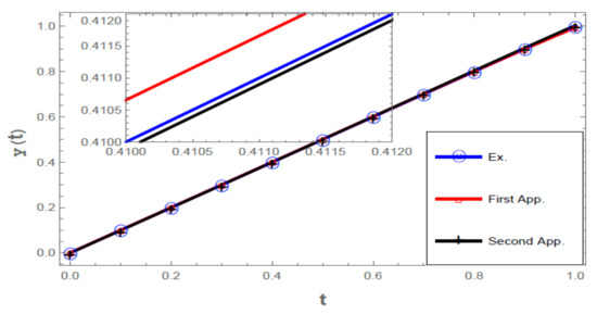
The exact solution of (27) and (28) is $y\left(t\right)=t$, we use Picard’s method to estimate the solution of (27) and (28).

$$\begin{array}{ccc}\hfill y_n\left(t\right)& =& \frac{1}{2}\left[\frac{1}{2}-{\int }_0^1{\int }_0^{\theta }\left(1-\frac{s^5}{16}+\left(\frac{1}{32}(s+s^5)\right)y_{n-1}\left({\int }_0^{s^2}\frac{y_{n-1}\left(u\right)}{{(1+y_{n-1}^2\left(u\right))}^2}\mathrm{d}u\right)\right)\mathrm{d}s\mathrm{d}\theta \right]\hfill \\ & & +{\int }_0^t\left(1-\frac{s^5}{16}{t}^2+\left(\frac{1}{32}(s+s^5)\right)y_{n-1}\left({\int }_0^{s^2}\frac{y_{n-1}\left(u\right)}{{(1+y_{n-1}^2\left(u\right))}^2}\mathrm{d}u\right)\right)\mathrm{d}s.\hfill \end{array}$$

(30)

$$y_0\left(t\right)=\frac{1}{4}$$

(31)

and

$$y\left(t\right)=\underset{n\to \infty }{lim}{y}_n\left(t\right).$$

Figure 1 shows the valuesobtained from the exact solution, the first and the second iterations for different values of t, the three lines in Figure 1 semi coincide; at the top of Figure 1, the lines have been enlarged to show the difference between them.

7. Conclusions

In this work, the existence of an absolutely continuous solution using Schauder’s fixed point theorem, the uniqueness solution and the continuous dependence of the functional differential inclusion with self-dependence on a nonlinear delay integral operator were studied. Some examples were introduced to illustrate the benefits of our results. Lastly, the Picard method was used to estimate the solution of a given example and plot the solution.

References

1. Hale, J.K. Theory of Functional Differential Equations; Springer: New York, NY, USA, 1977. [Google Scholar]
2. El-Sayed, A.M.A.; Ahmed, R.G. Infinite point and Riemann–Stieltjes integral conditions for an integro–differential equation. Nonlinear Anal. Model. Control 2019, 24, 733–754. [Google Scholar] [CrossRef]
3. El-Sayed, A.M.A.; Ahmed, R.G. Solvability of a coupled system of functional integro–differential equations with infinite point and Riemann–Stieltjes integral conditions. Appl. Math. Comput. 2020, 370, 124918. [Google Scholar] [CrossRef]
4. El-Sayed, A.M.A.; Ahmed, R.G. Existence of Solutions for a Functional Integro-Differential Equation with Infinite Point and Integral Conditions. Int. J. Appl. Comput. Math. 2019, 5, 108. [Google Scholar] [CrossRef]
5. El-Sayed, A.M.A.; Ahmed, R.G. Solvability of the functional integro-differential equation with self-reference and state-dependence. J. Nonlinear Sci. Appl. 2020, 13, 1–8. [Google Scholar] [CrossRef] [Green Version]
6. Srivastava, H.M.; El-Sayed, A.M.A.; Gaafar, F.M. A Class of Nonlinear Boundary Value Problems for an Arbitrary Fractional-Order Differential Equation with the Riemann-Stieltjes Functional Integral and Infinite-Point Boundary Conditions. Symmetry 2018, 10, 508. [Google Scholar] [CrossRef] [Green Version]
7. Zhong, Q.; Zhang, X. Positive solution for higher-order singular infinite-point fractional differential equation with p-Laplacian. Adv. Differ. Equ. 2016, 2016, 11. [Google Scholar] [CrossRef] [Green Version]
8. Zhang, X.; Liu, L.; Wu, Y.; Zou, Y. Fixed-point theorems for systems of operator equations and their applications to the fractional differential equations. J. Funct. Spaces 2018, 2018, 7469868. [Google Scholar] [CrossRef]
9. Ge, F.; Zhou, H.; Kou, C. Existence of solutions for a coupled fractional differential equations with infinitely many points boundary conditions at resonance on an unbounded domain. Differ. Equ. Dyn. Syst. 2019, 24, 395–411. [Google Scholar] [CrossRef]
10. El-Owaidy, H.; El-Sayed, A.M.A.; Ahmed, R.G. On an Integro–Differential equation of arbitary (fractional) orders with nonlocal integral and Infinite Point boundary Conditions. Fract. Differ. Calc. 2019, 9, 227–242. [Google Scholar] [CrossRef] [Green Version]
11. Bacotiu, C. Volterra-fredholm nonlinear systems with modified argument via weakly picard operators theory. Carpathian J. Math. 2008, 24, 1–9. [Google Scholar]
12. Benchohra, M.; Darwish, M.A. On unique solvability of quadratic integral equations with linear modification of the argument. Miskolc Math. Notes 2009, 10, 3–10. [Google Scholar] [CrossRef]
13. Buica, A. Existence and continuous dependence of solutions of some functional-differential equations. Semin. Fixed Point Theory A Publ. Semin. Fixed Point Theory-Cluj-Napoca 1995, 3, 1–14. [Google Scholar]
14. El-Sayed, A.M.A.; El-Owaidy, H.; Ahmed, R.G. Solvability of a boundary value problem of self–reference functional differential equation with infinite point and integral conditions. J. Math. Comput. Sci. 2020, 21, 296–308. [Google Scholar] [CrossRef]
15. Zhang, P.; Gong, X. Existence of solutions for iterative differential equations. Electron. J. Differ. Equ. 2014, 2014, 1–10. [Google Scholar]
16. Stanek, S. Globel properties of solutions of the functional differenatial equation x(t)x′(t)=kx(x(t)),0<|k|<1. Funct. Differ. Equ. 2002, 9, 527–550. [Google Scholar]
17. Berinde, V. Existence and approximation of solutions of some first order iterative differential equations. Miskolc Math. Notes 2010, 11, 13–26. [Google Scholar] [CrossRef]
18. Eder, E. The functional differential equation x′(t)=x(x(t)). J. Differ. Equ. 1984, 54, 390–400. [Google Scholar] [CrossRef] [Green Version]
19. Wang, K. On the equation x′(t)=f(x(x(t))). Funkcialaj Ekvacioj 1990, 33, 405–425. [Google Scholar]
20. Feckan, M. On a certain type of functional differential equations. Math. Slovaca 1993, 43, 39–43. [Google Scholar]
21. Stanek, S. Global properties of decreasing solutions of the equation x′(t)=x(x(t))+x(t). Funct. Differ. Equ. 1997, 4, 191–213. [Google Scholar]
22. Kolomogorov, A.N.; Fomin, S.V.; Kirk, W.A. Inroductory Real Analysis; Dover Publication Inc.: Mineola, NY, USA, 1975. [Google Scholar]
23. Goebel, K.; Kirk, W.A. Topics in Metric Fixed Point Theory; Cambirdge Universty Press: New York, NY, USA, 1990. [Google Scholar]
Figure 1. Exact solution, first approximation and second approximation.
Mathematics 10 02420 g001
Publisher’s Note: MDPI stays neutral with regard to jurisdictional claims in published maps and institutional affiliations.