Adaptive Neural Tracking Control for Nonstrict-Feedback Nonlinear Systems with Unknown Control Gains via Dynamic Surface Control Method

Abstract

This paper addresses the tracking control problem of nonstrict-feedback systems with unknown control gains. The dynamic surface control method, Nussbaum gain function control technique, and radial basis function neural network are applied for the design of virtual control laws, and adaptive control laws. Then, an adaptive neural tracking control law is proposed in the last step. By using the dynamic surface control method, the “explosion of complexity” problem of conventional backstepping is avoided. Based on the application of the Nussbaum gain function control technique, the unknown control gain problem is well solved. With the help of the radial basis function neural network, the unknown nonlinear dynamics are approximated. Furthermore, through Lyapunov stability analysis, it is proved that the proposed control law can guarantee that all signals in the closed-loop system are bounded and the tracking error can converge to an arbitrarily small domain of zero by adjusting the design parameters. Finally, two examples are provided to illustrate the effectiveness of the proposed control law.

1. Introduction

During the last few decades, control design and analysis for nonstrict-feedback nonlinear systems have been reported in much literature [1,2,3]. The adaptive control problems of nonstrict-feedback nonlinear systems with uncertain dynamics [4], state constraints [5], actuator faults [6], and time delay [7] have been solved by scholars. In addition, many control strategies, such as the finite-time adaptive output-feedback control law [8], the smooth-switching adaptive neural control law [9], the event-triggered-based adaptive neural network control law [10], and references therein, have been developed. To further deal with uncertain dynamics and unknown nonlinear functions, the fuzzy-logic system and neural networks are widely used as approximators of unknown dynamics [5,6,11,12]. For example, in [13], a fuzzy-logic system is applied to identify unknown nonlinear functions, and a fuzzy-based decentralized control scheme is proposed to ensure all signals are bounded. In [14], an adaptive neural-network command-filtered control law is presented, where the boundlessness of all variables is guaranteed by using the presented control law. As a powerful tool for dealing with uncertain systems, the backstepping control method and dynamic surface control technique are widely used to design the final control law.

The backstepping control method decomposes the n-order complex systems into several subsystems and designs virtual control laws for each step to realize the design of the final control law. In [15,16], the backstepping control method was applied to construct the adaptive neural network control law. In [17], an adaptive backstepping quantized control scheme was presented to ensure the stability of the given system. In [18], a command filter-based adaptive finite-time backstepping control law was designed that ensured that the position tracking error converged to the desired neighborhood in finite time. Nevertheless, when the backstepping control method is adopted, the repeated differential of virtual control will inevitably lead to computational complexity. To solve this problem, other control strategies have been considered by researchers. For instance, the backstepping sliding mode control method was designed in [19,20] and the command filtered backstepping control method studied in [21,22].

Although the above methods can effectively solve the control problems of complex systems, the dynamic surface control method is also widely used. In the dynamic surface control method, the first-order filter is introduced to construct the filtering error signal so as to realize the design of the final control law. In [23,24], adaptive fuzzy dynamic surface control laws were designed to ensure that the tracking error converged to a small neighborhood of zero. In [25,26], adaptive neural network dynamic surface control laws were proposed in which the problems of global asymptotic stability and prespecified tracking accuracy respectively, are achieved.

In some physical systems, the control gain signs may not always be known, due to the influence of external factors. If there is no prior knowledge about the control gain, the control law design will become much more difficult. Fortunately, the Nussbaum gain function technique has been used by many researchers to solve this problem. This method was proposed by Nussbaum [27], and can effectively solve the control problem of a system with unknown control gain. In [28,29,30], adaptive control laws were addressed by applying the Nussbaum gain function method for nonlinear systems with unknown control directions. In [31], the authors proposed an observer-based adaptive fuzzy output-feedback control law for uncertain nonlinear systems with input quantization and unknown control direction in which the control law design combines the backstepping technique and Nussbaum function. Furthermore, the consensus control problems of multiagent systems with unknown control directions were studied in [32,33], where the improved Nussbaum-type gain functions were used to design the consensus control laws. However, it is worth noting that the unknown control gains of the nonstrict-feedback systems may exist in each subsystem.

Inspired by the above results, this paper addresses an adaptive dynamic surface control law for the tracking control problem of the nonstrict-feedback nonlinear systems with unknown control gains. The radial basis function neural network (RBFNN) and Nussbaum gain function control technique are introduced to design the final control law. The main contributions of this paper are as follows: (1) a class of nonstrict-feedback nonlinear systems with unknown control gains is considered, and differently from [25,26], the unknown control gain exists in each subsystem; (2) compared with [28,29], in this paper, the Nussbaum gain function is considered in each step of recursive design, and thus the design of the virtual control law can be realized by using the dynamic surface control technique; and (3) the proposed control law can guarantee that all signals in the closed-loop system are bounded and the tracking error can converge to an arbitrarily small domain of zero.

The main arrangement of this paper is as follows. The problem formulation and preliminaries are given in Section 2. Section 3 displays the process of control law design and stability analysis. Numeric simulations and conclusions are provided in Section 4 and Section 5, respectively.

2. Problem Formulation and Preliminaries

A class of nonstrict-feedback nonlinear systems with unknown control gains is described as

$$\begin{array}{l}{\dot{x}}_i={\theta }_i{x}_{i+1}+f_i({\overline{x}}_i),i=1,\dots ,n-1\\ {\dot{x}}_n={\theta }_{n}u+f_n({\overline{x}}_n)\\ y=x_1\end{array}$$

(1)

where ${\overline{x}}_i={\left[x_1,\cdots ,x_i\right]}^T$, $i=1,\cdots ,n$, represent state vectors; $u\in R$ and $y\in R$ are control input and system output, respectively; ${\theta }_i$, $i=1,\cdots ,n$, represent the unknown control gains; and $f_i({\overline{x}}_i)$ and $f_n({\overline{x}}_n)$ are continuous unknown nonlinear functions. For convenience, the functions $f_i({\overline{x}}_i)$ and $f_n({\overline{x}}_n)$ are denoted by $f_i$ and $f_n$, respectively.

The control goal of this paper is to design the control law $u(t)$ for the system (1) so that the system’s output $y$ can track the reference signal $y_d$, despite the presence of unknown control gains.

Assumption 1.

The sign of control gains${\theta }_i$, $i=1,\cdots ,n$is assumed to be strictly positive or negative. Without loss of generality, it is assumed to be positive in this paper. Furthermore, there exists the unknown positive constant${\theta }_M$such that${\theta }_i\le {\theta }_M$.

Assumption 2.

The reference signal$y_d$is sufficiently smooth, that is, there exists a positive constant$G_0$such that${\Omega }_0:=\left\{(y_d,{\dot{y}}_d,{\ddot{y}}_d):y_d^2+{\dot{y}}_d^2+{\ddot{y}}_d^2\le G_0\right\}$.

Note 1. Assumptions 1 and 2 are normal assumptions that are found in much literature [5,10,23,26]. The application of these assumptions does not impose strong restrictions on the nonstrict-feedback system.

To facilitate the control system design, the following definition and lemmas are provided.

 Definition 1 

([30]). For a smooth function $\mathcal{N}(\kappa )$ , if the following properties are held

$$\{\begin{array}{l}\underset{s\to \infty }{\lim }\sup \frac{1}{s}{\displaystyle {\int }_0^s\mathcal{N}(\kappa )d}\kappa =+\infty \\ \underset{s\to \infty }{\lim }\inf \frac{1}{s}{\displaystyle {\int }_0^s\mathcal{N}(\kappa )d}\kappa =-\infty \end{array}$$

(2)

then $\mathcal{N}(\kappa )$ is called a Nussbaum gain function. In this paper, the Nussbaum gain function is considered as $\mathcal{N}(\kappa )={\kappa }^2\cos (\kappa )$.

 Lemma 1 

([30]). Let $V(t)\ge 0$ and $\kappa (t)$ be smooth functions defined on $[0,t_f)$, and $\mathcal{N}(\kappa )$ be the Nussbaum gain function. If the following inequality holds

$$V(t)\le e^{-k_{0}t}{\displaystyle {\int }_0^t{e}^{k_0\tau }\left(\varpi \mathcal{N}(\kappa (\tau ))+1\right)}\dot{\kappa }(\tau )d\tau +c_0,t\in [0,t_f)$$

(3)

then $V(t)$, $\kappa (t)$ and ${\displaystyle {\int }_0^t{e}^{k_0\tau }\left(\varpi \mathcal{N}(\kappa (\tau ))+1\right)}\dot{\kappa }(\tau )d\tau$ are bounded on $[0,t_f)$, where $\varpi$ , $c_0$ and $k_0$ are positive constants.

 Lemma 2 

([7]). For any continuous function $h(\mathit{x})$ over a compact set $\Omega \subset R^n$, there exists an RBFNN ${({\mathit{W}}^{*})}^T\phi {(\mathit{x})}^{*}$ such that

$$h(\mathit{x})={({\mathit{W}}^{*})}^T\mathbf{\phi }(\mathit{x})+\epsilon (\mathit{x}),\forall \mathit{x}\in \Omega$$

(4)

where ${\mathit{W}}^{*}\in R^l$ is the optimal weight vector, $l>1$ is the neural network node number,$\epsilon (\mathit{x})$ is the approximation error and satisfies $\left|\epsilon (\mathit{x})\right|\le {\epsilon }^{*}$, and $\mathbf{\phi }(\mathit{x})={\left[{\phi }_1(\mathit{x}),\cdots ,{\phi }_l(\mathit{x})\right]}^T\in R^l$ is the Gaussian-like basis function vector with

$${\phi }_i(\mathit{x})=\exp \left(-\frac{{(\mathit{x}-{\varsigma }_i)}^T(\mathit{x}-{\varsigma }_i)}{{\sigma }^2}\right),i=1,2,\cdots ,l$$

(5)

with ${\varsigma }_i={\left[{\varsigma }_{i1},\cdots ,{\varsigma }_{in}\right]}^T$ the center of the basis function, and $\sigma$ is the width of the Gaussian function.

 Lemma 3 

([23]). For any $b\in R$ and $\vartheta >0$, the inequality $0\le \left|b\right|-b\tanh (b/\vartheta )\le 0.2785\vartheta$ holds.

 Lemma 4 

([25]). For any $x\in R$ and $y\in R$, the following inequality holds

$$xy\le \frac{{\nu }^p}{p}{\left|x\right|}^p+\frac{1}{q{\nu }^q}{\left|y\right|}^q$$

(6)

where $\nu >0$, $p>1$, $q>1$ and $(p-1)(q-1)=1$.

3. Control Law Design and Stability Analysis

In this section, the control design procedure for the system (1) is developed, which is mainly based on the dynamic surface control method and neural network approximator.

3.1. Adaptive Neural Tracking Control Law Design

According to the system (1), the coordinate transformation error is defined as

$$z_i=x_i-y_{i,d},i=1,2,\cdots ,n$$

(7)

where $y_{1,d}=y_d$, $y_{i,d}$ for $i=2,\cdots ,n$ are the output of first-order filter with the virtual control law ${\alpha }_{i-1}$ as the input, which is given as

$$\begin{array}{l}{\tau }_i{\dot{y}}_{i,d}+y_{i,d}={\alpha }_{i-1},i=2,\cdots ,n\\ y_{i,d}(0)={\alpha }_{i-1}(0)\end{array}$$

(8)

where ${\tau }_i$ is a positive constant to be designed.

Furthermore, the filter error signal is constructed as

$$s_i=y_{i,d}-{\alpha }_{i-1},i=2,\cdots ,n$$

(9)

In the following analysis, the actual control law will be presented through recursive design.

Step i  ($i=1,2,\cdots ,n-1$). Taking the time derivative of $z_i$ in (7) obtains

$$\begin{array}{l}{\dot{z}}_i={\theta }_i{x}_{i+1}+f_i-{\dot{y}}_{i,d}\\ ={\theta }_i{\alpha }_i+{\theta }_i{z}_{i+1}+{\theta }_i{s}_{i+1}+f_i-{\dot{y}}_{i,d}\end{array}$$

(10)

Let ${\overline{V}}_i=z_i^2/2$, then the time derivative of ${\overline{V}}_i$ is

$${\dot{\overline{V}}}_i=z_i\left({\theta }_i{\alpha }_i+{\theta }_i{z}_{i+1}+{\theta }_i{s}_{i+1}+f_i-{\dot{y}}_{i,d}\right)$$

(11)

Using Lemma 4, we have

$${\theta }_i{z}_i{z}_{i+1}\le \frac{{\theta }_i^2{z}_i^2}{2}+\frac{z_{i+1}^2}{2}$$

(12)

$${\theta }_i{z}_i{s}_{i+1}\le \frac{{\theta }_i^2{z}_i^2}{2}+\frac{s_{i+1}^2}{2}$$

(13)

Substituting (12) and (13) into (11), one gets

$${\dot{\overline{V}}}_1\le {\theta }_i{z}_i{\alpha }_i+\frac{1}{2}{z}_{i+1}^2+\frac{1}{2}{s}_{i+1}^2+z_i{F}_i-z_i{\dot{y}}_{i,d}$$

(14)

where $F_i={\theta }_i^2{z}_i+f_i$.

$F_i$ contains unknown function $f_i$ and unknown gain ${\theta }_i$, such that it cannot be directly used to control law design. According to Lemma 2, an RBFNN ${({\mathit{W}}_i^{*})}^T{\mathbf{\phi }}_i({\mathit{X}}_i)$ with input ${\mathit{X}}_i={\left[y_{1,d},\cdots ,y_{i,d},x_1,\cdots ,x_i\right]}^T$ is considered to approximate $F_i$, such that

$$F_i={({\mathit{W}}_i^{*})}^T{\mathbf{\phi }}_i({\mathit{X}}_i)+{\epsilon }_i({\mathit{X}}_i),\left|{\epsilon }_i({\mathit{X}}_i)\right|\le {\epsilon }_i^{*}$$

(15)

where ${\epsilon }_i({\mathit{X}}_i)$ is the approximation error and ${\epsilon }_i^{*}$ is a positive constant.

To stabilize the subsystem, the virtual control law ${\alpha }_i$ and adaptive control laws are designed as

$${\alpha }_i={\mathcal{N}}_i({\kappa }_i){\beta }_i$$

(16)

$${\beta }_i={({\widehat{\mathit{W}}}_i)}^T{\mathbf{\phi }}_i+{\epsilon }_i^{*}\tanh (\frac{{\epsilon }_i^{*}{z}_i}{\vartheta })+{\lambda }_i{z}_i-{\dot{y}}_{i,d}$$

(17)

$${\dot{\kappa }}_i=z_i\left({({\widehat{\mathit{W}}}_i)}^T{\mathbf{\phi }}_i+{\epsilon }_i^{*}\tanh (\frac{{\epsilon }_i^{*}{z}_i}{\vartheta })+{\lambda }_i{z}_i-{\dot{y}}_{i,d}\right)$$

(18)

$${\dot{\widehat{\mathit{W}}}}_i={\eta }_i\left(z_i{\mathbf{\phi }}_i-{\gamma }_i{\widehat{\mathit{W}}}_i\right)$$

(19)

where ${\widehat{\mathit{W}}}_i$ is the estimate of ${\mathit{W}}_i^{*}$ and $\vartheta$, ${\lambda }_i$, ${\eta }_i$ and ${\gamma }_i$ are positive constants to be designed.

Define the Lyapunov function candidate as

$$V_i={\overline{V}}_i+\frac{1}{2{\eta }_i}{({\tilde{\mathit{W}}}_i)}^T{\tilde{\mathit{W}}}_i$$

(20)

where ${\tilde{\mathit{W}}}_i={\mathit{W}}_i^{*}-{\widehat{\mathit{W}}}_i$, and ${\dot{\tilde{\mathit{W}}}}_i=-{\dot{\widehat{\mathit{W}}}}_i$.

The time derivative of (20) is

$${\dot{V}}_i={\dot{\overline{V}}}_i-\frac{1}{{\eta }_i}{({\tilde{\mathit{W}}}_i)}^T{\dot{\widehat{\mathit{W}}}}_i$$

(21)

Substituting (14)–(19) into (21) and considering Lemma 3, one has

$${\dot{V}}_i\le \left({\theta }_i{\mathcal{N}}_i({\kappa }_i)+1\right){\dot{\kappa }}_i-{\lambda }_i{z}_i^2+\frac{1}{2}{z}_{i+1}^2+\frac{1}{2}{s}_{i+1}^2+{\gamma }_i{({\tilde{\mathit{W}}}_i)}^T{\widehat{\mathit{W}}}_i+0.2785\vartheta$$

(22)

Step$n$. This is the last step, and the actual control law will be presented in this step. Taking the time derivative of $z_n$ in (7) yields

$${\dot{z}}_n={\theta }_{n}u+f_n-{\dot{y}}_{n,d}$$

(23)

An RBF neural network ${({\mathit{W}}_n^{*})}^T{\mathbf{\phi }}_n({\mathit{X}}_n)$ with input ${\mathit{X}}_n={\left[x_1,\cdots ,x_n\right]}^T$ is considered to approximate $f_n$, such that

$$f_n={({\mathit{W}}_n^{*})}^T{\mathbf{\phi }}_n({\mathit{X}}_n)+{\epsilon }_n({\mathit{X}}_n),\left|{\epsilon }_n({\mathit{X}}_n)\right|\le {\epsilon }_n^{*}$$

(24)

where ${\epsilon }_n({\mathit{X}}_n)$ is the approximation error and ${\epsilon }_n^{*}$ is a positive constant.

Let ${\overline{V}}_n=z_n^2/2$ and noting (24), then the time derivative of ${\overline{V}}_n$ is

$${\dot{\overline{V}}}_n={\theta }_n{z}_{n}u+z_n{({\mathit{W}}_n^{*})}^T{\mathbf{\phi }}_n+z_n{\epsilon }_n-z_n{\dot{y}}_{n,d}$$

(25)

Now, we design the actual control law $u(t)$ and adaptive control laws as

$$u(t)={\mathcal{N}}_n({\kappa }_n){\beta }_n$$

(26)

$${\beta }_n={({\widehat{\mathit{W}}}_n)}^T{\mathbf{\phi }}_n+{\epsilon }_n^{*}\tanh (\frac{{\epsilon }_n^{*}{z}_n}{\vartheta })+{\lambda }_n{z}_n-{\dot{y}}_{n,d}$$

(27)

$${\dot{\kappa }}_n=z_n\left({({\widehat{\mathit{W}}}_n)}^T{\mathbf{\phi }}_n+{\epsilon }_n^{*}\tanh (\frac{{\epsilon }_n^{*}{z}_n}{\vartheta })+{\lambda }_n{z}_n-{\dot{y}}_{n,d}\right)$$

(28)

$${\dot{\widehat{\mathit{W}}}}_n={\eta }_n\left(z_n{\mathbf{\phi }}_n-{\gamma }_n{\widehat{\mathit{W}}}_n\right)$$

(29)

where ${\widehat{\mathit{W}}}_n$ is the estimate of ${\mathit{W}}_n^{*}$ and $\vartheta$, ${\lambda }_n$, ${\eta }_n$ and ${\gamma }_n$ are positive constants to be designed.

Define the Lyapunov function candidate as

$$V_n={\overline{V}}_n+\frac{1}{2{\eta }_n}{({\tilde{\mathit{W}}}_n)}^T{\tilde{\mathit{W}}}_n$$

(30)

where ${\tilde{\mathit{W}}}_n={\mathit{W}}_n^{*}-{\widehat{\mathit{W}}}_n$, and ${\dot{\tilde{\mathit{W}}}}_n=-{\dot{\widehat{\mathit{W}}}}_n$.

Along with (24)–(29), the time derivative of $V_n$ can be concluded as

$${\dot{V}}_n\le \left({\theta }_n{\mathcal{N}}_n({\kappa }_n)+1\right){\dot{\kappa }}_n-{\lambda }_n{z}_n^2+{\gamma }_n{({\tilde{\mathit{W}}}_n)}^T{\widehat{\mathit{W}}}_n+0.2785\vartheta$$

(31)

So far, the design process of the adaptive neural tracking control law is completed.

3.2. Stability Analysis

Theorem 1.

Consider the nonstrict-feedback nonlinear system (1) with unknown control gains under Assumptions 1 and 2, the virtual control laws are designed as (16) with the adaptive control laws given by (18) and (19), and the actual control law is designed as (26) with the adaptive control laws given by (28) and (29), and there exist${\lambda }_i$,${\eta }_i$and${\gamma }_i$for$i=1,\cdots ,n$,${\tau }_i$for$i=2,\cdots ,n$, and$\vartheta$, such that all signals in the closed-loop system are bounded and the tracking error can converge to an arbitrarily small domain of zero, that is,${\lim }_{t\to \infty }\left|z_1\right|\le \sqrt{2a_1/\rho }$.

Proof. 

Considering (8) and (9), we have ${\dot{y}}_{i,d}=-s_i/{\tau }_i$, and the time derivative of $s_i$ yielding

$$\begin{array}{l}{\dot{s}}_i=-\frac{s_i}{{\tau }_i}-{\dot{\alpha }}_{i-1}\\ =-\frac{s_i}{{\tau }_i}-\left(\frac{\partial {\alpha }_{i-1}}{\partial {\kappa }_{i-1}}{\dot{\kappa }}_{i-1}+\frac{\partial {\alpha }_{i-1}}{\partial {\widehat{\mathit{W}}}_{i-1}}{\dot{\widehat{\mathit{W}}}}_{i-1}+\frac{\partial {\alpha }_{i-1}}{\partial z_{i-1}}{\dot{z}}_{i-1}+\frac{\partial {\alpha }_{i-1}}{\partial {\dot{y}}_{i-1,d}}{\ddot{y}}_{i-1,d}\right)\\ =-\frac{s_i}{{\tau }_i}+G_i\left(z_1,\cdots ,z_i,s_2,\cdots ,s_i,{\widehat{\mathit{W}}}_1,\cdots ,{\widehat{\mathit{W}}}_{i-1},y_d,{\dot{y}}_d,{\ddot{y}}_d\right)\end{array}$$

(32)

where $i=2,\cdots ,n$, $G_i(\cdot )$ is the introduced non-negative continuous function.

Let the compact set ${\Omega }_1$ as

$${\Omega }_1:=\left\{(z_1,\cdots ,z_i,s_2,\cdots ,s_i,{\widehat{\mathit{W}}}_1,\cdots ,{\widehat{\mathit{W}}}_i,y_d,{\dot{y}}_d,{\ddot{y}}_d):{\displaystyle \sum _{i=1}^n{z}_i^2}+{\displaystyle \sum _{i=1}^n\frac{1}{{\eta }_i}{({\tilde{\mathit{W}}}_i)}^T{\tilde{\mathit{W}}}_i}+{\displaystyle \sum _{i=2}^n{s}_i^2}\le 2q,i=1,\cdots ,n\right\}$$

and noting Assumption 2, we get ${\Omega }_0\times {\Omega }_1$ is also a compact set. Therefore, there exists a positive constant $G_{i,M}$ in the compact set ${\Omega }_0\times {\Omega }_1$ such that $\left|G_i(\cdot )\right|\le G_{i,M}$ for $i=2,\cdots ,n$.

Furthermore, according to (7), (9), (19) and (32), we have

$$\left|{\dot{s}}_i+\frac{s_i}{{\tau }_i}\right|\le G_i\left(z_1,\cdots ,z_i,s_2,\cdots ,s_i,{\widehat{\mathit{W}}}_1,\cdots ,{\widehat{\mathit{W}}}_{i-1},y_d,{\dot{y}}_d,{\ddot{y}}_d\right)$$

(33)

and then,

$$s_i{\dot{s}}_i\le \left|s_i{G}_i(\cdot )\right|-\frac{s_i^2}{{\tau }_i}$$

(34)

Taking the Lyapunov function candidate as

$$V={\displaystyle \sum _{i=1}^n{V}_i}+\frac{1}{2}{\displaystyle \sum _{i=2}^n{s}_i^2}$$

(35)

It follows from (22), (31), and (34), the time derivative of (35) is

$$\begin{array}{l}\dot{V}\le -{\displaystyle \sum _{i=1}^n{\lambda }_i{z}_i^2}+\frac{1}{2}{\displaystyle \sum _{i=2}^n{z}_i^2}+\frac{1}{2}{\displaystyle \sum _{i=2}^n{s}_i^2}+{\displaystyle \sum _{i=1}^n{\gamma }_i{({\tilde{\mathit{W}}}_i)}^T{\widehat{\mathit{W}}}_i}+{\displaystyle \sum _{i=1}^n\left({\theta }_i{\mathcal{N}}_i({\kappa }_i)+1\right){\dot{\kappa }}_i}\\ +{\displaystyle \sum _{i=2}^n\left(\left|s_i{G}_i(\cdot )\right|-\frac{s_i^2}{{\tau }_i}\right)}+0.2785\vartheta n\end{array}$$

(36)

Considering Lemma 4, we get

$${({\tilde{\mathit{W}}}_i)}^T{\widehat{\mathit{W}}}_i={({\tilde{\mathit{W}}}_i)}^T({\mathit{W}}_i^{*}-{\tilde{\mathit{W}}}_i)\le -\frac{1}{2}{({\tilde{\mathit{W}}}_i)}^T{\tilde{\mathit{W}}}_i+\frac{1}{2}{({\mathit{W}}_i^{*})}^T{\mathit{W}}_i^{*}$$

(37)

$$\left|s_i{G}_i(\cdot )\right|\le \frac{s_i^2{G}_i^2(\cdot )}{2\sigma }+\frac{\sigma }{2}$$

(38)

where $\sigma$ is a positive constant.

Substituting (37) and (38) into (36) yields

$$\begin{array}{l}\dot{V}\le -{\lambda }_1{z}_1^2-{\displaystyle \sum _{i=2}^n\left({\lambda }_i-\frac{1}{2}\right)z_i^2}-{\displaystyle \sum _{i=1}^n({\eta }_i{\gamma }_i)\frac{1}{2{\eta }_i}{({\tilde{\mathit{W}}}_i)}^T{\tilde{\mathit{W}}}_i}-\frac{1}{2}{\displaystyle \sum _{i=2}^n\left(\frac{2}{{\tau }_i}-\frac{G_i^2(\cdot )}{\sigma }-1\right)s_i^2}\\ +{\displaystyle \sum _{i=1}^n\left({\theta }_i{\mathcal{N}}_i({\kappa }_i)+1\right){\dot{\kappa }}_i}+a_1\end{array}$$

(39)

where $a_1=0.2785\vartheta n+\sigma (n-1)/2+{\displaystyle {\sum }_{i=1}^n{\gamma }_i{({\mathit{W}}_i^{*})}^T{\mathit{W}}_i^{*}/2}$.

Taking

$$\begin{gathered} {\lambda }_1\ge \frac{\rho }{2} \\ {\lambda }_i\ge \frac{\rho +1}{2},i=2,\cdots ,n \\ {\eta }_i{\gamma }_i\ge \rho ,i=1,\cdots ,n \\ \frac{1}{{\tau }_i}\ge \frac{1}{2}+\frac{G_{i,M}^2}{2\sigma }+\frac{\rho }{2},i=2,\cdots ,n \end{gathered}$$

where $\rho$ is a positive constant to be designed. Then, we can rewrite (39) as

$$\dot{V}\le -\rho V+a_1+{\displaystyle \sum _{i=2}^n\left(\frac{G_i^2(\cdot )}{G_{i,M}^2}-1\right)\frac{s_i^2{G}_{i,M}^2}{\sigma }}+{\displaystyle \sum _{i=1}^n\left({\theta }_i{\mathcal{N}}_i({\kappa }_i)+1\right){\dot{\kappa }}_i}$$

(40)

It is obvious from (40) that $G_i^2(\cdot )/G_{i,M}^2-1\le 0$. Then, multiply by $e^{-\rho t}$ on both sides of (40), and integrate on $[0,t)$, we have

$$V\le e^{-\rho t}{\displaystyle \sum _{i=1}^n{\displaystyle {\int }_0^t{e}^{-\rho \tau }\left({\theta }_i{\mathcal{N}}_i({\kappa }_i)+1\right){\dot{\kappa }}_{i}d\tau }}+\left(V(0)-\frac{a_1}{\rho }\right)e^{-\rho t}+\frac{a_1}{\rho }$$

(41)

and further obtain that

$$V\le e^{-\rho t}{\displaystyle \sum _{i=1}^n{\displaystyle {\int }_0^t{e}^{-\rho \tau }\left({\theta }_i{\mathcal{N}}_i({\kappa }_i)+1\right)\dot{\kappa }d\tau }}+a_2$$

(42)

where $a_2=V(0)+a_1/\rho$.

Applying Lemma 1, we can get from (42) that ${\displaystyle {\sum }_{i=1}^n{\displaystyle {\int }_0^t{e}^{-\rho \tau }\left({\theta }_i{\mathcal{N}}_i({\kappa }_i)+1\right){\dot{\kappa }}_{i}d\tau }}$ are bounded. Without loss of generality, we assume that $\max {\displaystyle {\sum }_{i=1}^n{\displaystyle {\int }_0^t{e}^{-\rho \tau }\left({\theta }_i{\mathcal{N}}_i({\kappa }_i)+1\right){\dot{\kappa }}_{i}d\tau }}=A_0$. From (41), hence, one has

$$V\le \left(V(0)+A_0-\frac{a_1}{\rho }\right)e^{-\rho t}+\frac{a_1}{\rho }$$

(43)

Noting ${\overline{V}}_i=z_i^2/2$, (20) and (35), we have ${\displaystyle {\sum }_{i=1}^n{z}_i^2/2}\le V$. Considering (43), we can obtain that

$$\underset{t\to \infty }{\lim }\left|z_1\right|\le \sqrt{\frac{2a_1}{\rho }}$$

(44)

Note that $a_1/\rho$ depends on the design parameters ${\gamma }_i$, ${\lambda }_i$, ${\tau }_i$, and ${\eta }_i$. Therefore, we can adjust the design parameters so that the tracking error $z_1$ can converge to an arbitrarily small domain of zero. This completes the proof. □

Note 2. Theorem 1 displays that the designed adaptive laws and control law can ensure the convergence of tracking error. That is to say, the value of $a_1/\rho$ can be freely adjusted by selecting appropriate design parameters, namely, the tracking error $z_1$ can be arbitrarily small.

Note 3. It is observed (44) that the tracking error ${\lim }_{t\to \infty }\left|z_1\right|\le \sqrt{2a_1/\rho }$ can be designed as an arbitrarily small domain of zero by increasing $\rho$ or decreasing $a_1$. To increase the value of $\rho$, we can increase the value of parameters ${\lambda }_i$ and ${\eta }_i$, or decrease the value of the parameter ${\tau }_i$, and to decrease the value of $a_1$, we can decrease the value of parameter ${\gamma }_i$. However, the adjustment of these parameters may lead to larger amplitude of the control signal. Therefore, when selecting design parameters, appropriate trade-offs should be made between tracking control performance and control signal amplitude.

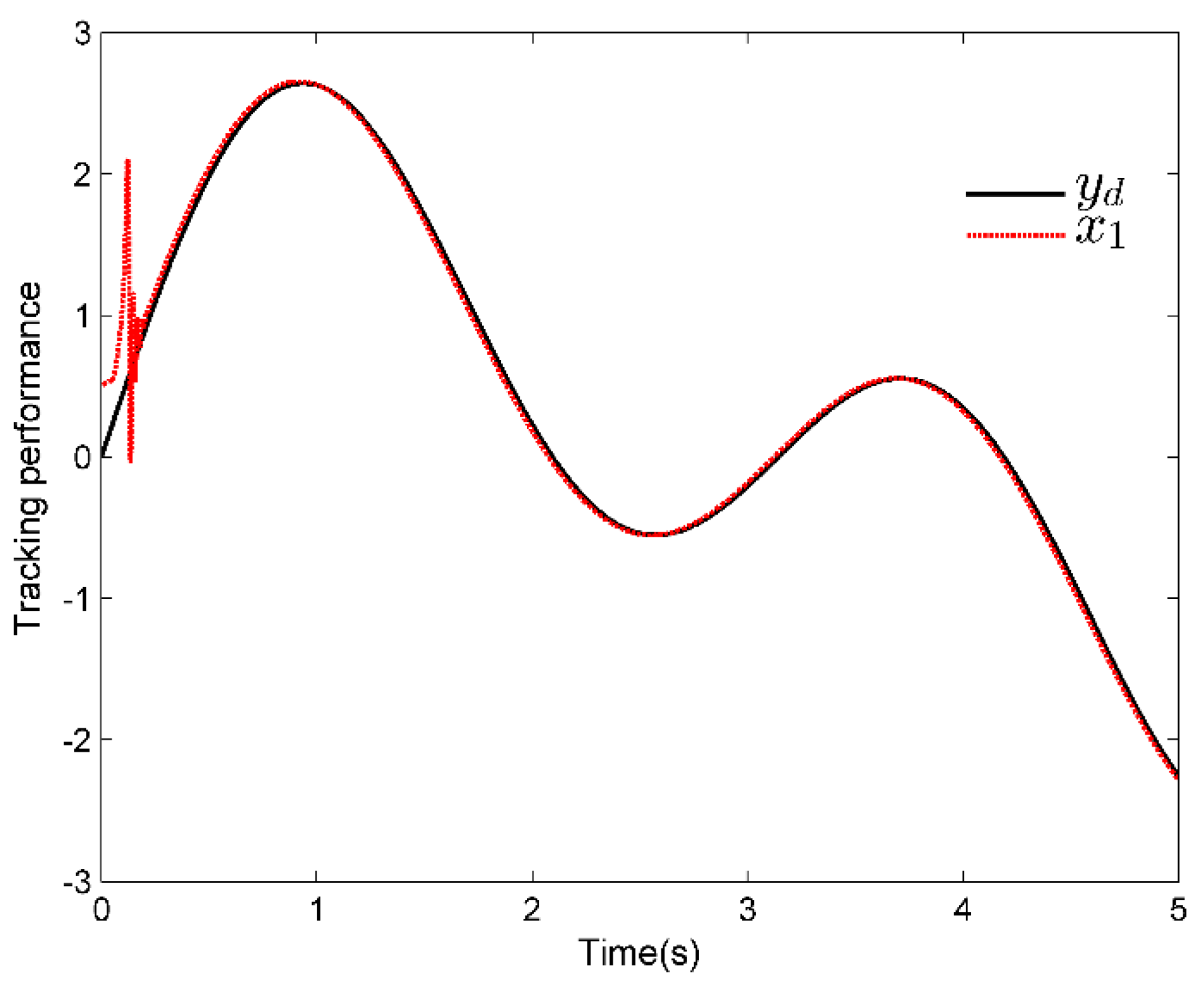
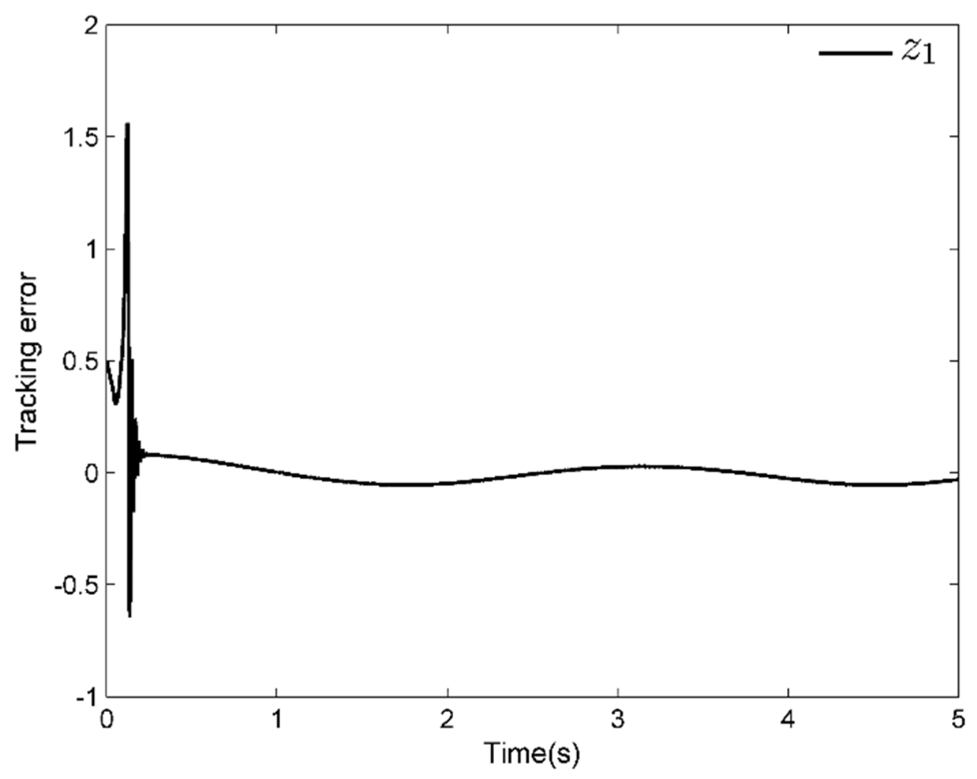
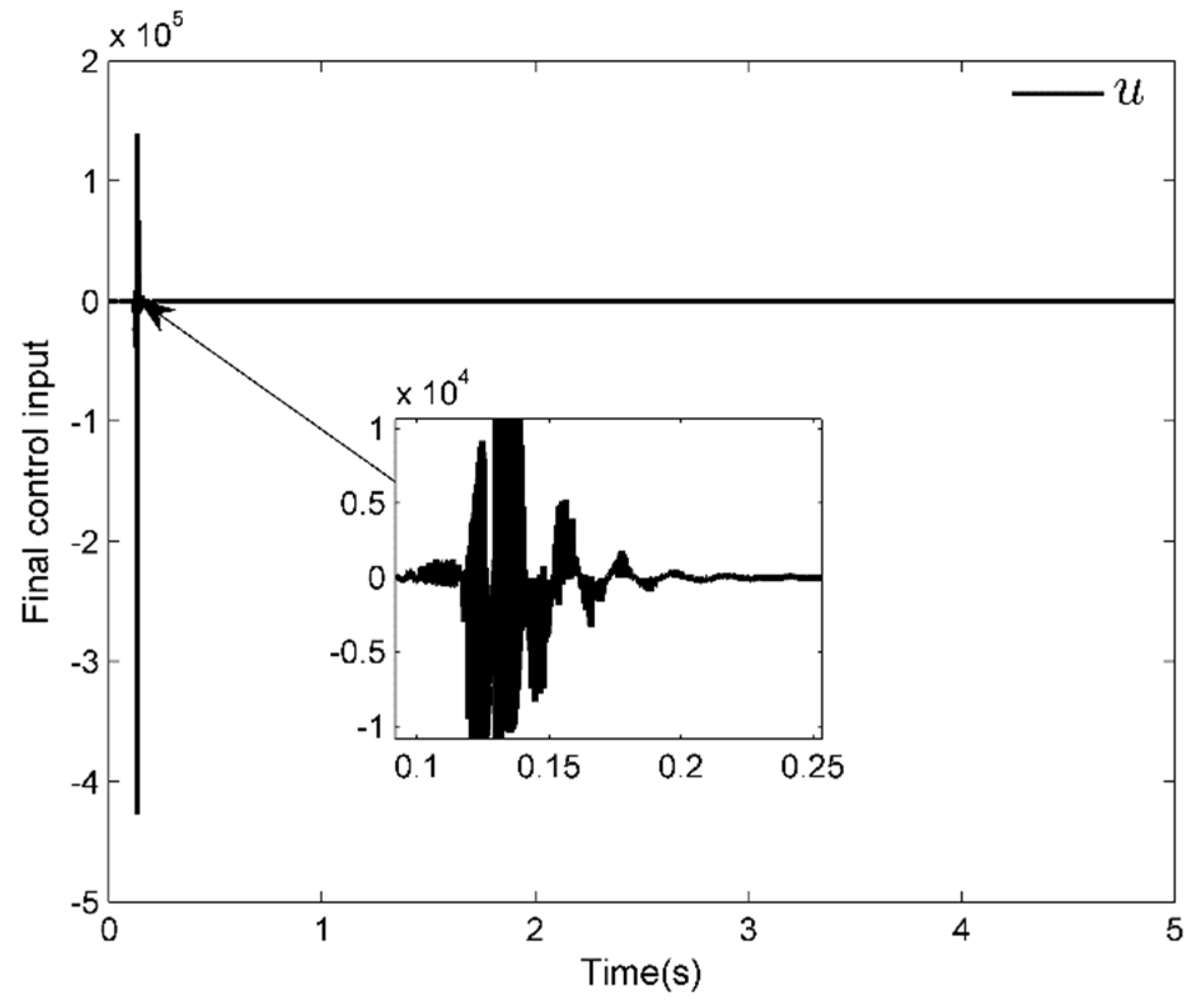
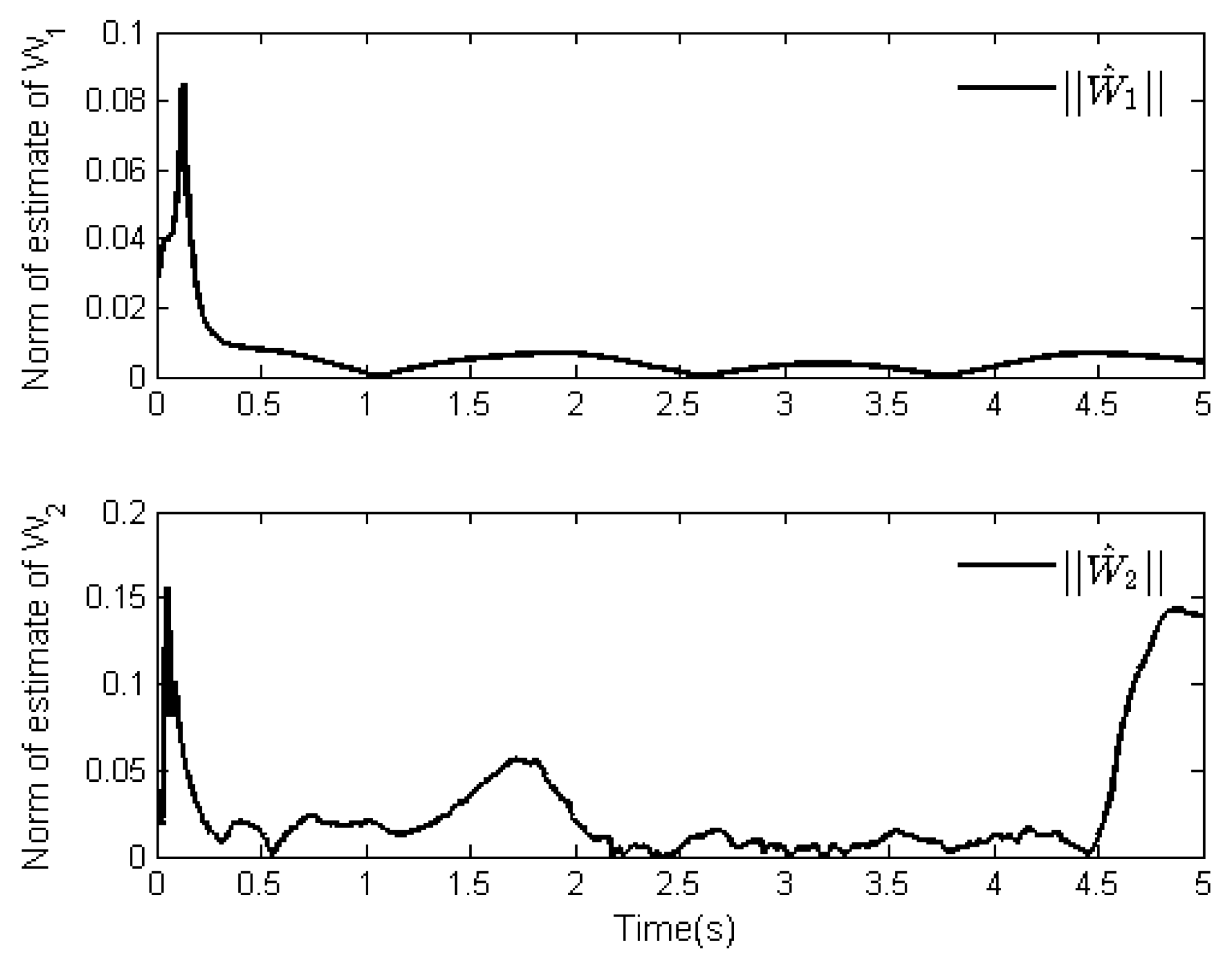
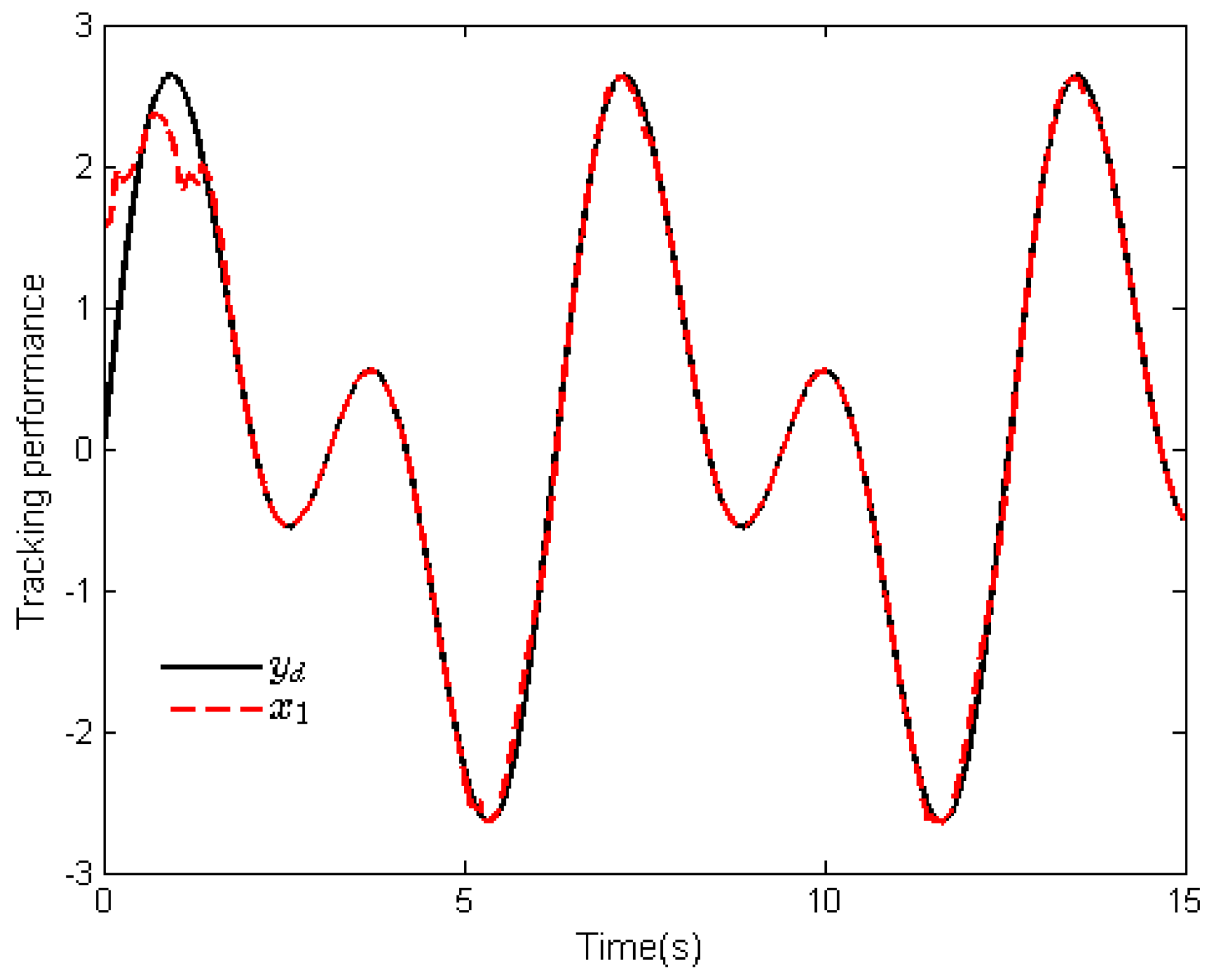
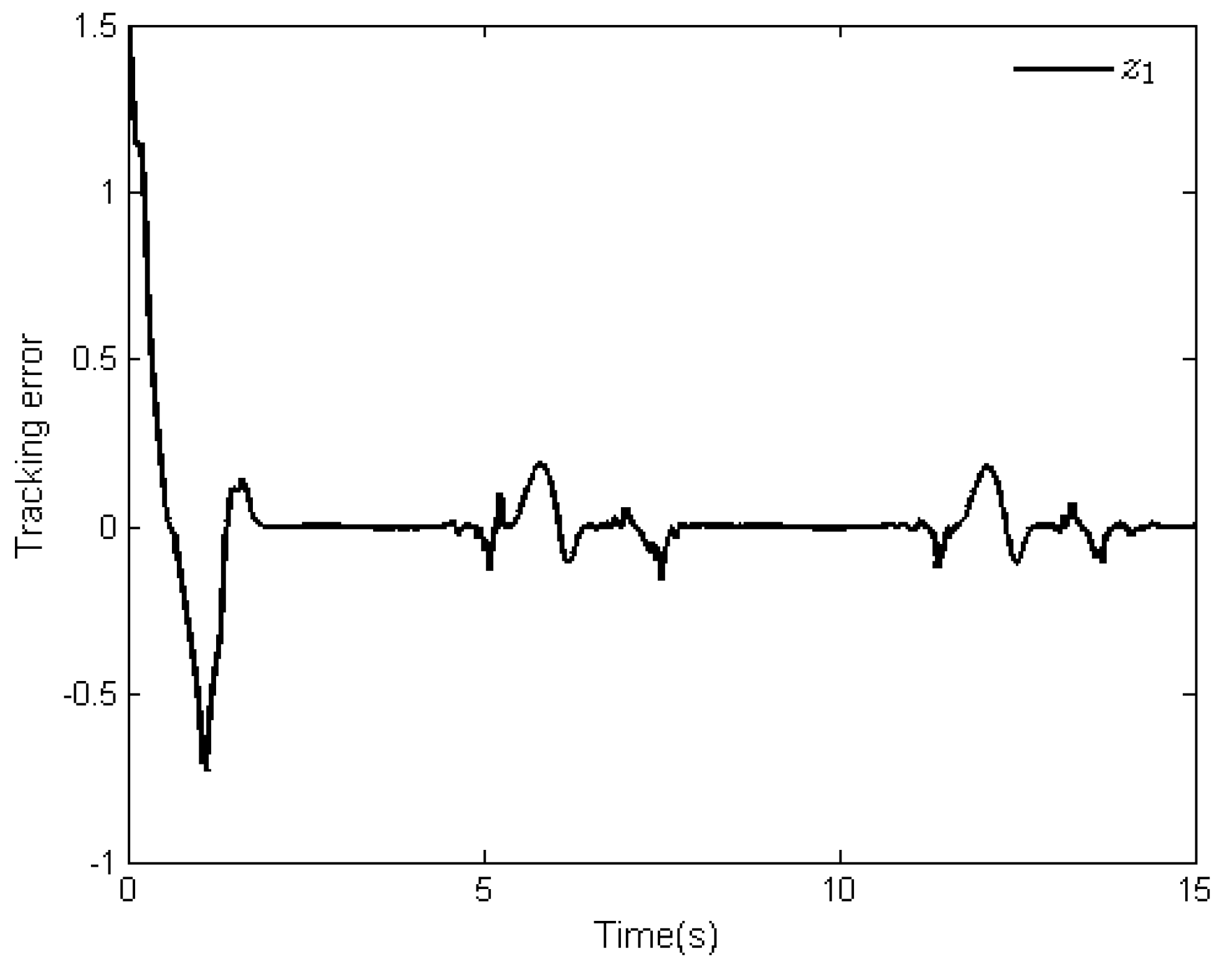
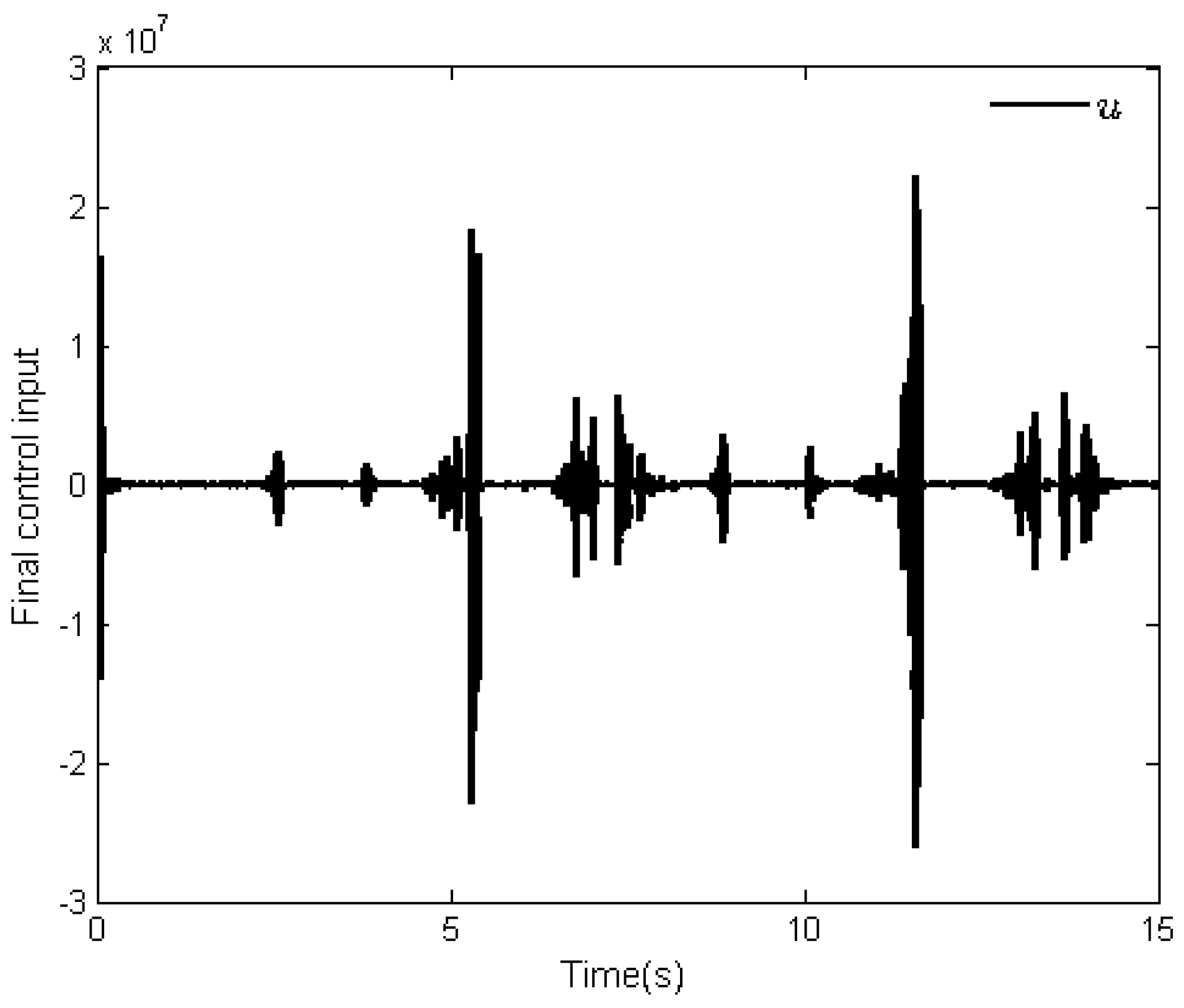
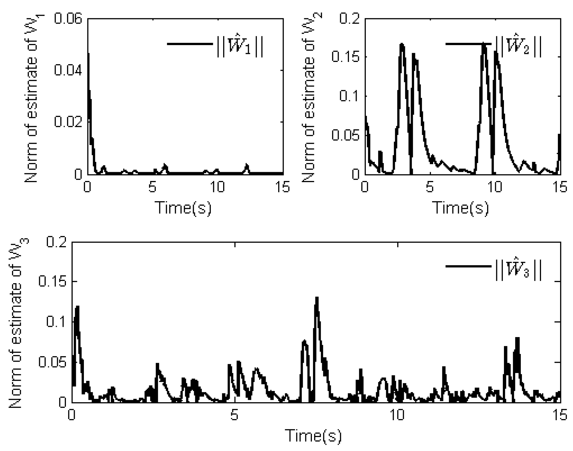
4. Simulation Analysis

In this section, two simulation examples are provided to illustrate the effectiveness of the proposed adaptive neural dynamic surface control law.

Example 1. Consider a class of nonstrict-feedback nonlinear systems as

$$\begin{array}{l}{\dot{x}}_1=3x_2+2x_1\sin (x_1)+x_1^2\\ {\dot{x}}_2=5u+\cos (x_1{x}_2)+1.5x_1{x}_2^2\\ y=x_1\end{array}$$

(45)

Compared with system (1), we have ${\theta }_1=3$, ${\theta }_2=5$, $f_1=2x_1\sin (x_1)+x_1^2$, $f_2=\cos (x_1{x}_2)+1.5x_1{x}_2^2$. The initial conditions are $x_1(0)=0.5$, $x_2(0)=0.1$. The reference signal is given as $y_d=1.5\sin (t)+1.5\sin (2t)$. The Nussbaum gain function selected in this paper is $\mathcal{N}(\kappa )={\kappa }^2\cos (\kappa )$, and simulation time is set as $t=5\mathrm{s}$.

Considering (45), the unknown nonlinear functions $F_1={\theta }_1^2{z}_1+f_1$ with input ${\mathit{X}}_1={[y_d,x_1]}^T$, and $f_2$ with input ${\mathit{X}}_2={[x_1,x_2]}^T$ are approximated by using RBFNN. Hence, the RBFNN is constructed to contain $l=7$ nodes with center ${\varsigma }_i$ ($i=1,2,\cdots ,l$) are evenly spaced on $[-9,9]\times [-9,9]$, and the width $\sigma =3$. The designed parameters are set as ${\epsilon }_1^{*}={\epsilon }_2^{*}=0.1$, $\vartheta =0.01$, ${\lambda }_1=50$, ${\lambda }_2=35$, ${\eta }_1=3$, ${\eta }_2=7$, ${\gamma }_1=7.5$, ${\gamma }_2=1.5$ and ${\tau }_2=0.01$. The initial values are ${\kappa }_1(0)={\kappa }_2(0)=0.01$, ${\widehat{\mathit{W}}}_1(0)={\widehat{\mathit{W}}}_2(0)={[0.01]}_{7\times 1}$.

By applying the proposed adaptive neural control law and adaptive control laws to the system (45), the simulation results are shown in Figure 1, Figure 2, Figure 3 and Figure 4. The tracking performance and the curve of tracking error $z_1$ are given in Figure 1 and Figure 2, respectively. It can be concluded from Figure 1 and Figure 2 that the tracking error $z_1$ can converge to an arbitrarily small domain of zero. Figure 3 depicts the curve of control input $u(t)$, and the responses of adaptive control laws $\Vert {\widehat{W}}_1\Vert$ and $\Vert {\widehat{W}}_2\Vert$ are shown in Figure 4. Obviously, it can be seen from these figures that all signals in the closed-loop system are bounded. Furthermore, the simulation results show that the desired tracking control can be achieved by using the presented control law for the nonstrict-feedback nonlinear system with unknown control gains.

Example 2. A practical system is considered in this example, namely, an electromechanical dynamic system [34]. The dynamics of the electromechanical dynamic system are described as

$$\begin{array}{l}{\dot{x}}_1=x_2+x_1^2\sin (x_2{x}_3)\\ {\dot{x}}_2=\frac{1}{M}{x}_3-\frac{N}{M}\sin (x_1)-\frac{B}{M}{x}_2+\frac{B}{M}\cos (x_2)\sin (x_3)\\ {\dot{x}}_3=\frac{1}{L}u-\frac{K}{L}{x}_2-\frac{R}{L}{x}_3\\ y=x_1\end{array}$$

(46)

where $M=0.181$, $N=2.2816\times {10}^{-4}$, $B=1.8056\times {10}^{-4}$, $L=25$, $K=0.9$, $R=0.5$, and $x_1$, $x_2$ and $x_3$ are the system’s states. Compared with the system (1), we have ${\theta }_1=1$, ${\theta }_2=1/M$, ${\theta }_3=1/L$, $f_1=x_1^2\sin (x_2{x}_3)$, and $f_2=-N\sin (x_1)/M-B{x}_2/M+B\cos (x_2)\sin (x_3)/M$, $f_3=-K{x}_2/L-R{x}_3/L$. The initial conditions are $x_1(0)=1.5$, $x_2(0)=1.0$ and $x_3(0)=0.5$. The reference signal is given as $y_d=1.5\sin (t)+1.5\sin (2t)$.

Similar to Example 1, the unknown nonlinear functions $F_1={\theta }_1^2{z}_1+f_1$ with input ${\mathit{X}}_1={[y_d,x_1,x_2,x_3]}^T$, $F_2={\theta }_2^2{z}_2+f_2$ with input ${\mathit{X}}_2={[y_{2,d},x_1,x_2,x_3]}^T$, and $f_3$ with input ${\mathit{X}}_3={[x_2,x_3]}^T$ are approximated by using RBFNN. The RBFNNs for $F_1$, $F_2$ and $f_3$ are constructed to contain $l=7$ nodes with the width $\sigma =1.5$, and the centers ${\varsigma }_i$ ($i=1,2,\cdots ,l$) for $F_1$ and $F_2$ are evenly spaced on $[-9,9]\times [-9,9]\times [-9,9]\times [-9,9]$, and for $f_3$ are evenly spaced on $[-9,9]\times [-9,9]$. The designed parameters are set as ${\epsilon }_1^{*}={\epsilon }_2^{*}={\epsilon }_3^{*}=0.5$, $\vartheta =0.01$, ${\lambda }_1=6$, ${\lambda }_2=40$, ${\lambda }_3=13$, ${\eta }_1=7.5$, ${\eta }_2=18$, ${\eta }_3=5$, ${\gamma }_1=1.5$, ${\gamma }_2=0.12$, ${\gamma }_3=1.5$ and ${\tau }_2={\tau }_3=0.01$. The initial values are ${\kappa }_1(0)={\kappa }_2(0)={\kappa }_3(0)=0.01$, ${\widehat{\mathit{W}}}_1(0)={\widehat{\mathit{W}}}_2(0)={\widehat{\mathit{W}}}_3(0)={[0.01]}_{7\times 1}$.

The simulation results are exhibited in Figure 5, Figure 6, Figure 7 and Figure 8. Figure 5 shows the tracking performance, and the curve of tracking error $z_1$ is given in Figure 6. As shown in Figure 5 and Figure 6, a better tracking effect can be obtained under the action of the designed control law. The responses of control input $u(t)$ and adaptive control laws $\Vert {\widehat{W}}_1\Vert$, $\Vert {\widehat{W}}_2\Vert$ and $\Vert {\widehat{W}}_3\Vert$ are shown in Figure 7 and Figure 8, respectively. Compared with (45), the unknown nonlinear function system $f_1$, $f_2$, and $f_3$ in (46) are affected by more states, which makes the tracking performance of system (46) worse than that of system (45) under the same control law. Furthermore, it can be seen from Figure 6 that the tracking error is large in some time intervals, but the tracking error of the rest can converge to a small domain of zero.

5. Conclusions

In this paper, an adaptive neural tracking control law has been proposed for nonstrict-feedback nonlinear systems with unknown control gains by using the dynamic surface control method and Nussbaum gain function control technique. In the control design, the unknown nonlinear dynamics have been approximated by using RBFNN. Based on the application of the proposed control law, it has not only solved the problems of computation complexity and unknown control gains, but also ensured that the tracking error converges to an arbitrarily small domain of zero by adjusting the design parameters. Its effectiveness can be proved through the examples provided. In the future, on the basis of this study, we will further focus on the adaptive neural finite-time/fix-time tracking control problem for a class of nonstrict-feedback systems with unknown control gains and external uncertainty.

References

1. Yu, Z.; Yang, Y.; Li, S.; Sun, J. Observer-Based Adaptive Finite-Time Quantized Tracking Control of Nonstrict-Feedback Nonlinear Systems with Asymmetric Actuator Saturation. IEEE Trans. Syst. Man Cybern. Syst. 2022, 50, 4545–4556. [Google Scholar] [CrossRef]
2. Zhang, J.; Niu, B.; Wang, D.; Wang, H.; Duan, P.; Zong, G. Adaptive Neural Control of Nonlinear Nonstrict Feedback Systems with Full-State Constraints: A Novel Nonlinear Mapping Method. IEEE Trans. Neural Netw. Learn. Syst. 2021. [Google Scholar] [CrossRef]
3. Zhang, J.; Tong, S. Adaptive fuzzy output feedback FTC for nonstrict-feedback systems with sensor faults and dead zone input. Neurocomputing 2021, 435, 67–76. [Google Scholar] [CrossRef]
4. Yuan, L.; Li, T.; Tong, S.; Xiao, Y.; Gao, X. NN adaptive optimal tracking control for a class of uncertain nonstrict feedback nonlinear systems. Neurocomputing 2022, 491, 382–394. [Google Scholar] [CrossRef]
5. Liu, Y.; Zhu, Q.; Zhao, N.; Wang, L. Fuzzy approximation-based adaptive finite-time control for nonstrict feedback nonlinear systems with state constraints. Inf. Sci. 2021, 548, 101–117. [Google Scholar] [CrossRef]
6. Cui, G.; Yang, W.; Yu, J. Neural network-based finite-time adaptive tracking control of nonstrict-feedback nonlinear systems with actuator failures. Inf. Sci. 2021, 545, 298–311. [Google Scholar] [CrossRef]
7. Yang, Y.; Niu, Y. Event-triggered adaptive neural backstepping control for nonstrict-feedback nonlinear time-delay systems. J. Frankl. Inst. 2020, 357, 4624–4644. [Google Scholar] [CrossRef]
8. Cui, G.; Yu, J.; Shi, P. Observer-Based Finite-Time Adaptive Fuzzy Control with Prescribed Performance for Nonstrict-Feedback Nonlinear Systems. IEEE Trans. Fuzzy Syst. 2022, 30, 767–778. [Google Scholar] [CrossRef]
9. Huang, J.-T. Global neuro-adaptive control of nonstrict-feedback systems with unknown control directions and multiple time delays. J. Frankl. Inst. 2020, 358, 533–554. [Google Scholar] [CrossRef]
10. Ma, J.; Xu, S.; Ma, Q.; Zhang, Z. Event-Triggered Adaptive Neural Network Control for Nonstrict-Feedback Nonlinear Time-Delay Systems with Unknown Control Directions. IEEE Trans. Neural Netw. Learn. Syst. 2020, 31, 4196–4205. [Google Scholar] [CrossRef]
11. Wu, J.; Hu, Y.; Huang, Y. Indirect adaptive robust control of nonstrict feedback nonlinear systems by a fuzzy approximation strategy. ISA Trans. 2021, 108, 10–17. [Google Scholar] [CrossRef]
12. Yang, W.; Pan, Y.; Liang, H. Event-triggered adaptive fixed-time NN control for constrained nonstrict-feedback nonlinear systems with prescribed performance. Neurocomputing 2021, 422, 332–344. [Google Scholar] [CrossRef]
13. Bi, W.; Wang, T. Adaptive Fuzzy Decentralized Control for Nonstrict Feedback Nonlinear Systems with Unmodeled Dynamics. IEEE Trans. Syst. Man Cybern. Syst. 2022, 52, 275–286. [Google Scholar] [CrossRef]
14. Wang, H.; Kang, S.; Zhao, X.; Xu, N.; Li, T. Command Filter-Based Adaptive Neural Control Design for Nonstrict-Feedback Nonlinear Systems with Multiple Actuator Constraints. IEEE Trans. Cybern. 2021. [Google Scholar] [CrossRef]
15. Zhao, X.; Wang, X.; Zhang, S.; Zong, G. Adaptive Neural Backstepping Control Design for A Class of Nonsmooth Nonlinear Systems. IEEE Trans. Syst. Man Cybern. Syst. 2019, 49, 1820–1831. [Google Scholar] [CrossRef]
16. Cao, X.; Shi, P.; Li, Z.; Liu, M. Neural-Network-Based Adaptive Backstepping Control with Application to Spacecraft Attitude Regulation. IEEE Trans. Neural Netw. Learn. Syst. 2018, 29, 4303–4313. [Google Scholar] [CrossRef]
17. Aslmostafa, E.; Ghaemi, S.; Badamchizadeh, M.A.; Ghiasi, A.R. Adaptive backstepping quantized control for a class of unknown nonlinear systems. ISA Trans. 2021, 125, 146–155. [Google Scholar] [CrossRef]
18. Meng, F.; Zhao, L.; Yu, J. Backstepping based adaptive finite-time tracking control of manipulator systems with uncertain parameters and unknown backlash. J. Frankl. Inst. 2019, 357, 11281–11297. [Google Scholar] [CrossRef]
19. Zhang, L.; Ding, H.; Shi, J.; Huang, Y.; Chen, H.; Guo, K.; Li, Q. An Adaptive Backstepping Sliding Mode Controller to Improve Vehicle Maneuverability and Stability via Torque Vectoring Control. IEEE Trans. Veh. Technol. 2020, 69, 2598–2612. [Google Scholar] [CrossRef]
20. Alipour, M.; Zarei, J.; Razavi-Far, R.; Saif, M.; Mijatovic, N.; Dragicevic, T. Observer-Based Backstepping Sliding Mode Control Design for Microgrids Feeding a Constant Power Load. IEEE Trans. Ind. Electron. 2022. [Google Scholar] [CrossRef]
21. Chen, L.; Wang, Q.; Hu, C. Adaptive fuzzy command filtered backstepping control for uncertain pure-feedback systems. ISA Trans. 2022. [Google Scholar] [CrossRef]
22. Yang, W.; Cui, G.; Ma, Q.; Ma, J.; Tao, C. Finite-time adaptive event-triggered command filtered backstepping control for a QUAV. Appl. Math. Comput. 2022, 423, 126898. [Google Scholar] [CrossRef]
23. Deng, X.; Wang, J. Fuzzy-Based Adaptive Dynamic Surface Control for a Type of Uncertain Nonlinear System with Unknown Actuator Faults. Mathematics 2022, 10, 1624. [Google Scholar] [CrossRef]
24. Baigzadehnoe, B.; Rahmani, Z.; Khosravi, A.; Rezaie, B. Adaptive decentralized fuzzy dynamic surface control scheme for a class of nonlinear large-scale systems with input and interconnection delays. Eur. J. Control 2020, 54, 33–48. [Google Scholar] [CrossRef]
25. Wu, J.; Chen, X.; Zhao, Q.; Li, J.; Wu, Z.-G. Adaptive Neural Dynamic Surface Control with Prespecified Tracking Accuracy of Uncertain Stochastic Nonstrict-Feedback Systems. IEEE Trans. Cybern. 2022, 52, 3408–3421. [Google Scholar] [CrossRef]
26. Shi, X.; Cheng, Y.; Yin, C.; Huang, X.; Zhong, S.-M. Design of adaptive backstepping dynamic surface control method with RBF neural network for uncertain nonlinear system. Neurocomputing 2019, 330, 490–503. [Google Scholar] [CrossRef]
27. Nussbaum, R.D. Some remarks on a conjecture in parameter adaptive control. Syst. Control Lett. 1983, 3, 243–246. [Google Scholar] [CrossRef]
28. Zhao, J.; Tong, S.; Li, Y. Fuzzy adaptive output feedback control for uncertain nonlinear systems with unknown control gain functions and unmodeled dynamics. Inf. Sci. 2021, 558, 140–156. [Google Scholar] [CrossRef]
29. Zhou, Y.; Wang, X. Adaptive fuzzy command filtering control for nonlinear MIMO systems with full state constraints and unknown control direction. Neurocomputing 2022, 493, 474–485. [Google Scholar] [CrossRef]
30. Deng, X.; Zhang, C.; Ge, Y. Adaptive neural network dynamic surface control of uncertain strict-feedback nonlinear systems with unknown control direction and unknown actuator fault. J. Frankl. Inst. 2022, 359, 4054–4073. [Google Scholar] [CrossRef]
31. Li, Y.; Yang, G. Observer-based adaptive fuzzy quantizedcontrol of uncertain nonlinear systems with unknown control directions. Fuzzy Sets Syst. 2019, 371, 61–77. [Google Scholar] [CrossRef]
32. Ma, Q. Cooperative control of multi-agent systems with unknown control directions. Appl. Math. Comput. 2017, 292, 240–252. [Google Scholar] [CrossRef]
33. Rezaee, H.; Abdollahi, F. Adaptive Leaderless Consensus Control of Strict-Feedback Nonlinear Multiagent Systems with Unknown Control Directions. IEEE Trans. Syst. Man Cybern. Syst. 2021, 51, 6435–6444. [Google Scholar] [CrossRef]
34. Tong, S.; Li, Y.; Sui, S. Adaptive Fuzzy Tracking Control Design for SISO Uncertain Nonstrict Feedback Nonlinear Systems. IEEE Trans. Fuzzy Syst. 2016, 24, 1441–1454. [Google Scholar] [CrossRef]
Figure 1. The curves of system output x 1 and reference signal y d .
Mathematics 10 02419 g001
Figure 2. The trajectory of tracking error z 1 .
Mathematics 10 02419 g002
Figure 3. The curve of control input u ( t ) .
Mathematics 10 02419 g003
Figure 4. The responses of adaptive laws W ^ 1 and W ^ 2 .
Mathematics 10 02419 g004
Figure 5. The curves of system output x 1 and reference signal y d .
Mathematics 10 02419 g005
Figure 6. The trajectory of tracking error z 1 .
Mathematics 10 02419 g006
Figure 7. The curve of control input u ( t ) .
Mathematics 10 02419 g007
Figure 8. The responses of adaptive laws W ^ 1 , W ^ 2 and W ^ 3 .
Mathematics 10 02419 g008
Publisher’s Note: MDPI stays neutral with regard to jurisdictional claims in published maps and institutional affiliations.