Survey of Distances between the Most Popular Distributions

Abstract

We present a number of upper and lower bounds for the total variation distances between the most popular probability distributions. In particular, some estimates of the total variation distances in the cases of multivariate Gaussian distributions, Poisson distributions, binomial distributions, between a binomial and a Poisson distribution, and also in the case of negative binomial distributions are given. Next, the estimations of Lévy–Prohorov distance in terms of Wasserstein metrics are discussed, and Fréchet, Wasserstein and Hellinger distances for multivariate Gaussian distributions are evaluated. Some novel context-sensitive distances are introduced and a number of bounds mimicking the classical results from the information theory are proved.

1. Introduction

Measuring a distance, whether in the sense of a metric or a divergence, between two probability distributions (PDs) is a fundamental endeavor in machine learning and statistics [1]. We encounter it in clustering, density estimation, generative adversarial networks, image recognition and just about any field that undertakes a statistical approach towards data. The most popular case is measuring the distance between multivariate Gaussian PDs, but other examples such as Poisson, binomial and negative binomial distributions, etc., frequently appear in applications too. Unfortunately, the available textbooks and reference books do not present them in a systematic way. Here, we make an attempt to fill this gap. For this aim, we review the basic facts about the metrics for probability measures, and provide specific formulae and simplified proofs that could not be easily found in the literature. Many of these facts may be considered as a scientific folklore known to experts but not represented in any regular way in the established sources. A tale that becomes folklore is one that is passed down and whispered around. The second half of the word, lore, comes from Old English lār, i.e., ‘instruction’. The basic reference for the topic is [2], and, in recent years, the theory has achieved substantial progress. A selection of recent publications on stability problems for stochastic models may be found in [3], but not much attention is devoted to the relationship between different metrics useful in specific applications. Hopefully, this survey helps to make this treasure more accessible and easy to handle.

The rest of the paper proceeds as follows: In Section 2, we define the total variation, Kolmogorov–Smirnov, Jensen–Shannon and geodesic metrics. Section 3 is devoted to the total variation distance for 1D Gaussian PDs. In Section 4, we survey a variety of different cases: Poisson, binomial, negative-binomial, etc. In Section 5, the total variation bounds for multivariate Gaussian PDs are presented, and they are proved in Section 6. In Section 7, the estimations of Lévy–Prohorov distance in terms of Wasserstein metrics are presented. The Gaussian case is thoroughly discussed in Section 8. In Section 9, a relatively new topic of distances between the measures of different dimensions is briefly discussed. Finally, in Section 10, new context-sensitive metrics are introduced and a number of inequalities mimicking the classical bounds from information theory are proved.

2. The Most Popular Distances

The most interesting metrics on the space of probability distributions are the total variation (TV), Lévy–Prohorov, Wasserstein distances. We will also discuss Fréchet, Kolmogorov–Smirnov and Hellinger distances. Let us remind readers that, for probability measures $\mathbf{P},\mathbf{Q}$ with densities $p,q$,

$$\mathrm{TV}(\mathbf{P},\mathbf{Q})=\underset{A\subset {\mathbf{R}}^d}{sup}|\mathbf{P}\left(A\right)-\mathbf{Q}\left(A\right)|=\frac{1}{2}{\int }_{{\mathbf{R}}^d}|p\left(u\right)-q\left(u\right)|\mathrm{d}u$$

(1)

We need the coupling characterization of the total variation distance. For two distributions, $\mathbf{P}$ and $\mathbf{Q}$, a pair $(X,Y)$ of random variables (r.v.) defined on the same probability space is called a coupling for $\mathbf{P}$ and $\mathbf{Q}$ if $X\sim \mathbf{P}$ and $Y\sim \mathbf{Q}$. Note the following fact: there exists a coupling $(X,Y)$ such that $\mathbf{P}(X\ne Y)=\mathrm{TV}(\mathbf{P},\mathbf{Q})$. Therefore, for any measurable function f, we have $\mathbf{P}\left(f\right(X)\ne f(Y\left)\right)\le \mathrm{TV}(X,Y)$ with equality iff f is reversible.

In a one-dimensional case, the Kolmogorov–Smirnov distance is useful (only for probability measures on $\mathbf{R}$): Kolm$(\mathbf{P},\mathbf{Q})=\underset{x\in \mathbf{R}}{sup}|\mathbf{P}(-\infty ,x)-\mathbf{Q}(-\infty ,x)|\le \mathrm{TV}(\mathbf{P},\mathbf{Q})$. Suppose $X\sim \mathbf{P},Y\sim \mathbf{Q}$ are two r.v.’s, and Y has a density w.r.t. Lebesgue measure bounded by a constant C. Then, Kolm$(\mathbf{P},\mathbf{Q})\le 2\sqrt{C{\mathrm{Wass}}_1(\mathbf{P},\mathbf{Q})}$. Here, Wass${}_1(\mathbf{P},\mathbf{Q})=inf\left[\mathbf{E}\right|X-Y|:X\sim \mathbf{P},Y\sim \mathbf{Q}]$.

Let $X_1,X_2$ be random variables with the probability density functions $p,q$, respectively. Define the Kullback–Leibler (KL) divergence

$$\mathrm{KL}({\mathbf{P}}_{X_1}\left|\right|{\mathbf{P}}_{X_2})=\int plog\frac{p}{q}.$$

(2)

Example 1.

Consider the scale family $\{p_s\left(x\right) =\frac{1}{s}p\left(\frac{x}{s}\right),s\in (0,\infty )\}$. Then,

$$\mathrm{KL}(p_{s_1}\left|\right|p_{s_2}) =\mathrm{KL}(p_{\frac{s_1}{s_2}}\left|\right|p_1) =\mathrm{KL}(p_1\left|\right|p_{\frac{s_2}{s_1}}).$$

The total variance distance and the Kullback–Leibler (KL) divergence appear naturally in statistics. Say, for example, in the testing of binary hypothesis $H_0$:$X\sim \mathbf{P}$ versus $H_1$:$X\sim \mathbf{Q}$, the sum of errors of both types

$$\underset{d}{inf}[\mathbf{P}(d\left(X\right)=H_1)+\mathbf{Q}(d\left(X\right)=H_0)]=\int min[p,q]=1-\mathrm{TV}(\mathbf{P},\mathbf{Q})$$

(3)

as the infimum over all reasonable decision rules d:$X\to \{H_0,H_1\}$ or the critical domains W is achieved for $W^{*}=\{p\left(x\right)<q\left(x\right)\}$. Moreover, when minimizing the probability of type-II error subjected to type-I error constraints, the optimal test guarantees that the probability of type-II error decays exponentially in view of Sanov’s theorem

$$\underset{n\to \infty }{lim}-\frac{ln\mathbf{Q}(d\left(X\right)=H_0)}{n}=\mathrm{KL}\left(\mathbf{P}\right|\left|\mathbf{Q}\right).$$

(4)

where n is the sample size. In the case of selecting between $M\ge 2$ distributions,

$$\underset{d}{inf}\underset{1\le j\le M}{max}{\mathbf{P}}_j(d\left(X\right)\ne j)\ge 1-\frac{\frac{1}{M^2}{\sum }_{j,k=1}^M\mathrm{KL}({\mathbf{P}}_j,{\mathbf{P}}_k)+log2}{M-1}.$$

(5)

The KL-divergence is not symmetric and does not satisfy the triangle inequality. However, it gives rise to the so-called Jensen–Shannon metric [4]

$$\mathrm{JS}(\mathbf{P},\mathbf{Q})=\sqrt{D\left(\mathbf{P}\right|\left|\mathbf{R}\right)+D\left(\mathbf{Q}\right|\left|\mathbf{R}\right)}$$

with $\mathbf{R}=\frac{1}{2}(\mathbf{P}+\mathbf{Q})$. It is a lower bound for the total variance distance

$$0\le \mathrm{JS}(\mathbf{P},\mathbf{Q})\le \mathrm{TV}(\mathbf{P},\mathbf{Q}).$$

(6)

The Jensen–Shannon metric is not easy to compute in terms of covariance matrices in the multi-dimensional Gaussian case.

A natural way to develop a computationally effective distance in the Gaussian case is to define first a metric between the positively definite matrices. Let ${\lambda }_1,\dots ,{\lambda }_d$ be the generalized eigenvalues, i.e., the solutions of $\det ({\Sigma }_1-\lambda {\Sigma }_2)=0$. Define the distance between the positively definite matrices by $d({\Sigma }_1,{\Sigma }_2)=\sqrt{{\displaystyle \sum _{j=1}^d}{(ln{\lambda }_j)}^2}$, and a geodesic metric between Gaussian PDs $X_1\sim$ N$({\mu }_1,{\Sigma }_1)$ and $X_2\sim$ N$({\mu }_2,{\Sigma }_2)$:

$$d(X_1,X_2)={\left({\delta }^T{S}^{-1}\delta \right)}^{1/2}+{\left(\sum _{j=1}^d{(ln{\lambda }_j)}^2\right)}^{1/2}$$

(7)

where $\delta ={\mu }_1-{\mu }_2$ and $S=\frac{1}{2}{\Sigma }_1+\frac{1}{2}{\Sigma }_2$. Equivalently,

$$d^2({\Sigma }_1,{\Sigma }_2)=\mathrm{tr}\left[{(ln\left({\Sigma }_1^{-1/2}{\Sigma }_2{\Sigma }_1^{-1/2}\right))}^2\right].$$

(8)

Remark 1.

It may be proved that the set of symmetric positively definite matrices $M^{+}(d,\mathbf{R})$ is a Riemannian manifold, and (8) is a geodesic distance corresponding to the bilinear form $B(\mathbf{X},\mathbf{Y})=4\mathrm{tr}\left(\mathbf{X}\mathbf{Y}\right)$ on the tangent space of symmetric matrices $M(d,\mathbf{R})$.

3. Total Variation Distance between 1D Gaussian PDs

Let $\mathsf{\Phi }$ and $\phi$ be the standard normal distribution and its density. Let $X_i\sim$ N$({\mu }_i,{\sigma }_i^2)$, $i=1,2$. Define $\tau =\tau (X_1,X_2)=\mathrm{TV}(\mathrm{N}({\mu }_1,{\sigma }_1^2),\mathrm{N}({\mu }_2,{\sigma }_2^2)).$ Note that $\tau$ depends on the parameters $\Delta =\left|\delta \right|$, with $\delta ={\mu }_1-{\mu }_2$, and ${\sigma }_1^2,{\sigma }_2^2$.

Proposition 1.

In the case ${\sigma }_1^2={\sigma }_2^2={\sigma }^2$, the total variation distance is computed exactly: $\tau (X_1,X_2)=2\mathsf{\Phi }\left(\frac{|{\mu }_1-{\mu }_2|}{2\sigma }\right)-1$.

Proof. 

By using a shift, we can assume that ${\mu }_1=0$ and ${\mu }_2=\Delta >0$. Then, the set $A=\{x:p_1\left(x\right)>p_2\left(x\right)\}$ is specified as

$$A=\{e^{-\frac{x^2}{2{\sigma }^2}}>e^{-\frac{{(x-\Delta )}^2}{2{\sigma }^2}}\}=(-\infty ,\Delta /2).$$

Hence,

$$\tau (X_1,X_2)=\frac{1}{\sqrt{2\pi }\sigma }{\int }_{-\infty }^{\Delta /2}\left(e^{-\frac{x^2}{2{\sigma }^2}}-e^{-\frac{{(x-\Delta )}^2}{2{\sigma }^2}}\right)\mathrm{d}x=\mathsf{\Phi }\left(b\right)-\mathsf{\Phi }(-b)$$

(9)

where $b=\frac{\Delta }{2\sigma }$. Using the property $\mathsf{\Phi }(-b)=1-\mathsf{\Phi }\left(b\right)$ leads to the answer. □

Theorem 1.

$$\frac{1}{200}min\left[1,max[\frac{|{\sigma }_1^2-{\sigma }_2^2|}{min[{\sigma }_1^2,{\sigma }_2^2]},\frac{40\Delta }{min[{\sigma }_1,{\sigma }_2]}]\right]\le \tau \le \frac{3|{\sigma }_1^2-{\sigma }_2^2|}{2max[{\sigma }_1^2,{\sigma }_2^2]}+\frac{\Delta }{2max[{\sigma }_1,{\sigma }_2]}$$

(10)

The proof is sketched in Section 6. The upper bound is based on the following.

Proposition 2 (Pinsker’s inequality).

Let $X_1,X_2$ be random variables with the probability density functions $p,q$, and the Kullback–Leibler divergence $\mathrm{KL}\left({\mathbf{P}}_{X_1}\right|\left|{\mathbf{P}}_{X_2}\right)$. Then, for $\tau (X_1,X_2)=\mathrm{TV}(X_1,X_2)$,

$$\begin{array}{c}\tau (X_1,X_2)\le min[1,\sqrt{\mathrm{KL}\left({\mathbf{P}}_{X_1}\right|\left|{\mathbf{P}}_{X_2}\right)/2}].\hfill \end{array}$$

(11)

Proof of Pinsker’s inequality. 

We need the following bound:

$$|x-1|\le \sqrt{\left(\frac{4}{3}+\frac{2x}{3}\right)\varphi \left(x\right)},\varphi \left(x\right):=xlnx-x+1$$

(12)

If $\mathbf{P}$ and $\mathbf{Q}$ are singular, then $\mathrm{KL}=\infty$ and Pinsker’s inequality holds true. Assume $\mathbf{P}$ and $\mathbf{Q}$ are absolutely continuous. In view of (7) and Cauchy–Schwarz inequality,

$$\begin{array}{c}\tau (X,Y)=\frac{1}{2}\int |p-q|=\frac{1}{2}\int q|\frac{p}{q}-1|{\mathbf{1}}_{\{q>0\}}\hfill \\ \le \frac{1}{2}{\left(\int \left(\frac{4q}{3}+\frac{2p}{3}\right)\right)}^{1/2}{\left(\int q\varphi \left(\frac{p}{q}\right){\mathbf{1}}_{\{q>0\}}\right)}^{1/2}\hfill \\ ={\left(\frac{1}{2}\int pln\left(\frac{p}{q}\right){\mathbf{1}}_{\{q>0\}}\right)}^{1/2}={\left(\mathrm{KL}\left(\mathbf{P}\right|\left|\mathbf{Q}\right)/2\right)}^{1/2}\hfill \end{array}$$

(13)

To check (12), define

$$g\left(x\right)={(x-1)}^2-\left(\frac{4}{3}+\frac{2x}{3}\right)\varphi \left(x\right)$$

Then, $g\left(1\right)=g^{\prime }\left(1\right)=0$, $g^{″}\left(x\right)=-\frac{4\varphi \left(x\right)}{3x}<0$. Hence,

$$g\left(x\right)=g\left(1\right)+g^{\prime }\left(1\right)(x-1)+\frac{1}{2}{g}^{″}\left(\xi \right){(x-1)}^2=-\frac{4\varphi \left(\xi \right)}{6\xi }{(x-1)}^2\le 0.$$

□

• [Mark S. Pinsker was invited to be the Shannon Lecturer at the 1979 IEEE International Symposium on Information Theory, but could not obtain permission at that time to travel to the symposium. However, he was officially recognized by the IEEE Information Theory Society as the 1979 Shannon Award recipient].

For one-dimensional Gaussian distributions,

$$\mathrm{KL}({\mathbf{P}}_{X_1}\left|\right|{\mathbf{P}}_{X_2})=\frac{1}{2}\left(\frac{{\sigma }_2^2}{{\sigma }_1^2}-1+\frac{{\Delta }^2}{{\sigma }_1^2}-ln\frac{{\sigma }_2^2}{{\sigma }_1^2}\right).$$

In the multi-dimensional Gaussian case,

$$\mathrm{KL}({\mathbf{P}}_{X_1}\left|\right|{\mathbf{P}}_{X_2})=\frac{1}{2}\left(\mathrm{tr}\left({\Sigma }_1^{-1}{\Sigma }_2-\mathbf{I}\right)+{\delta }^T{\Sigma }_1^{-1}\delta -ln\det \left({\Sigma }_2{\Sigma }_1^{-1}\right)\right)$$

(14)

Next, define the Hellinger distance

$$\eta (X,Y)=\frac{1}{\sqrt{2}}{\left(\int {(\sqrt{p_X\left(u\right)}-\sqrt{p_Y\left(u\right)})}^2\mathrm{d}u\right)}^{1/2}$$

(15)

and note that, for one-dimensional Gaussian distributions,

$$\eta {(X,Y)}^2=1-\frac{\sqrt{2{\sigma }_1{\sigma }_2}}{\sqrt{{\sigma }_1^2+{\sigma }_2^2}}{e}^{-\frac{{\Delta }^2}{4({\sigma }_1^2+{\sigma }_2^2)}}$$

(16)

For multi-dimensional Gaussian PDs with $\delta ={\mu }_1-{\mu }_2$,

$$\eta {(X,Y)}^2=1-\frac{2^{d/2}\det {\left({\Sigma }_1\right)}^{1/4}\det {\left({\Sigma }_2\right)}^{1/4}}{\det {({\Sigma }_1+{\Sigma }_2)}^{1/2}}exp\left(-\frac{1}{8}{\delta }^T{\left(\frac{{\Sigma }_1+{\Sigma }_2}{2}\right)}^{-1}\delta \right).$$

(17)

In fact, the following inequalities hold:

$$\tau (X,Y)\le \sqrt{2}\eta (X,Y)\le \sqrt{2}\sqrt{\mathrm{KL}\left({\mathbf{P}}_X\right|\left|{\mathbf{P}}_Y\right)}\le \sqrt{2}\sqrt{{\chi }^2(X,Y)}$$

(18)

where ${\chi }^2(\mathbf{P},\mathbf{Q})=\int \frac{{(p\left(x\right)-q\left(x\right))}^2}{p\left(x\right)}\mathrm{d}x$. These inequalities are not sharp. For example, the Cauchy–Schwarz inequality immediately implies $\tau (X,Y)\le \frac{1}{2}\sqrt{{\chi }^2(X,Y)}$. There are also reverse inequalities in some cases.

Proposition 3 (Le Cam’s inequalities). 

The following inequality holds:

$$\eta {(X,Y)}^2\le \tau (X,Y)\le \eta (X,Y){\left(2-\eta {(X,Y)}^2\right)}^{1/2}$$

(19)

Proof of Le Cam’s inequalities. 

From $\tau (X,Y)=\frac{1}{2}\int |p-q|=1-\int min[p,q]$ and $min[p,q]$ $\le \sqrt{pq}$, it follows that $\tau (X,Y)\ge 1-\int \sqrt{pq}={\eta }^2(X,Y)$. Next, $\int min[p,q]+\int max[p,q]=2$. Therefore, by Cauchy–Schwarz:

$$\begin{array}{c}{\left(\int \sqrt{pq}\right)}^2={\left(\int \sqrt{min[p,q]max[p,q]}\right)}^2\le \int min[p,q]\int max[p,q]\hfill \\ =\int min[p,q]\left(2-\int min[p,q]\right)\hfill \end{array}$$

(20)

Hence,

$$\begin{array}{c}{\left(1-\eta {(X,Y)}^2\right)}^2\le (1-\tau (X,Y))(1+\tau (X,Y))\hfill \\ \Rightarrow \tau (X,Y)\le \eta (X,Y){\left(2-\eta {(X,Y)}^2\right)}^{1/2}.\hfill \end{array}$$

(21)

□

Example 2.

Let $\mathbf{X}\sim$ N$(0,{\Sigma }_1)$, $\mathbf{Y}\sim$ N$(0,{\Sigma }_2)$ be d-dimensional Gaussian vectors. Suppose that ${\Sigma }_2=(1+\Delta ){\Sigma }_1$, where Δ is small enough. Let $r<d$ and A be $r\times d$ semi-orthogonal matrix $A{A}^T={\mathbf{I}}_r$. Define $\tau :=\tau (A\mathbf{X},A\mathbf{Y})$. Then,

$$\frac{1}{16}{\Delta }^{2}r\le \tau \le \frac{1}{2^{3/2}}\Delta \sqrt{r}.$$

Proof. 

In view of Le Cam’s inequalities, it is enough to evaluate ${\eta }^2$. Note that all r eigenvalues of ${\Sigma }_1{\Sigma }_2^{-1}$ equal ${(1+\Delta )}^{-1}$. Thus,

$${\eta }^2=1-\frac{4^{r/4}{(1+\Delta )}^{r/4}}{{(2+\Delta )}^{r/2}}=\frac{1}{8}{\Delta }^2[-r(\frac{r}{4}-1)+\frac{r}{2}(\frac{r}{2}-1)]+o\left({\Delta }^2\right)=\frac{1}{16}{\Delta }^{2}r+o\left({\Delta }^2\right).$$

(22)

□

[Ernst Hellinger was imprisoned in Dachau but released by the interference of influential friends and emigrated to the US].

4. Bounds on the Total Variation Distance

This section is devoted to the basic examples and partially based on [5]. However, it includes more proofs and additional details (Figure 1).

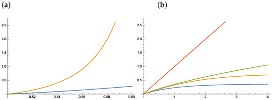
Figure 1. Exact TV distance and the upper bound for (a) TV(Bin$(20,\frac{1}{2})$, Bin$(20,\frac{1}{2}+a))$ and (b) TV(Pois$\left(1\right)$, Pois$(1+a)$). (a) Note that the upper bound becomes useless for $p_2-p_1\ge 0.07$; (b) blue and orange curves – exact TV distance: the blue curve works for $1\le \frac{{\lambda }_2}{{\lambda }_1}\le 2$ and the orange curve for $2\le \frac{{\lambda }_2}{{\lambda }_1}\le 4$. Note that the linear upper bound (red curve) is not relevant and the square root upper (green curve) bound becomes useless for $\frac{{\lambda }_2}{{\lambda }_1}\ge 4$.

Proposition 4 (Distances between exponential distributions). 

(a) Let $X\sim$ Exp$\left(\lambda \right)$, $Y\sim$ Exp$\left(\mu \right)$, $0<\lambda \le \mu <\infty$. Then,

$$\tau (X,Y)={\left(\frac{\lambda }{\mu }\right)}^{\frac{\lambda }{\mu -\lambda }}-{\left(\frac{\lambda }{\mu }\right)}^{\frac{\mu }{\mu -\lambda }}.$$

(23)

(b) Let $\mathbf{X}=(X_1,\dots ,X_d)$, $\mathbf{Y}=(Y_1,\dots ,Y_d)$, each with d i.i.d. components $X_i\sim$ Exp$\left(\lambda \right)$, $Y_i\sim$ Exp$\left(\mu \right)$. Then,

$$\tau (\mathbf{X},\mathbf{Y})={\int }_{z^{*}}^{\infty }({\lambda }^d{e}^{-\lambda y}-{\mu }^d{e}^{-\mu y})\frac{{\left(\sqrt{2}y\right)}^{d-1}}{(d-1)!}\mathrm{d}y$$

(24)

where $z^{*}=\frac{d}{\mu -\lambda }ln\frac{\mu }{\lambda }$.

Proof. 

(a) Indeed, the set $A=\{x>0:\lambda e^{-\lambda x}>\mu e^{-\mu x}\}$ coincides with the half-axis $(y^{*},\infty )$ with $y^{*}=\frac{1}{\mu -\lambda }ln\frac{\mu }{\lambda }$. Consequently, $\tau (\mathbf{X},\mathbf{Y})=e^{-\lambda y^{*}}-e^{-\mu y^{*}}$. (b) In this case, the set $A=\{\mathbf{X}:x_i>0,{\displaystyle \sum _{j=1}^d}{x}_j>z^{*}\}$ with $z^{*}=\frac{d}{\mu -\lambda }ln\frac{\mu }{\lambda }$. Given $y>0$, the area of an $(d-1)$-dimensional simplex $\{\mathbf{x}:x_i>0,{\displaystyle \sum _{j=1}^d}{x}_j=y\}$ equals $\frac{{\left(\sqrt{2}y\right)}^{d-1}}{(d-1)!}$. Then, $\tau (\mathbf{X},\mathbf{Y})={\int }_{\mathbf{x}\in A}[{\displaystyle \prod _{j=1}^d}\lambda e^{-\lambda x_i}-{\displaystyle \prod _{j=1}^d}\mu e^{-\mu x_i}]\mathrm{d}\mathbf{x}$ coincides with (24). □

Proposition 5 (Distances between Poisson distributions). 

Let $X_i\sim$ Po$\left({\lambda }_i\right)$, where $0<{\lambda }_1<{\lambda }_2.$ Then,

$$\tau (X_1,X_2)={\int }_{{\lambda }_1}^{{\lambda }_2}\mathbf{P}(N\left(u\right)=l-1)\mathrm{d}u\le min\left[{\lambda }_2-{\lambda }_1,\sqrt{\frac{2}{e}}(\sqrt{{\lambda }_2}-\sqrt{{\lambda }_1})\right]$$

(25)

where $N\left(u\right)\sim$ Po$\left(u\right)$ and

$$l=l({\lambda }_1,{\lambda }_2)=\lceil ({\lambda }_2-{\lambda }_1){\left(ln\left({\lambda }_2/{\lambda }_1\right)\right)}^{-1}\rceil$$

(26)

with $\lceil {\lambda }_1\rceil \le l\le \lceil {\lambda }_2\rceil$.

Proof. 

Let $N\left(t\right)\sim$ Po$\left(t\right)$; then, via iterated integration by part,

$$\mathbf{P}(N\left(t\right)\le n)=\sum _{k=0}^n{e}^{-t}\frac{t^k}{k!}={\int }_t^{\infty }{e}^{-u}\frac{u^n}{n!}\mathrm{d}u={\int }_t^{\infty }\mathbf{P}(N\left(u\right)=n)\mathrm{d}u.$$

(27)

Hence, Kolm$(X_1,X_2)=\tau (X_1,X_2)=\mathbf{P}(X_2\ge l)-\mathbf{P}(X_1\ge l)=$

$$\mathbf{P}(X_1\le l-1)-\mathbf{P}(X_2\le l-1)={\int }_{{\lambda }_1}^{{\lambda }_2}\mathbf{P}(N\left(u\right)=l-1)\mathrm{d}u$$

where

$$l=min[k\in {\mathbf{Z}}_{+}:f\left(k\right)\ge 1]=\lceil ({\lambda }_2-{\lambda }_1){\left(ln\left({\lambda }_2/{\lambda }_1\right)\right)}^{-1}\rceil$$

and $f\left(k\right)=\frac{\mathbf{P}(N\left({\lambda }_2\right)=k)}{\mathbf{P}(N\left({\lambda }_1\right)=k)}$. □

Proposition 6 (Distances between binomial distributions). 

$X_i\sim$ Bin$(n,p_i)$, $0<p_1<p_2<1$.

$$\tau (X_1,X_2)=n{\int }_{p_1}^{p_2}\mathbf{P}(S_{n-1}\left(u\right)=l-1)\mathrm{d}u\le \frac{\sqrt{e}}{2}\frac{\psi (p_2-p_1)}{{(1-\psi (p_2-p_1))}^2}$$

(28)

where $S_{n-1}\left(u\right)\sim$ Bin$(n-1,u)$ and $\psi \left(x\right)=x\sqrt{\frac{n+2}{2p_1(1-p_1)}}$. Finally, define

$$l=⌈\frac{-nln(1-\frac{p_2-p_1}{1-p_1})}{ln(1+\frac{p_2-p_1}{p_1})-ln(1-\frac{p_2-p_1}{1-p_1}))}⌉$$

(29)

with $\lceil n{p}_1\rceil \le l\le \lceil n{p}_2\rceil$.

Proof. 

Let us prove the following inequality:

$$np\le \frac{-nln(1-x/q)}{ln(1+x/p)-ln(1-x/q)}\le n(p+x),0<x<q$$

(30)

where $p=p_1$, $p+x=p_2$ and $q=1-p$. By concavity of the ln, given $p\in (0,1)$ and $q=1-p$,

$$f\left(x\right)=pln(1+x/p)+qln(1-x/q)\le ln1=0,0<x<q.$$

(31)

This gives the bound $\lceil n{p}_1\rceil \le l$ as follows:

$$\begin{array}{c}pln(1+x/p)+qln(1-x/q)\le 0\Rightarrow npln(1+x/p)-npln(1-x/q)\le -nln(1-x/q)\hfill \\ \Rightarrow np\le \frac{-nln(1-x/q)}{ln(1+x/p)-ln(1-x/q)}.\hfill \end{array}$$

(32)

On the other hand,

$$h\left(x\right)=(p+x)ln(1+x/p)+(q-x)ln(1-x/q)\ge 0,0\le x\le q$$

(33)

as $h\left(0\right)=0$ and $h^{\prime }\left(x\right)=ln(1+x/p-ln(1-x/q)\le 0$; this implies the bound $l\le \lceil n{p}_2\rceil$. Indeed:

$$\begin{array}{c}(p+x)ln(1+x/p)+(q-x)ln(1-x/q)\ge 0\Rightarrow \hfill \\ n(p+x)ln(1+x/p)+n(p+x)ln(1-x/q)\ge -nln(1-x/q)\hfill \\ \Rightarrow n(p+x)\ge \frac{-nln(1-x/q)}{ln(1+x/p)-ln(1-x/q)}.\hfill \end{array}$$

(34)

The rest of the solution goes in parallel with that of Proposition 5. Equation (27) is replaced with the following relation: if $S_n\left(p\right)\sim$ Bin$(n,p)$; then,

$$\mathbf{P}(S_n\left(p\right)\ge k)=n{\int }_0^p\mathbf{P}(S_{n-1}\left(u\right)=k-1)\mathrm{d}u$$

(35)

In fact, iterated integration by parts yields the RHS of (35)

$$\begin{array}{c}=\frac{n(n-1)\dots (n-k+1)}{1\dots k}{p}^k{(1-p)}^{n-k}+\frac{n(n-1)\dots (n-k)}{1\dots (k+1)}{p}^{k+1}{(1-p)}^{n-k+1}\hfill \\ +\dots +p^n=\hfill \end{array}$$

(36)

the LHS of (35). □

Proposition 7 (Distance between binomial and Poisson distributions).

$X\sim$ Bin$(n,p)$ and $Y\sim$ Po$\left(np\right)$, $0<np<2-\sqrt{2}$

$$\tau (X,Y)=np[{(1-p)}^{n-1}-e^{-np}]$$

(37)

Alternative bound

$$\mathrm{TV}(\mathrm{Bin}(n,\frac{\lambda }{n}),\mathrm{Pois}\left(\lambda \right))\le 1-{\left(1-\frac{\lambda }{n}\right)}^{1/2}.$$

(38)

For the sum of Bernoulli r.v.’s $S_n={\displaystyle \sum _{j=1}^n}{X}_j$ with $\mathbf{P}(X_i=1)=p_i$,

$$\tau (S_n,Y_n)=\frac{1}{2}\sum _{k=1}^{\infty }|\mathbf{P}(S_n=k)-\frac{{\lambda }_n^k}{k!}{e}^{-{\lambda }_n}|<\sum _{i=1}^n{p}_i^2$$

(39)

where $Y_n\sim$ Po$\left({\lambda }_n\right)$, ${\lambda }_n=p_1+p_2+\dots +p_n$ (Le Cam). A stronger result: for $X_i\sim$ Bernoulli $\left(p_i\right)$ and $Y_i\sim$ Po$({\lambda }_i=p_i)$, there exists a coupling s.t.

$$\tau (X_i,Y_i)=\mathbf{P}(X_i\ne Y_i)=p_i(1-e^{-p_i}).$$

The stronger form of (39):

$$\frac{1}{32}\left(1\wedge {\lambda }_n^{-1}\right)\sum _{j=1}^n{p}_i^2\le \tau (X_n,Y_n)\le {\lambda }_n^{-1}\left(1-e^{-{\lambda }_n}\right)\sum _{j=1}^n{p}_i^2.$$

(40)

Proposition 8 (Distance between negative binomial distributions).

Let $X_i\sim$ NegBin $(m,p_i)$, $0<p_1<p_2<1$

$$\tau (X_1,X_2)=(m+l-1){\int }_{p_1}^{p_2}\mathbf{P}(S_{m+l-2}\left(u\right)=m-1)\mathrm{d}u$$

(41)

where $S_n\left(u\right)\sim$ Bin$(n,u)$ and

$$l=\lceil -m\frac{ln(1+\frac{p_2-p_1}{p_1})}{ln(1-\frac{p_2-p_1}{1-p_1})}\rceil$$

(42)

with $\lceil m\frac{1-p_2}{p_2}]\le l\le [m\frac{1-p_1}{p_1}\rceil$.

5. Total Variance Distance in the Multi-Dimensional Gaussian Case

Theorem 2.

Let $\tau =\mathrm{TV}(N\left({\mu }_1,{\Sigma }_1),N({\mu }_2,{\Sigma }_2)\right)$, and ${\Sigma }_1,{\Sigma }_2$ be positively definite. Let $\delta ={\mu }_1-{\mu }_2$ and Π be a $d\times (d-1)$ matrix whose columns form a basis for the subspace orthogonal to δ. Let ${\lambda }_1,\dots ,{\lambda }_{d-1}$ denote the eigenvalues of the matrix ${({\Pi }^T{\Sigma }_1\Pi )}^{-1}{\Pi }^T{\Sigma }_2\Pi -{\mathbf{I}}_{d-1}$ and $\lambda =\sqrt{{\displaystyle \sum _{i=1}^{d-1}}{\lambda }_i^2}$. In ${\mu }_1\ne {\mu }_2$, then

$$\frac{1}{200}min[1,\phi (\delta ,{\Sigma }_1,{\Sigma }_2)]\le \tau \le \frac{9}{2}min[1,\phi (\delta ,{\Sigma }_1,{\Sigma }_2)]$$

(43)

where

$$\phi (\delta ,{\Sigma }_1,{\Sigma }_2)=max[\frac{{\delta }^T({\Sigma }_1-{\Sigma }_2)\delta }{{\delta }^T{\Sigma }_1\delta },\frac{\sqrt{{\delta }^T\delta }}{\sqrt{{\delta }^T{\Sigma }_1\delta }},\lambda ]$$

(44)

In the case of equal means ${\mu }_1={\mu }_2$, the bound (43) is simplified:

$$\frac{1}{100}min[1,\lambda ]\le \tau \le \frac{3}{2}min[1,\lambda ].$$

(45)

Here, $\lambda =\sqrt{{\displaystyle \sum _{j=1}^d}{\lambda }_j^2}$, ${\lambda }_1,\dots ,{\lambda }_d$ are the eigenvalues of ${\Sigma }_1^{-1}{\Sigma }_2-{\mathbf{I}}_d$ for positively definite ${\Sigma }_1,{\Sigma }_2$.

Proof is given in Section 6.

Suppose $r\ll d$, and we want to find a low-dimensional projection $A\in {\mathbf{R}}^{r\times d},A{A}^T={\mathbf{I}}_r$ of the multidimensional data $\mathbf{X}\sim$ N$({\mu }_1,{\Sigma }_1)$ and $\mathbf{Y}\sim$ N$({\mu }_2,{\Sigma }_2)$ such that $\mathrm{TV}(A\mathbf{X},A\mathbf{Y})\to max$. The problem may be reduced to the case ${\mu }_1={\mu }_2=0,$ ${\Sigma }_1={\mathbf{I}}_n$, ${\Sigma }_2=\Sigma$, cf. [6]. In view of (44), it is natural to maximize

$$min[1,\sum _{i=1}^{r}g\left({\gamma }_i\right)]$$

(46)

where $g\left(x\right)={\left(\frac{1}{x}-1\right)}^2$ and ${\gamma }_i$ are the eigenvalues of $A\Sigma A^T$. Consider all permutations $\pi$ of these eigenvalues. Let

$${\pi }^{*}={\mathrm{argmax}}_{\pi }\sum _{i=1}^{r}g\left({\lambda }_{\pi \left(i\right)}\right),{\gamma }_i={\lambda }_{{\pi }^{*}\left(i\right)},i=1,\dots ,r.$$

(47)

Then, rows of matrix A should be selected as the normalized eigenvectors of $\Sigma$ associated with the eigenvalues ${\gamma }_i$.

Remark 2.

For zero-mean Gaussian models, this procedure may be repeated mutatis mutandis for any of the so-called f-divergences $D_f\left(\mathbf{P}\right|\left|\mathbf{Q}\right):={\mathbf{E}}_{\mathbf{P}}\left[f\left(\frac{\mathrm{d}\mathbf{Q}}{\mathrm{d}\mathbf{P}}\right)\right]$, where f is a convex function such that $f\left(1\right)=0$, cf. [6]. The most interesting examples are:

(1)

KL-divergence: $f\left(t\right)=tlogt$ and $g\left(x\right)=\frac{1}{2}(x-logx-1)$;

(2)

Symmetric KL-divergence: $f\left(t\right)=(t-1)logt$ and $g\left(x\right)=\frac{1}{2}(x+\frac{1}{x}-2)$;

(3)

The total variance distance: $f\left(t\right)=\frac{1}{2}|t-1|$ and $g\left(x\right)={\left(\frac{1}{x}-1\right)}^2$;

(4)

The square of Hellinger distance: $f\left(t\right)={(\sqrt{t}-1)}^2$ and $g\left(x\right)={\left(\frac{x+1}{x}\right)}^2$;

(5)

${\chi }^2-$divergence: $f\left(t\right)={(t-1)}^2$ and $g\left(x\right)=\frac{1}{\sqrt{x(2-x)}}$.

For the optimization procedure in (47), the following result is very useful.

Theorem 3 (Poincaré Separation Theorem). 

Let Σ be a real symmetric $d\times d$ matrix and A be a semi-orthogonal $r\times d$ matrix. The eigenvalues of Σ (sorted in the descending order) and the eigenvalues of $A\Sigma A^T$ denoted by $\{{\gamma }_i,i=1,\dots ,r\}$ (sorted in the descending order) satisfy

$${\lambda }_{d-(r-i)}\le {\gamma }_i\le {\lambda }_i,i=1,\dots ,r.$$

Proposition 9.

Let $\mathbf{X},\mathbf{Y}$ be two Gaussian PDs with the same covariance matrix: $\mathbf{X}\sim$ N$({\mu }_1,\Sigma )$, $\mathbf{Y}\sim$ N$({\mu }_2,\Sigma )$. Suppose that matrix Σ is non-singular. Then,

$$\tau (\mathbf{X},\mathbf{Y})=2\mathsf{\Phi }\left(\right|\left|{\Sigma }^{-1/2}({\mu }_1-{\mu }_2)\right||/2)-1.$$

(48)

Proof. 

Here, the set $A:=\{\mathbf{x}\in {\mathbf{R}}^d:p\left(\mathbf{x}\right|{\mu }_1,\Sigma )>p\left(\mathbf{x}\right|{\mu }_2,\Sigma )\}$ is a half-space. Indeed,

$$p\left(\mathbf{x}\right|{\mu }_1,\Sigma )>p\left(\mathbf{x}\right|{\mu }_2,\Sigma )\iff 2{\mathbf{x}}^T{\Sigma }^{-1}({\mu }_2-{\mu }_1)<{\mu }_2^T{\Sigma }^{-1}{\mu }_2-{\mu }_1^T{\Sigma }^{-1}{\mu }_1.$$

(49)

After the change of variables $\mathbf{x}\to \mathbf{x}+{\mu }_1$, we need to evaluate the expression

$$\begin{array}{c}I:=\frac{1}{{\left(2\pi \right)}^{d/2}\det {(\Sigma )}^{1/2}}{\int }_{{\mathbf{R}}^d}\mathbf{1}\left({\mathbf{x}}^T{\Sigma }^{-1}\delta <\frac{1}{2}\left|\right|{\Sigma }^{-1/2}\delta {\left|\right|}^2\right)\hfill \\ \times \left(e^{-{\mathbf{x}}^T{\Sigma }^{-1}\mathbf{x}/2}-e^{-{(\mathbf{x}-\delta )}^T{\Sigma }^{-1}(\mathbf{x}-\delta )/2}\right)\mathrm{d}\mathbf{x}.\hfill \end{array}$$

(50)

Take an orthogonal $d\times d$ matrix O such that $O{\Sigma }^{-1/2}\delta =\left|\right|{\Sigma }^{-1/2}\delta \left|\right|e_1$ and change the variables $\mathbf{x}={\Sigma }^{1/2}{O}^T\mathbf{u}$. Then,

$$\begin{array}{c}{\mathbf{x}}^T{\Sigma }^{-1}\delta =\left|\right|{\Sigma }^{-1/2}\delta \left|\right|u_1,{\mathbf{x}}^T{\Sigma }^{-1}\mathbf{x}={\mathbf{u}}^T\mathbf{u},\hfill \\ {(\mathbf{x}-\delta )}^T{\Sigma }^{-1}(\mathbf{x}-\delta )={\mathbf{u}}^T\mathbf{u}+\left|\right|{\Sigma }^{-1/2}{\delta \left|\right|}^2-2\left|\right|{\Sigma }^{-1/2}\delta \left|\right|u_1.\hfill \end{array}$$

(51)

Thus,

$$\begin{array}{c}I=\frac{1}{{\left(2\pi \right)}^{d/2}}{\int }_{{\mathbf{R}}^{d-1}}{e}^{-{\mathbf{v}}^T\mathbf{v}/2}\mathrm{d}\mathbf{v}{\int }_{-\infty }^{\left|\right|{\Sigma }^{-1/2}\delta \left|\right|/2}\left(e^{-u_1^2/2}-e^{-(u_1-\left|\right|{\Sigma }^{-1/2}{\delta \left|\right|)}^2/2}\right)\mathrm{d}{u}_1\hfill \\ =\mathsf{\Phi }\left(b\right)-\mathsf{\Phi }(-b)\hfill \end{array}$$

(52)

where $b=\left|\right|{\Sigma }^{-1/2}\delta \left|\right|/2$. □

6. Proofs for the Multi-Dimensional Gaussian Case

Let $X_i\sim$ N$({\mu }_i,{\Sigma }_i),i=1,2$. W.l.o.g., assume that ${\Sigma }_1,{\Sigma }_2$ are positively definite, and the general case may be followed from the identity

$$\mathrm{TV}(\mathrm{N}(0,{\Sigma }_1),\mathrm{N}(0,{\Sigma }_2))=\mathrm{TV}(\mathrm{N}(0,{\Pi }^T{\Sigma }_1\Pi ),\mathrm{N}(0,{\Pi }^T{\Sigma }_2\Pi ))$$

(53)

where $\Pi$ is $d\times r$ matrix whose columns form an orthogonal basis for range $\left({\Sigma }_{1,2}\right)$. Denote $u=({\mu }_1+{\mu }_2)/2,\delta ={\mu }_1-{\mu }_2$ and decompose $\forall w\in {\mathbf{R}}^d$ as

$$w=u+f_1\left(w\right)\delta +f_2\left(w\right),f_2{\left(w\right)}^T\delta =0.$$

Then,

$$\begin{array}{c}max[\mathrm{TV}(f_1\left(X_1\right),f_1\left(X_2\right)),\mathrm{TV}(f_2\left(X_1\right),f_2\left(X_2\right))]\le \mathrm{TV}(X_1,X_2)\hfill \\ \le \mathrm{TV}(f_1\left(X_1\right),f_1\left(X_2\right))+\mathrm{TV}(f_2\left(X_1\right),f_2\left(X_2\right))\hfill \end{array}$$

(54)

All the components are Gaussian and $f_1\left(X_1\right)\sim$ N$\left(\frac{1}{2},\frac{{\delta }^T{\Sigma }_1\delta }{{\delta }^T\delta }\right)$, $f_1\left(X_2\right)\sim$ N$\left(-\frac{1}{2},\frac{{\delta }^T{\Sigma }_2\delta }{{\delta }^T\delta }\right)$, $f_2\left(X_1\right)\sim$ N$(0,\mathbf{P}{\Sigma }_1\mathbf{P})$, $f_2\left(X_2\right)\sim$ N$(0,\mathbf{P}{\Sigma }_2\mathbf{P})$, $\mathbf{P}={\mathbf{I}}_d-\frac{\delta {\delta }^T}{{\delta }^T\delta }$. We claim that

$$\begin{array}{c}\frac{1}{200}min[1,max[\frac{{\delta }^T({\Sigma }_1-{\Sigma }_2)\delta }{2{\delta }^T{\Sigma }_1\delta },\frac{40\sqrt{{\delta }^T\delta }}{\sqrt{{\delta }^T{\Sigma }_1\delta }}]]\hfill \\ \le \mathrm{TV}(f_1\left(X_1\right),f_1\left(X_2\right))\le \frac{3{\delta }^T({\Sigma }_1-{\Sigma }_2)\delta }{2{\delta }^T{\Sigma }_1\delta }+\frac{\sqrt{{\delta }^T\delta }}{2\sqrt{{\delta }^T{\Sigma }_1\delta }},\hfill \end{array}$$

(55)

$$\frac{1}{100}min[1,\lambda ]\le \mathrm{TV}(f_2\left(X_1\right),f_2\left(X_2\right))\le \frac{3}{2}\lambda$$

(56)

where $\lambda ={\left({\displaystyle \sum _{j=1}^d}{\lambda }_j\right)}^{1/2}$ and ${\lambda }_i$ are the eigenvalues of ${\Sigma }_1^{-1}{\Sigma }_2-{\mathbf{I}}_d$.

Proof of upper bound. 

It follows from Pinsker’s inequality. Let $d=1$ and ${\sigma }_2\ge {\sigma }_1$. Then, for $x=\frac{{\sigma }_2^2}{{\sigma }_1^2}$, we have $x-1-lnx\le {(x-1)}^2$ and, by Pinsker’s inequality,

$$\begin{array}{c}\mathrm{TV}\left(\mathrm{N}({\mu }_1,{\sigma }_1^2),\mathrm{N}({\mu }_2,{\sigma }_2^2)\right)\le \frac{1}{2}\sqrt{\frac{{\sigma }_2^2}{{\sigma }_1^2}-1-ln\frac{{\sigma }_2^2}{{\sigma }_1^2}+\frac{{\Delta }^2}{{\sigma }_1^2}}\hfill \\ \le \frac{1}{2}\sqrt{\frac{{\sigma }_2^2}{{\sigma }_1^2}-1-ln\frac{{\sigma }_2^2}{{\sigma }_1^2}}+\frac{1}{2}\sqrt{\frac{{\Delta }^2}{{\sigma }_1^2}}\le \frac{1}{2}\frac{|{\sigma }_2^2-{\sigma }_1^2|}{{\sigma }_1^2}+\frac{1}{2}\frac{\Delta }{{\sigma }_1}.\hfill \end{array}$$

(57)

For $d>1$, it is enough to obtain the upper bound in the case ${\mu }_1={\mu }_2=0$. Again, Pinsker’s inequality implies: if ${\lambda }_i>-\frac{2}{3}\forall i$,

$$4\mathrm{TV}{\left(\mathrm{N}(0,{\Sigma }_1),\mathrm{N}(0,{\Sigma }_2)\right)}^2\le \sum _{i=1}^d{\lambda }_i-ln(1+{\lambda }_i)\le \sum _{i=1}^d{\lambda }_i^2={\lambda }^2$$

(58)

□

Sketch of proof for lower bound, cf. [7]. 

In a 1D case with $X_i\sim$ N$({\mu }_i,{\sigma }_i^2)$ (${\mu }_1\le {\mu }_2$),

$$\begin{array}{c}\mathrm{TV}(\mathrm{N}({\mu }_1,{\sigma }_1^2),\mathrm{N}({\mu }_2,{\sigma }_2^2))\ge \mathbf{P}(X_2\ge {\mu }_2)-\mathbf{P}(X_1\ge {\mu }_2)=\hfill \\ \frac{1}{2}-\left(\frac{1}{2}-\mathbf{P}(X_1\in ({\mu }_1,{\mu }_2))\right)=\mathbf{P}(X_1\in ({\mu }_1,{\mu }_2))\hfill \\ \ge \frac{1}{5}min[1,\frac{\Delta }{{\sigma }_1}]\hfill \end{array}$$

(59)

Next,

$$\mathrm{TV}(\mathrm{N}({\mu }_1,{\sigma }_1^2),\mathrm{N}({\mu }_2,{\sigma }_2^2))\ge \frac{1}{2}\mathrm{TV}(\mathrm{N}(0,{\sigma }_1^2),\mathrm{N}(0,{\sigma }_2^2))$$

(60)

Indeed, assume w.l.o.g. ${\mu }_1\le {\mu }_2,{\sigma }_1\le {\sigma }_2$. Then, $\exists c=c({\sigma }_1,{\sigma }_2)$:

$$\mathrm{TV}(\mathrm{N}(0,{\sigma }_1^2),\mathrm{N}(0,{\sigma }_2^2))=\mathbf{P}(N(0,{\sigma }_2^2)\notin [-c,c])-\mathbf{P}(N(0,{\sigma }_1^2)\notin [-c,c])$$

Hence,

$$\begin{array}{c}\mathrm{TV}(\mathrm{N}({\mu }_1,{\sigma }_1^2),\mathrm{N}({\mu }_2,{\sigma }_2^2))\ge \mathbf{P}(\mathrm{N}({\mu }_2,{\sigma }_2^2)>c+{\mu }_1)-\mathbf{P}(\mathrm{N}({\mu }_1,{\sigma }_1^2)>c+{\mu }_1)\hfill \\ \ge \frac{1}{2}\mathrm{TV}(\mathrm{N}(0,{\sigma }_1^2),\mathrm{N}(0,{\sigma }_2^2))\hfill \end{array}$$

(61)

Thus, it is enough to study the case ${\mu }_1={\mu }_2=0$. Let $C=\mathrm{diag}(1+{\lambda }_i)$. Then,

$$\mathrm{TV}(\mathrm{N}(0,{\Sigma }_1),\mathrm{N}(0,{\Sigma }_2))=\mathrm{TV}(\mathrm{N}(0,C^{-1}),\mathrm{N}(0,{\mathbf{I}}_d))$$

In the case when there exists i: $|{\lambda }_i|>0.1$,

$$\begin{array}{c}\mathrm{TV}(\mathrm{N}(0,C^{-1}),\mathrm{N}(0,{\mathbf{I}}_d))\ge \mathrm{TV}(\mathrm{N}(0,{(1+{\lambda }_i)}^{-1}),\mathrm{N}(0,1))=\hfill \\ \mathrm{TV}(\mathrm{N}(0,1),\mathrm{N}(0,1+{\lambda }_i))\ge \mathbf{P}(\mathrm{N}(0,1)\in [-1,1])\hfill \\ -\mathbf{P}\left(\mathrm{N}\right(0,1.1)\in [-1,1\left]\right)>0.68-0.66>0.01\hfill \end{array}$$

(62)

Finally, in the case when $|{\lambda }_i|\le 0.1$$\forall i$, the result follows from the lower bound

$$\mathrm{TV}(\mathrm{N}(0,C^{-1}),\mathrm{N}(0,{\mathbf{I}}_d))\ge \frac{\lambda }{6}-\frac{{\lambda }^2}{8}-\frac{1}{2}\left(e^{{\lambda }^2}-1\right)$$

(63)

The bound (63) $>\frac{\lambda }{100}$ if $\lambda <0.17$ and $>0.01$ if $\lambda \ge 0.17$ and $|{\lambda }_i|<0.1\forall i$. We refer to [7] for the proofs of these facts. □

7. Estimation of Lévy–Prokhorov Distance

Let ${\mathbf{P}}_i,i=1,2,$ be probability distributions on a metric space W with metric r. Define the Lévy–Prokhorov distance ${\rho }^{L-P}({\mathbf{P}}_1,{\mathbf{P}}_2)$ between ${\mathbf{P}}_1,{\mathbf{P}}_2$ as the infimum of numbers $ϵ>0$ such that, for any closed set $C\subset W$,

$${\mathbf{P}}_1\left(C\right)-{\mathbf{P}}_2\left(C_{ϵ}\right)<ϵ,{\mathbf{P}}_2\left(C\right)-{\mathbf{P}}_1\left(C_{ϵ}\right)<ϵ$$

(64)

where $C_{ϵ}$ stands for the $ϵ$-neighborhood of C in metric r. It could be checked that ${\rho }^{L-P}({\mathbf{P}}_1,{\mathbf{P}}_2)\le \tau ({\mathbf{P}}_1,{\mathbf{P}}_2)$, i.e., the total variance distance. Equivalently,

$${\rho }^{L-P}({\mathbf{P}}_1,{\mathbf{P}}_2)=\underset{\overline{\mathbf{P}}\in \mathcal{P}({\mathbf{P}}_1,{\mathbf{P}}_2)}{inf}inf[ϵ>0:\mathbf{P}(r(X_1,X_2)>ϵ)<ϵ]$$

(65)

where $\mathcal{P}({\mathbf{P}}_1,{\mathbf{P}}_2)$ is the set of all joint $\overline{\mathbf{P}}$ on $W\times W$ with marginals ${\mathbf{P}}_i$.

Next, define the Wasserstein distance $W_p^r({\mathbf{P}}_1,{\mathbf{P}}_2)$ between ${\mathbf{P}}_1,{\mathbf{P}}_2$ by

$$W_p^r({\mathbf{P}}_1,{\mathbf{P}}_2)=\underset{\overline{\mathbf{P}}\in \mathcal{P}({\mathbf{P}}_1,{\mathbf{P}}_2)}{inf}{\left({\mathbf{E}}_{\overline{\mathbf{P}}}\left[r{(X_1,X_2)}^p\right]\right)}^{1/p}.$$

(66)

In the case of Euclidean space with $r(x_1,x_2)=\left|\right|x_1-x_2\left|\right|$, the index r is omitted.

Total Variation, Wasserstein and Kolmogorov–Smirnov distances defined above are stronger than weak convergence (i.e., convergence in distribution, which is weak* convergence on the space of probability measures, seen as a dual space). That is, if any of these metrics go to zero as $n\to \infty$, then we have weak convergence. However, the converse is not true. However, weak convergence is metrizable (e.g., by the Lévy–Prokhorov metric).

Theorem 4 (Dobrushin’s bound).

$${\rho }^{L-P}({\mathbf{P}}_1,{\mathbf{P}}_2)\le {\left[W_1^r({\mathbf{P}}_1,{\mathbf{P}}_2)\right]}^{1/2}.$$

(67)

Proof. 

Suppose that there exists a closed set C for which at least one of the inequalities (64) fails, say ${\mathbf{P}}_1\left(C\right)\ge ϵ+{\mathbf{P}}_2\left(C_{ϵ}\right)$. Then, for any joint $\overline{\mathbf{P}}$ with marginals ${\mathbf{P}}_1$ and ${\mathbf{P}}_2$,

$$\begin{array}{c}{\mathbf{E}}_{\overline{\mathbf{P}}}\left[r(X_1,X_2)\right]\ge {\mathbf{E}}_{\overline{\mathbf{P}}}\left[\mathbf{1}(r(X_1,X_2)\ge ϵ)r(X_1,X_2)\right]\hfill \\ \ge ϵ\overline{\mathbf{P}}(r(X_1,X_2)\ge ϵ)\ge ϵ\overline{\mathbf{P}}(X_1\in C,X_2\in W\setminus C_{ϵ})\hfill \\ \ge ϵ\left[\overline{\mathbf{P}}(X_1\in C)-\overline{\mathbf{P}}(X_1\in C,X_2\in C_{ϵ})\right]\hfill \\ \ge ϵ\left[\overline{\mathbf{P}}(X_1\in C)-\overline{\mathbf{P}}(X_2\in C_{ϵ})\right]=ϵ\left[{\mathbf{P}}_1(X_1\in C)-{\mathbf{P}}_2(X_2\in C_{ϵ})\right]\ge {ϵ}^2.\hfill \end{array}$$

(68)

This leads to (67), as claimed. □

The Lévy–Prokhorov distance is quite tricky to compute, whereas the Wasserstein distance can be found explicitly in a number of cases. Say, in a 1D case $W={\mathbf{R}}^1$, we have

Theorem 5.

For $d=1$,

$$W_1({\mathbf{P}}_1,{\mathbf{P}}_2)={\int }_{\mathbf{R}}|F_1\left(x\right)-F_2\left(x\right)|\mathrm{d}x.$$

(69)

Proof. 

First, check the upper bound $W_1({\mathbf{P}}_1,{\mathbf{P}}_2)\le {\int }_{\mathbf{R}}|F_1\left(x\right)-F_2\left(x\right)|\mathrm{d}x$. Consider $\xi \sim$ U$[0,1]$, $X_i=F_i^{-1}\left(\xi \right),i=1,2$. Then, in view of the Fubini theorem,

$$\mathbf{E}\left[\right|X_1-X_2\left|\right]={\int }_0^1|F_1^{-1}\left(y\right)-F_2^{-1}\left(y\right)|\mathrm{d}y={\int }_{\mathbf{R}}|F_1\left(x\right)-F_2\left(x\right)|\mathrm{d}x.$$

(70)

For the proof of the inverse inequality, see [8]. □

Proposition 10.

For $d=1$ and $p>1$,

$$\begin{array}{c}{W}_p{({\mathbf{P}}_1,{\mathbf{P}}_2)}^p=p(p-1){\int }_{-\infty }^{\infty }\mathrm{d}y{\int }_y^{\infty }max[F_2\left(y\right)-F_1\left(x\right),0]{(x-y)}^{p-2}\mathrm{d}x\hfill \\ +p(p-1){\int }_{-\infty }^{\infty }\mathrm{d}x{\int }_x^{\infty }max[F_1\left(x\right)-F_2\left(y\right),0]{(y-x)}^{p-2}\mathrm{d}y.\hfill \end{array}$$

(71)

Proof. 

It follows from the identity

$$\begin{array}{c}{\mathbf{E}\left[\right|X-Y|}^p]=p(p-1){\int }_{-\infty }^{\infty }\mathrm{d}y{\int }_y^{\infty }[F_2\left(y\right)-F(x,y)]{(x-y)}^{p-2}\mathrm{d}x\hfill \\ +p(p-1){\int }_{-\infty }^{\infty }\mathrm{d}x{\int }_x^{\infty }[F_1\left(x\right)-F(x,y)]{(y-x)}^{p-2}\mathrm{d}y\hfill \end{array}$$

(72)

The minimum is achieved for $\overline{F}(x,y)=min[F_1\left(x\right),F_2\left(y\right)]$. For an alternative expression (see [9]):

$$W_p{({\mathbf{P}}_1,{\mathbf{P}}_2)}^p={\int }_0^1{|F_1^{-1}\left(t\right)-F_2^{-1}\left(t\right)|}^p\mathrm{d}t.$$

(73)

□

Proposition 11.

Let $(\mathbf{X},\mathbf{Y})\in {\mathbf{R}}^{2d}$ be jointly Gaussian random variables (RVs) with $\mathbf{E}\left[\mathbf{X}\right]={\mu }^X,\mathbf{E}\left[\mathbf{Y}\right]={\mu }^Y$. Then, the Frechet-1 distance

$$\begin{array}{c}{\rho }^{F_1}(\mathbf{X},\mathbf{Y}):=\mathbf{E}\left[{\displaystyle \sum _{j=1}^d}|X_j-Y_j|\right]\hfill \\ ={\displaystyle \sum _{j=1}^d}\left[({\mu }_j^X-{\mu }_j^Y)\left(1-2\mathsf{\Phi }(-\frac{({\mu }_j^X-{\mu }_j^Y)}{{\widehat{\sigma }}_j})\right)+2{\widehat{\sigma }}_j\phi (-\frac{({\mu }_j^X-{\mu }_j^Y)}{{\widehat{\sigma }}_j})\right].\hfill \end{array}$$

(74)

where ${\widehat{\sigma }}_j={\left({\left({\sigma }_j^X\right)}^2+{\left({\sigma }_j^Y\right)}^2-2\mathrm{Cov}(X_j,Y_j)\right)}^{1/2}$, φ and Φ are PDF and CDF of the standard Gaussian RV. Note that, in the case ${\mu }^X={\mu }^Y$, the first term in (74) vanishes, and the second term gives

$${\rho }^{F_1}(\mathbf{X},\mathbf{Y})=\sqrt{\frac{2}{\pi }}\sum _{j=1}^d{\widehat{\sigma }}_j.$$

(75)

We also present expressions for the Frechet-3 and Frechet-4 distances

$$\begin{array}{c}{\rho }^{F_3}(\mathbf{X},\mathbf{Y})={\left({\displaystyle \sum _{j=1}^d}{|X_j-Y_j|}^3\right)}^{1/3}=({\displaystyle \sum _{j=1}^d}{({\mu }_j^X-{\mu }_j^Y)}^3\left(1-2\mathsf{\Phi }(-\frac{({\mu }_j^X-{\mu }_j^Y)}{{\widehat{\sigma }}_j})\right)\hfill \\ +6{({\mu }_j^X-{\mu }_j^Y)}^2{\widehat{\sigma }}_j\phi (-\frac{({\mu }_j^X-{\mu }_j^Y)}{{\widehat{\sigma }}_j})+3{\left({\widehat{\sigma }}_j\right)}^2({\mu }_j^X-{\mu }_j^Y)[1-2\mathsf{\Phi }(-\frac{({\mu }_j^X-{\mu }_j^Y)}{{\widehat{\sigma }}_j})-\hfill \\ 2\frac{({\mu }_j^X-{\mu }_j^Y)}{{\widehat{\sigma }}_j}\phi (-\frac{({\mu }_j^X-{\mu }_j^Y)}{{\widehat{\sigma }}_j})]+2{\left({\widehat{\sigma }}_j\right)}^3\phi (-\frac{({\mu }_j^X-{\mu }_j^Y)}{{\widehat{\sigma }}_j})\left[{\left(\frac{({\mu }_j^X-{\mu }_j^Y)}{{\widehat{\sigma }}_j}\right)}^2+2\right]{)}^{1/3}\hfill \\ {\rho }^{F_4}(\mathbf{X},\mathbf{Y})={\left({\displaystyle \sum _{j=1}^d}{|X_j-Y_j|}^4\right)}^{1/4}={\left({\displaystyle \sum _{j=1}^d}{({\mu }_j^X-{\mu }_j^Y)}^4+6{({\mu }_j^X-{\mu }_j^Y)}^2{\left({\widehat{\sigma }}_j\right)}^2+3{\left({\widehat{\sigma }}_j\right)}^4\right)}^{1/4}.\hfill \end{array}$$

(76)

All of these expressions are minimized when $\mathrm{Cov}(X_j,Y_j),j=1,\dots ,d$ are maximal. However, this fact does not lead immediately to the explicit expressions for Wasserstein’s metrics. The problem here is that the joint covariance matrix ${\Sigma }_{\mathbf{X},\mathbf{Y}}$ should be positively definite. Thus, the straightforward choice $\mathrm{Corr}(X_j,Y_j)=1$ is not always possible; see Theorem 6 below and [10].

[Maurice René Fréchet (1878–1973), a French mathematician, worked in topology, functional analysis, probability theory and statistics. He was the first to introduce the concept of a metric space (1906) and prove the representation theorem in $L_2$ (1907). However, in both cases, the credit was given to other people: Hausdorff and Riesz. Some sources claim that he discovered the Cramér–Rao inequality before anybody else, but such a claim was impossible to verify since lecture notes of his class appeared to be lost. Fréchet worked in several places in France before moving to Paris in 1928. In 1941, he succeeded Borel at the Chair of Calculus of Probabilities and Mathematical Physics in Sorbonne. In 1956, he was elected to the French Academy of Sciences, at the age of 78, which was rather unusual. He influenced and mentored a number of young mathematicians, notably Fortet and Loève. He was an enthusiast of Esperanto; some of his papers were published in this language].

8. Wasserstein Distance in the Gaussian Case

In the Gaussian case, it is convenient to use the following extension of Dobrushin’s bound for $p=2$:

$${\rho }^{L-P}({\mathbf{P}}_1,{\mathbf{P}}_2)\le {\left[W_p({\mathbf{P}}_1,{\mathbf{P}}_2)\right]}^{p/2},p\ge 1.$$

(77)

Theorem 6.

Let ${\mathbf{X}}_i\sim$ N$({\mu }_i,{\Sigma }_i^2),i=1,2,$ be d-dimensional Gaussian RVs. For simplicity, assume that both matrices ${\Sigma }_1^2$ and ${\Sigma }_2^2$ are non-singular (In the general case, the statement holds with ${\Sigma }_1^{-1}$ understood as Moore–Penrose inversion). Then, the $L_2-$Wasserstein distance $W_2({\mathbf{X}}_1,{\mathbf{X}}_2)=W_2(\mathrm{N}({\mu }_1,{\Sigma }_1^2),\mathrm{N}({\mu }_2,{\Sigma }_2^2))$ equals

$$W_2({\mathbf{X}}_1,{\mathbf{X}}_2)={\left[\left|\right|{\mu }_1-{\mu }_2{\left|\right|}^2+\mathrm{tr}\left({\Sigma }_1^2\right)+\mathrm{tr}\left({\Sigma }_2^2\right)-2\mathrm{tr}\left[{\left({\Sigma }_1{\Sigma }_2^2{\Sigma }_1\right)}^{1/2}\right]\right]}^{1/2}$$

(78)

where ${\left({\Sigma }_1{\Sigma }_2^2{\Sigma }_1\right)}^{1/2}$ stands for the positively definite matrix square-root. The value (78) is achieved when ${\mathbf{X}}_2={\mu }_2+A({\mathbf{X}}_1-{\mu }_1)$ where $A={\Sigma }_1^{-1}{\left({\Sigma }_1{\Sigma }_2^2{\Sigma }_1\right)}^{1/2}{\Sigma }_1^{-1}$.

Corollary 1.

Let ${\mu }_1={\mu }_2=0$. Then, for $d=1$, $W_2(X_1,X_2)=|{\sigma }_1-{\sigma }_2|$. For $d=2$,

$$W_2({\mathbf{X}}_1,{\mathbf{X}}_2)={\left[\mathrm{tr}\left({\Sigma }_1^2\right)+\mathrm{tr}\left({\Sigma }_2^2\right)-2{[\mathrm{tr}\left({\Sigma }_1^2{\Sigma }_2^2\right)+2\sqrt{\det \left({\Sigma }_1{\Sigma }_2\right)}]}^{1/2}\right]}^{1/2}.$$

(79)

Note that the expression in (79) vanishes when ${\Sigma }_1^2={\Sigma }_2^2$.

Example 3.

(a) Let $\mathbf{X}\sim$ N$(0,{\Sigma }_X^2)$, $\mathbf{Y}\sim$ N$(0,{\Sigma }_Y^2)$ where ${\Sigma }_X^2={\sigma }_X^2{\mathbf{I}}_d$ and ${\Sigma }_Y^2={\sigma }_Y^2{\mathbf{I}}_d$. Then, $W_2(\mathbf{X},\mathbf{Y})=\sqrt{d}|{\sigma }_X-{\sigma }_Y|$.

• (b) Let $d=2$, $\mathbf{X}\sim$ N$(0,{\Sigma }_X^2)$, $\mathbf{Y}\sim$ N$(0,{\Sigma }_Y^2)$, where ${\Sigma }_X^2={\sigma }_X^2{\mathbf{I}}_2$, ${\Sigma }_Y^2={\sigma }_Y^2\left(\begin{array}{cc}1& \rho \\ \rho & 1\end{array}\right)$ and $\rho \in (-1,1)$. Then,

  $$W_2(\mathbf{X},\mathbf{Y})=2^{1/2}{\left({\sigma }_X^2+{\sigma }_Y^2-{\sigma }_X{\sigma }_Y{\left[2+2{(1-{\rho }^2)}^{1/2}\right]}^{1/2}\right)}^{1/2}.$$
• (c) Let $d=2$, $\mathbf{X}\sim$ N$(0,{\Sigma }_X^2)$, $\mathbf{Y}\sim$ N$(0,{\Sigma }_Y^2)$, where ${\Sigma }_X^2={\sigma }_X^2\left(\begin{array}{cc}1& {\rho }_1\\ {\rho }_1& 1\end{array}\right)$, ${\Sigma }_Y^2={\sigma }_Y^2\left(\begin{array}{cc}1& {\rho }_2\\ {\rho }_2& 1\end{array}\right)$ and ${\rho }_1,{\rho }_2\in (-1,1)$. Then,

  $$W_2(\mathbf{X},\mathbf{Y})=2^{1/2}{\left({\sigma }_X^2+{\sigma }_Y^2-{\sigma }_X{\sigma }_Y{\left[2+2{\rho }_1{\rho }_2+2{(1-{\rho }_1^2)}^{1/2}{(1-{\rho }_2^2)}^{1/2}\right]}^{1/2}\right)}^{1/2}.$$

Note that, in the case ${\rho }_1={\rho }_2$, $W_2(\mathbf{X},\mathbf{Y})=\sqrt{2}|{\sigma }_X-{\sigma }_Y|$ as in (a).

Proof. 

First, reduce to the case ${\mu }_1={\mu }_2=0$ by using the identity $W_2^2({\mathbf{X}}_1,{\mathbf{X}}_2)=\left|\right|{\mu }_1-{\mu }_2{\left|\right|}^2+W_2^2({\xi }_1,{\xi }_2)$ with ${\xi }_i=X_i-{\mu }_i$. Note that the infimum in (19) is always attained on Gaussian measures as $W_2({\mathbf{X}}_1,{\mathbf{X}}_2)$ is expressed in terms of the covariance matrix ${\Sigma }^2={\Sigma }_{X,Y}^2$ only (cf. (81) below). Let us write the covariance matrix in the block form

$${\Sigma }^2=\left(\begin{array}{cc}{\Sigma }_1^2& K\\ K^T& {\Sigma }_2^2\end{array}\right)=\left(\begin{array}{cc}{\Sigma }_1& 0\\ K^T{\Sigma }_1^{-1}& I\end{array}\right)\left(\begin{array}{cc}I& 0\\ 0& S\end{array}\right)\left(\begin{array}{cc}{\Sigma }_1& {\Sigma }_1^{-1}K\\ 0& I\end{array}\right)$$

(80)

where the so-called Shur’s complement $S={\Sigma }_2^2-K^T{\Sigma }_1^{-2}K$. The problem is reduced to finding the matrix K in (80) that minimizes the expression

$${\int }_{{\mathbf{R}}^d\times {\mathbf{R}}^d}\left|\right|\mathbf{x}-{\mathbf{y}\left|\right|}^2\mathrm{d}{\mathbf{P}}_{\mathbf{X},\mathbf{Y}}(\mathbf{x},\mathbf{y})=\mathrm{tr}\left({\Sigma }_1^2\right)+\mathrm{tr}\left({\Sigma }_2^2\right)-2\mathrm{tr}\left(K\right)$$

(81)

subject to a constraint that the matrix ${\Sigma }^2$ in (80) is positively definite. The goal is to check that the minimum (81) is achieved when the Shur’s complement S in (80) equals 0. Consider the fiber ${\sigma }^{-1}\left(S\right)$, i.e., the set of all matrices K such that $\sigma \left(K\right):={\Sigma }_Y^2-K^T{\left({\Sigma }_X^2\right)}^{-1}K=S$. It is enough to check that the maximum value of $\mathrm{tr}\left(K\right)$ on this fiber equals

$$\underset{F\in {\sigma }^{-1}\left(S\right)}{max}\mathrm{tr}\left(K\right)=\mathrm{tr}\left[{\left({\Sigma }_Y({\Sigma }_X^2-S){\Sigma }_Y\right)}^{1/2}\right].$$

(82)

Since the matrix S is positively defined, it is easy to check that the fiber $S=0$ should be selected. In order to establish (82), represent the positively definite matrix ${\Sigma }_Y^2-S$ in the form ${\Sigma }_Y^2-S=U{D}_r^2{U}^T$, where the diagonal matrix $D_r^2=\mathrm{diag}({\lambda }_1^2,\dots ,{\lambda }_r^2,0,\dots ,0)$ and ${\lambda }_i>0$. Next, $U=\left(U_r\right|U_{d-r})$ is the orthogonal matrix of the corresponding eigenvectors. We obtain the following $r\times r$ identity:

$${\left({\Sigma }_X^{-1}K{U}_r{D}_r^{-1}\right)}^T\left({\Sigma }_X^{-1}K{U}_r{D}_r^{-1}\right)={\mathbf{I}}_r.$$

(83)

It means that ${\Sigma }_X^{-1}K{U}_r{D}_r^{-1}=O_r$, an ‘orthogonal’ $d\times r$ matrix, with $O_r^T{O}_r={\mathbf{I}}_r$, and $K={\Sigma }_X{O}_r{D}_r{U}_r^T$. The matrix $O_r$ parametrises the fiber ${\sigma }^{-1}\left(S\right)$. As a result, we have an optimization problem

$$\mathrm{tr}\left(O^{T}M\right)\to max,M={\Sigma }_X{U}_r{D}_r$$

(84)

in a matrix-valued argument $O_r$, subject to the constraint $O_r^T{O}_r={\mathbf{I}}_r$. A straightforward computation gives the answer $\mathrm{tr}\left[{\left(M^{T}M\right)}^{1/2}\right]$, which is equivalent to (82). Technical details can be found in [11,12]. □

Remark 3.

For general zero means RVs $\mathbf{X},\mathbf{Y}\in {\mathbf{R}}^d$ with the covariance matrices ${\Sigma }_i^2,i=1,2$, the following inequality holds [13]:

$$\mathrm{tr}\left({\Sigma }_1^2\right)+\mathrm{tr}\left({\Sigma }_2^2\right)-2\mathrm{tr}\left[{\left({\Sigma }_1{\Sigma }_2^2{\Sigma }_1\right)}^{1/2}\right]\le \mathbf{E}\left[\right||\mathbf{X}-{\mathbf{Y}\left|\right|}^2]\le \mathrm{tr}\left({\Sigma }_1^2\right)+\mathrm{tr}\left({\Sigma }_2^2\right)+2\mathrm{tr}\left[{\left({\Sigma }_1{\Sigma }_2^2{\Sigma }_1\right)}^{1/2}\right].$$

(85)

9. Distance between Distributions of Different Dimensions

For $m\le d$, define a set of matrices with orthonormal rows:

$$O(m,d)=\{V\in {\mathbf{R}}^{m\times d}:V{V}^T={\mathbf{I}}_m\}$$

(86)

and a set of affine maps $\phi :{\mathbf{R}}^d\to {\mathbf{R}}^m$ such that ${\phi }_{V,b}\left(x\right)=Vx+b$.

Definition 1.

For any measures $\mu \in$ M$\left({\mathbf{R}}^m\right)$ and $\nu \in$ M$\left({\mathbf{R}}^d\right)$, the embeddings of μ into ${\mathbf{R}}^d$ are the set of d-dimensional measures ${\mathsf{\Phi }}^{+}(\mu ,d):=\{\alpha \in \mathrm{M}\left({\mathbf{R}}^n\right):{\phi }_{V,\beta }\left(\alpha \right)=\mu \}$ for some $V\in O(m,d),b\in {\mathbf{R}}^m$, and the projections of ν onto ${\mathbf{R}}^m$ are the set of m-dimensional measures ${\mathsf{\Phi }}^{-}(\nu ,m):=\{\beta \in \mathrm{M}\left({\mathbf{R}}^m\right):{\phi }_{V,\beta }\left(\nu \right)=\beta \}$ for some $V\in O(m,d),b\in {\mathbf{R}}^m$.

Given a metric $\kappa$ between measures of the same dimension, define the projection distance $d^{-}(\mu ,\nu ):={inf}_{\beta \in {\mathsf{\Phi }}^{-}(\nu ,m)}\kappa (\mu ,\beta )$ and the embedding distance $d^{+}(\mu ,\nu ):={inf}_{\alpha \in {\mathsf{\Phi }}^{+}(\mu ,d)}$$\kappa (\alpha ,\nu )$. It may be proved [14] that $d^{+}(\mu ,\nu )=d^{-}(\mu ,\nu )$; denote the common value by $\widehat{d}(\mu ,\nu )$.

Example 4.

Let us compute Wasserstein distance between one-dimensional $X\sim$ N$({\mu }_1,{\sigma }^2)$ and d-dimensional $Y\sim$ N$({\mu }_2,\Sigma )$. Denote by ${\lambda }_1\ge {\lambda }_2\ge \dots \ge {\lambda }_d$ the eigenvalues of Σ. Then,

$${\widehat{W}}_2(X,Y)=\left\{\begin{array}{c}\sigma -\sqrt{{\lambda }_1}if\sigma >\sqrt{{\lambda }_1}\hfill \\ 0if\sqrt{{\lambda }_d}\le \sigma \le \sqrt{{\lambda }_1}\hfill \\ \sqrt{{\lambda }_d}-\sigma if\sigma <\sqrt{{\lambda }_d}.\hfill \end{array}\right.$$

(87)

Indeed, in view of Theorem 6, write

$$\begin{array}{c}{\left(W_2^{-}(X,Y)\right)}^2=\underset{{\left|\right|\mathbf{x}\left|\right|}_2=1,b\in \mathbf{R}}{min}\left[\right||{\mu }_1-{\mathbf{x}}^T{\mu }_2-b{\left|\right|}_2^2\hfill \\ +\mathrm{tr}({\sigma }^2+{\mathbf{x}}^T\Sigma \mathbf{x}-2\sigma \sqrt{{\mathbf{x}}^T\Sigma \mathbf{x}})]=\underset{{\left|\right|\mathbf{x}\left|\right|}_2=1}{min}{(\sigma -\sqrt{{\mathbf{x}}^T\Sigma \mathbf{x}})}^2,\hfill \end{array}$$

(88)

and (87) follows.

Example 5 (Wasserstein-2 distance between Dirac measure on ${\mathbf{R}}^{\mathit{m}}$ and a discrete measure on ${\mathbf{R}}^{\mathit{d}}$).

Let $\mathbf{y}\in {\mathbf{R}}^m$ and ${\mu }_1\in$ M$\left({\mathbf{R}}^m\right)$ be the Dirac measure with ${\mu }_1\left(\mathbf{y}\right)=1$, i.e., all mass centered at $\mathbf{y}$. Let ${\mathbf{x}}_1,\dots ,{\mathbf{x}}_k\in {\mathbf{R}}^d$ be distinct points, $p_1,\dots ,p_k\ge 0,p_1+\dots +p_k=0$, and let ${\mu }_2\in$ M$\left({\mathbf{R}}^d\right)$ be the discrete measure of point masses with ${\mu }_2\left({\mathbf{x}}_i\right)=p_i$, $i=1,\dots ,k$. We seek the Wasserstein distance ${\widehat{W}}_2({\mu }_1,{\mu }_2)$ in a closed-form solution. Suppose $m\le d$; then,

$$\begin{array}{c}{\left(W_2^{-}({\mu }_1,{\mu }_2)\right)}^2=\underset{V\in O(m,d)}{inf}\underset{b\in {\mathbf{R}}^m}{inf}{\displaystyle \sum _{i=1}^k}{p}_i\left|\right|V{\mathbf{x}}_i+b-\mathbf{y}{\left|\right|}_2^2\hfill \\ =\underset{V\in O(m,d)}{inf}{\displaystyle \sum _{i=1}^k}{p}_i\left|\right|V{\mathbf{x}}_i-{\displaystyle \sum _{i=1}^k}{p}_{i}V{\mathbf{x}}_i{\left|\right|}_2^2=\underset{V\in O(m,d)}{inf}\mathrm{tr}\left(VC{V}^T\right)\hfill \end{array}$$

(89)

noting that the second infimum is attained by $b=\mathbf{y}-{\displaystyle \sum _{i=1}^k}{p}_{i}V{\mathbf{x}}_i$ and defining C in the last infimum to be

$$C:=\sum _{i=1}^k{p}_i\left({\mathbf{x}}_i-\sum _{i=1}^k{p}_i{\mathbf{x}}_i\right){\left({\mathbf{x}}_i-\sum _{i=1}^k{p}_i{\mathbf{x}}_i\right)}^T\in {\mathbf{R}}^{d\times d}.$$

(90)

Let the eigenvalue decomposition of the symmetric positively semidefinite matrix C be $C=Q\mathsf{\Lambda }{Q}^T$ with $\mathsf{\Lambda }=\mathrm{diag}({\lambda }_1,\dots ,{\lambda }_d)$, ${\lambda }_1\ge \dots \ge {\lambda }_d\ge 0.$ Then,

$$\underset{V\in O(m,d)}{inf}\mathrm{tr}\left(VC{V}^T\right)=\sum _{i=0}^{m-1}{\lambda }_{d-i}$$

(91)

and is attained when $V\in$ O$(m,d)$ has row vectors given by the last m columns of $Q\in$ O$\left(d\right)$.

Note that the geodesic distance (7) and (8) between Gaussian PDs (or corresponding covariance matrices) is equivalent to the formula for the Fisher information metric for the multivariate normal model [15]. Indeed, the multivariate normal model is a differentiable manifold, equipped with the Fisher information as a Riemannian metric; this may be used in statistical inference.

Example 6.

Consider i.i.d. random variables $Z_l,\dots ,Z_n$ to be bi-variately normally distributed with diagonal covariance matrices, i.e., we focus on the manifold $M_{diag}=\{\mathrm{N}(\mu ,\mathsf{\Lambda }):\mu \in {\mathbf{R}}^2,\mathsf{\Lambda }\mathrm{diagonal}\}$. In this manifold, consider the submodel $M_{diag}^{*}=\{\mathrm{N}(\mu ,{\sigma }^2\mathbf{I}):\mu \in {\mathbf{R}}^2,{\sigma }^2\in {\mathbf{R}}_{+}\}$ corresponding to the hypothesis $H_0:{\sigma }_1^2={\sigma }_2^2$. First, consider the standard statistical estimates $\overline{Z}$ for the mean and $s_1,s_2$ for the variances. If ${\overline{\sigma }}^2$ denotes the geodesic estimate of the common variance, the squared distance between the initial estimate and the geodesic estimate under the hypothesis $H_0$ is given by

$$\frac{n}{2}\left[{\left(ln\frac{{\overline{\sigma }}^2}{s_1^2}\right)}^2+{\left(ln\frac{{\overline{\sigma }}^2}{s_2^2}\right)}^2\right]$$

(92)

which is minimized by ${\overline{\sigma }}^2=s_1{s}_2$. Hence, instead of the arithmetic mean of the initial standard variation estimates, we use as an estimate the geometric mean of these quantities.

Finally, we present the distance between the symmetric positively definite matrices of different dimensions. Let $m\le d$, A is $m\times m$ and $B=\left(\begin{array}{cc}{B}_{11}& B_{12}\\ B_{21}& B_{22}\end{array}\right)$ is $d\times d$; here, $B_{11}$ is a $m\times m$ block. Then, the distance is defined as follows:

$$d_2(A,B):={\left(\sum _{j=1}^m{\left(max[0,ln{\lambda }_j\left(A^{-1}{B}_{11}\right)]\right)}^2\right)}^{1/2}.$$

(93)

In order to estimate the distance (93), after the simultaneous diagonalization of matrices A and B, the following classical result is useful:

Theorem 7 (Cauchy interlacing inequalities).

Let $B=\left(\begin{array}{cc}{B}_{11}& B_{12}\\ B_{21}& B_{22}\end{array}\right)$ be a $d\times d$ symmetric positively definite matrix with eigenvalues ${\lambda }_1\left(B\right)\le \dots \le {\lambda }_d\left(B\right)$ and $m\times m$ block $B_{11}$. Then,

$${\lambda }_j\left(B\right)\le {\lambda }_j\left(B_{11}\right)\le {\lambda }_{j+d-m}\left(B\right),j=1,\dots ,m.$$

(94)

10. Context-Sensitive Probability Metrics

The weighted entropy and other weighted probabilistic quantities generated a substantial amount of literature (see [16,17] and the references therein). The purpose was to introduce a disparity between outcomes of the same probability: in the case of a standard entropy, such outcomes contribute the same amount of information/uncertainty, which is appropriate in context-free situations. However, imagine two equally rare medical conditions, occurring with probability $p\ll 1$, one of which carries a major health risk while the other is just a peculiarity. Formally, they provide the same amount of information: $-logp$, but the value of this information can be very different. The applications of the weighted entropy to the clinical trials are in the process of active development (see [18] and the literature cited therein). In addition, the contribution to the distance (say, from a fixed distribution $\mathbf{Q}$) related to these outcomes, is the same in any conventional sense. The weighted metrics, or weight functions, are supposed to fulfill the task of samples graduation, at least to a certain extent.

Let the weight function or graduation $\phi >0$ on the phase space $\mathcal{X}$ be given. Define the total weighted variation (TWV) distance

$${\tau }_{\phi }({\mathbf{P}}_1,{\mathbf{P}}_2)=\frac{1}{2}\left(\underset{A}{sup}[{\int }_A\phi \mathrm{d}{\mathbf{P}}_1-{\int }_A\phi \mathrm{d}{\mathbf{P}}_2]+\underset{A}{sup}[{\int }_A\phi \mathrm{d}{\mathbf{P}}_2-{\int }_A\phi \mathrm{d}{\mathbf{P}}_1]\right).$$

(95)

Similarly, define the weighted Hellinger distance. Let $p_1,p_2$ be the densities of ${\mathbf{P}}_1,{\mathbf{P}}_2$ w.r.t. to a measure $\nu$. Then,

$${\eta }_{\phi }({\mathbf{P}}_1,{\mathbf{P}}_2):=\frac{1}{\sqrt{2}}{\left(\int \phi {(\sqrt{p_1}-\sqrt{p_2})}^2\mathrm{d}\nu \right)}^{1/2}.$$

(96)

Lemma 1.

Let $p_1,p_2$ be the densities of ${\mathbf{P}}_1,{\mathbf{P}}_2$ w.r.t. to a measure ν. Then, ${\tau }_{\phi }({\mathbf{P}}_1,{\mathbf{P}}_2)$ is a distance and

$${\tau }_{\phi }({\mathbf{P}}_1,{\mathbf{P}}_2)=\frac{1}{2}\int \phi |p_1-p_2|\mathrm{d}\nu$$

(97)

Proof. 

The triangular inequality and other properties of the distance follow immediately. Next,

$$\begin{array}{c}{\int }_{p_1>p_2}\phi (p_1-p_2)=\frac{1}{2}(\int \phi p_1-\int \phi p_2)+\frac{1}{2}\int \phi |p_1-p_2|\mathrm{d}\nu \hfill \\ {\int }_{p_2>p_1}\phi (p_2-p_1)=\frac{1}{2}(\int \phi p_2-\int \phi p_1)+\frac{1}{2}\int \phi |p_1-p_2|\mathrm{d}\nu \hfill \end{array}$$

(98)

Summing up these equalities implies (97). □

Let $\int \phi p_1\mathrm{d}\nu \ge \int \phi p_2\mathrm{d}\nu$. Then, by the weighted Gibbs inequality [16], ${\mathrm{KL}}_{\phi }({\mathbf{P}}_1\left|\right|{\mathbf{P}}_2):=\int \phi p_{1}log\frac{p_1}{p_2}\ge 0$.

Theorem 8 (Weighted Pinsker’s inequality).

$$\frac{1}{2}\int \phi |p_1-p_2|\le \sqrt{{\mathrm{KL}}_{\phi }({\mathbf{P}}_1\left|\right|{\mathbf{P}}_2)/2}\sqrt{\int \phi p_1}.$$

(99)

Proof. 

Define the function $G\left(x\right)=xlogx-x+1$. The following bound holds, cf. (12):

$$G\left(x\right)=xlogx-x+1\ge \frac{3}{2}\frac{{(x-1)}^2}{x+2},x>0.$$

(100)

Now, by the Cauchy–Schwarz inequality,

$$\begin{array}{c}{\left(\int \phi p_2|\frac{p_1}{p_2}-1|\right)}^2\le \int \phi \frac{{(\frac{p_1}{p_2}-1)}^2}{\frac{p_1}{p_2}+2}{p}_2\int \phi \left(\frac{p_1}{p_2}+2\right)p_2\hfill \\ \le 3\int \phi \frac{{(\frac{p_1}{p_2}-1)}^2}{\frac{p_1}{p_2}+2}{p}_2\int \phi p_1\le 2\int \phi G\left(\frac{p_1}{p_2}\right)p_2\int \phi p_1\le {\mathrm{KL}}_{\phi }({\mathbf{P}}_1\left|\right|{\mathbf{P}}_2)\int \phi p_1.\hfill \end{array}$$

(101)

□

Theorem 9 (Weighted Le Cam’s inequality).

$${\tau }_{\phi }({\mathbf{P}}_1,{\mathbf{P}}_2)\ge {\eta }_{\phi }{({\mathbf{P}}_1,{\mathbf{P}}_2)}^2.$$

(102)

Proof. 

In view of inequality

$$\frac{1}{2}|p_1-p_2|=\frac{1}{2}{p}_1+\frac{1}{2}{p}_2-min[p_1,p_2]\ge \frac{1}{2}{p}_1+\frac{1}{2}{p}_2-\sqrt{p_1{p}_2},$$

one obtains

$${\tau }_{\phi }({\mathbf{P}}_1,{\mathbf{P}}_2)\ge \frac{1}{2}\int \phi p_1+\frac{1}{2}\int \phi p_2-\int \phi \sqrt{p_1{p}_2}={\eta }_{\phi }{({\mathbf{P}}_1,{\mathbf{P}}_2)}^2.$$

(103)

□

Next, we relate TWV distance to the sum of sensitive errors of both types in statistical estimation. Let C be the critical domain for the checking the hypothesis $H_1$:${\mathbf{P}}_1$ versus the alternative $H_2$:${\mathbf{P}}_2$. Define by ${\alpha }_{\phi }={\int }_C\phi p_1$ and ${\beta }_{\phi }={\int }_{\mathcal{X}\setminus C}\phi p_2$ the weighted error probabilities of the I and II types.

Lemma 2.

Let $d=d_C$ be the decision rule with the critical domain C. Then,

$$\underset{d}{inf}[{\alpha }_{\phi }+{\beta }_{\phi }]=\frac{1}{2}\left[\int \phi \mathrm{d}{\mathbf{P}}_1+\int \phi \mathrm{d}{\mathbf{P}}_2\right]-{\tau }_{\phi }({\mathbf{P}}_1,{\mathbf{P}}_2).$$

(104)

Proof. 

Denote $C^{*}=\{x:p_2\left(x\right)>p_1\left(x\right)\}$. Then, the result follows from the equality $\forall C$

$$\begin{array}{c}{\int }_C\phi \mathrm{d}{\mathbf{P}}_1+{\int }_{\mathcal{X}\setminus C}\phi \mathrm{d}{\mathbf{P}}_2=\frac{1}{2}\left[\int \phi \mathrm{d}{\mathbf{P}}_1+\int \phi \mathrm{d}{\mathbf{P}}_2\right]\hfill \\ +\int \phi |p_1-p_2|\left[\mathbf{1}(x\in C\cap \mathcal{X}\setminus C^{*})-\mathbf{1}(x\in C\cap C^{*})\right].\hfill \end{array}$$

(105)

□

Theorem 10 (Weighted Fano’s inequality).

Let ${\mathbf{P}}_1,\dots ,{\mathbf{P}}_M$, $M\ge 2$ be probability distributions such that ${\mathbf{P}}_j\ll {\mathbf{P}}_k$, $\forall j,k$. Then,

$$\begin{array}{c}\underset{d}{inf}\underset{1\le j\le M}{max}\int \phi \left(x\right)\mathbf{1}(d\left(x\right)\ne j)\mathrm{d}{\mathbf{P}}_j\left(x\right)\ge \frac{log\left(M\right)}{log(M-1)}\frac{1}{M}{\displaystyle \sum _{j=1}^M}\int \phi p_j\hfill \\ -\frac{1}{log(M-1)}\left[\frac{1}{M^2}{\displaystyle \sum _{j,k=1}^M}{\mathrm{KL}}_{\phi }({\mathbf{P}}_j,{\mathbf{P}}_k)+log2\frac{1}{M}{\displaystyle \sum _{j=1}^M}\int \phi p_j\right]\hfill \end{array}$$

(106)

where the infimum is taken over all tests with values in $\{1,\dots ,M\}$.

Proof. 

Let $Z\in \{1,\dots ,M\}$ be a random variable such that $\mathbf{P}(Z=i)=\frac{1}{M}$ and let $X\sim {\mathbf{P}}_Z$. Note that ${\mathbf{P}}_Z$ is a mixture distribution so that, for any measure $\nu$ such that ${\mathbf{P}}_Z\ll \nu$, we have $\frac{\mathrm{d}{\mathbf{P}}_Z}{\mathrm{d}\nu }=\frac{1}{M}{\displaystyle \sum _{k=1}^M}\frac{\mathrm{d}{\mathbf{P}}_j}{\mathrm{d}\nu }$ and so

$$\mathbf{P}(Z=j|X=x)=\mathrm{d}{\mathbf{P}}_j\left(x\right){\left(\sum _{k=1}^M\mathrm{d}{\mathbf{P}}_k\left(x\right)\right)}^{-1}.$$

It implies by Jensen’s inequality applied to the convex function $-logx$

$$\begin{array}{c}\int \phi \left(x\right){\displaystyle \sum _{j=1}^M}\mathbf{P}(Z=j|X=x)log\mathbf{P}(Z=j|X=x)\mathrm{d}{\mathbf{P}}_X\left(x\right)\hfill \\ \le \frac{1}{M^2}{\displaystyle \sum _{j,k=1}^M}\int \phi log\left(\frac{\mathrm{d}{\mathbf{P}}_j}{\mathrm{d}{\mathbf{P}}_k}\right)\mathrm{d}{P}_j-log\left(M\right)\frac{1}{M}{\displaystyle \sum _{j=1}^M}\int \phi p_j\hfill \\ ={\displaystyle \sum _{j,k=1}^M}{\mathrm{KL}}_{\phi }({\mathbf{P}}_j,{\mathbf{P}}_k)-log\left(M\right)\frac{1}{M}{\displaystyle \sum _{j=1}^M}\int \phi p_j.\hfill \end{array}$$

(107)

On the other hand, denote by $q_j=\frac{\mathbf{P}(Z=j|X)}{\mathbf{P}(Z\ne d(X\left)\right|X)}$ and $h\left(x\right)=xlogx+(1-x)log(1-x)$. Note that $h\left(x\right)\ge -log2$ and by Jensen’s inequality ${\sum }_{j\ne d\left(X\right)}{q}_{j}log{q}_j\ge -log(M-1)$. The following inequality holds:

$$\begin{array}{c}{\displaystyle \sum _{j=1}^M}\mathbf{P}(Z=j|X)log\mathbf{P}(Z=j|X)\hfill \\ =\left(1-\mathbf{P}(Z\ne d(X\left)\right|X)\right)log\left(1-\mathbf{P}(Z\ne d(X\left)\right|X)\right)+{\displaystyle \sum _{j\ne d\left(X\right)}}\mathbf{P}(Z=j|X)log\mathbf{P}(Z=j|X)\hfill \\ =h\left(\mathbf{P}(Z=d\left(X\right)|X)\right)+\mathbf{P}(Z\ne d\left(X\right)|X){\displaystyle \sum _{j\ne d\left(X\right)}}{q}_{j}log{q}_j\hfill \\ \ge -log2-log(M-1)\mathbf{P}\left(d\right(X)\ne Z|X).\hfill \end{array}$$

(108)

Integration of (108) yields

$$\begin{array}{c}\int \phi \left(x\right){\displaystyle \sum _{j=1}^M}\mathbf{P}(Z=j|X=x)log\mathbf{P}(Z=j|X=x)\mathrm{d}{\mathbf{P}}_X\left(x\right)\hfill \\ \ge \left(-log2\frac{1}{M}{\displaystyle \sum _{j=1}^M}\int \phi p_j-log(M-1)\underset{1\le j\le M}{max}\int \phi \left(x\right)\mathbf{1}(d\left(x\right)\ne j)\mathrm{d}{\mathbf{P}}_j\right).\hfill \end{array}$$

(109)

Combining (107) and (109) proves (106). □

11. Conclusions

The contribution of the current paper is summarized in the Table 1 below. The objects 1–8 belong to the treasures of probability theory and statistics, and we present a number of examples and additional facts that are not easy to find in the literature. The objects 9–10, as well as the distances between distributions of different dimensions, appeared quite recently. They are not fully studied and quite rarely used in applied research. Finally, objects 11–12 have been recently introduced by the author and his collaborators. This is the field of the current and future research.

Table 1. The main metrics and divergencies.

Number	Name	Reference	Comment
1	Kullback–Leibler	(2)	Divergence but not a distance
2	Total variation (TV)	(1)	Bounded by Pinsker’s inequality
3	Kolmogorov–Smirnov	p. 2	Specific for 1D case
4	Hellinger	(16)	Bounded by Le Cam’s inequality
5	Lévy–Prohorov	(1)	Metrization of the weak convergence
6	Fréchet	(8, 80)	Requires the joint distribution
7	Wasserstein	(69)	Marginal distributions only
8	${\chi }^2$	p. 5	Divergence but not a distance
9	Jensen–Shannon	(6)	Constructed from Kullback–Leibler
10	Geodesic	(8)	Specific for Gaussian case
11	Weighted TV	(97)	Context sensitive
12	Weighted Hellinger	(98)	Context sensitive

References

- Suhov, Y.; Kelbert, M. Probability and Statistics by Example: Volume I. Basic Probability and Statistics; Second Extended Edition; Cambridge University Press: Cambridge, UK, 2014; 457p. [Google Scholar]
- Rachev, S.T. Probability Metrics and the Stability of Stochastic Models; Wiley: New York, NY, USA, 1991. [Google Scholar]
- Zeifman, A.; Korolev, V.; Sipin, A. (Eds.) Stability Problems for Stochastic Models: Theory and Applications; MDPI: Basel, Switzerland, 2020. [Google Scholar]
- Endres, D.M.; Schindelin, J.E. A new metric for probability distributions. IEEE Trans. Inf. Theory 2003, 49, 1858–1860. [Google Scholar] [CrossRef]
- Kelbert, M.; Suhov, Y. What scientific folklore knows about the distances between the most popular distributions. Izv. Sarat. Univ. (N.S.) Ser. Mat. Mekh. Inform. 2022, 22, 233–240. [Google Scholar] [CrossRef]
- Dwivedi, A.; Wang, S.; Tajer, A. Discriminant Analysis under f-Divergence Measures. Entropy 2022, 24, 188. [Google Scholar] [CrossRef] [PubMed]
- Devroye, L.; Mehrabian, A.; Reddad, T. The total variation distance between high-dimensional Gaussians. arXiv 2020, arXiv:1810.08693v5. [Google Scholar]
- Vallander, S.S. Calculation of the Wasserstein distance between probability distributions on the line. Theory Probab. Appl. 1973, 18, 784–786. [Google Scholar] [CrossRef]
- Rachev, S.T. The Monge-Kantorovich mass transference problem and its stochastic applications. Theory Probab. Appl. 1985, 29, 647–676. [Google Scholar] [CrossRef]
- Gelbrich, M. On a formula for the L2 Wasserstein metric between measures on Euclidean and Hilbert spaces. Math. Nachrichten 1990, 147, 185–203. [Google Scholar] [CrossRef]
- Givens, R.M.; Shortt, R.M. A class of Wasserstein metrics for probability distributions. Mich. Math J. 1984, 31, 231240. [Google Scholar] [CrossRef]
- Olkin, I.; Pwelsheim, F. The distances between two random vectors with given dispersion matrices. Lin. Algebra Appl. 1982, 48, 267–2263. [Google Scholar] [CrossRef]
- Dowson, D.C.; Landau, B.V. The Fréchet distance between multivariate Normal distributions. J. Multivar. Anal. 1982, 12, 450–456. [Google Scholar] [CrossRef]
- Cai, Y.; Lim, L.-H. Distances between probability distributions of different dimensions. IEEE Trans. Inf. Theory 2022, 68, 4020–4031. [Google Scholar] [CrossRef]
- Skovgaard, L.T. A Riemannian geometry of the multivariate normal model. Scand. J. Stat. 1984, 11, 211–223. [Google Scholar]
- Stuhl, I.; Suhov, Y.; Yasaei Sekeh, S.; Kelbert, M. Basic inequalities for weighted entropies. Aequ. Math. 2016, 90, 817–848. [Google Scholar]
- Stuhl, I.; Kelbert, M.; Suhov, Y.; Yasaei Sekeh, S. Weighted Gaussian entropy and determinant inequalities. Aequ. Math. 2022, 96, 85–114. [Google Scholar] [CrossRef]
- Kasianova, K.; Kelbert, M.; Mozgunov, P. Response-adaptive randomization for multi-arm clinical trials using context-dependent information measures. Comput. Stat. Data Anal. 2021, 158, 107187. [Google Scholar] [CrossRef] [PubMed]
Disclaimer/Publisher’s Note: The statements, opinions and data contained in all publications are solely those of the individual author(s) and contributor(s) and not of MDPI and/or the editor(s). MDPI and/or the editor(s) disclaim responsibility for any injury to people or property resulting from any ideas, methods, instructions or products referred to in the content. |
© 2023 by the author. Licensee MDPI, Basel, Switzerland. This article is an open access article distributed under the terms and conditions of the Creative Commons Attribution (CC BY) license (https://creativecommons.org/licenses/by/4.0/).