Ball Comparison between Two Efficient Weighted-Newton-like Solvers for Equations

Abstract

We compare the convergence balls and the dynamical behaviors of two efficient weighted-Newton-like equation solvers by Sharma and Arora, and Grau-Sánchez et al. First of all, the results of ball convergence for these algorithms are established by employing generalized Lipschitz constants and assumptions on the first derivative only. Consequently, outcomes for the radii of convergence, measurable error distances and the existence–uniqueness areas for the solution are discussed. Then, the complex dynamical behaviors of these solvers are compared by applying the attraction basin tool. It is observed that the solver suggested by Grau-Sánchez et al. has bigger basins than the method described by Sharma and Arora. Lastly, our ball analysis findings are verified on application problems and the convergence balls are compared. It is found that the method given by Grau-Sánchez et al. has larger convergence balls than the solver of Sharma and Arora. Hence, the solver presented by Grau-Sánchez et al. is more suitable for practical application. The convergence analysis uses the first derivative in contrast to the aforementioned studies, utilizing the seventh derivative not on these methods. The developed process can be used on other methods in order to increase their applicability.

1. Introduction

Let us consider two Banach spaces $U_1$ and $U_2$. Suppose $V(\ne \varnothing )$ is a subset of $U_1$, which is convex and open. We denote the set {$B_L:U_1\to U_2$ linear and bounded operators} by $L(U_1,U_2)$. For a Fréchet derivable operator $D:V\subseteq U_1\to U_2$, define the equation

$$D\left(a\right)=0.$$

(1)

This equation regularly appears when physical, chemical and other scientific problems are modeled mathematically and we need numerical methods to solve them. Take note that this is a critical job since analytical solutions to these equations are occasionally available. Therefore, nonlinear equations are usually approached by an iterative method, through which an approximate solution can be found. Developing more accurate iterative approaches for approximating the solution of these equations is a huge challenge in general. The conventional Newton’s iterative approach is the most often employed technique for this problem. Besides this, a number of algorithms have been suggested to boost the convergence rate of the orthodox solvers such as Newton’s [1] and Chebyshev–Halley’s [2], among others. Cordero and Torregrosa [3] proposed several variants of Newton’s solver of second, third and fifth convergence orders based on quadrature rules of fifth order for solving nonlinear equations. Two families of zero-finding iterative approaches to address nonlinear equations are presented in [4] by applying Obreshkov-like techniques [5] and Hueso et al. [6] developed a third-order and fourth-order class of predictor–corrector algorithms free from the second derivative to solve systems of nonlinear equations. By composing two weighted-Newton steps, Sharma et al. [6] constructed an efficient fourth-order weighted-Newton method to solve nonlinear systems. Cordero et al. [7] studied two bi-parametric fourth-order families of predictor–corrector iterative solvers by generalizing Ostrowski’s and Chun’s algorithms [8,9]. They used Newton’s solver as the predictor of the first family, and Steffensen’s method as the predictor of the second one. For solving systems of nonlinear equations, Sharma and Arora [10] designed Newton-like iterative approaches of the fifth and eighth orders of convergence.

In this study, we are interested in two sixth convergence order equation solvers proposed by Sharma and Arora [11] and Grau-Sánchez et al. [12], respectively. For a starting point $a_0\in V$, the iterative formula designed by Sharma and Arora is written as follows:

$$\begin{array}{cc}\hfill b_n& =a_n-D^{\prime }{\left(a_n\right)}^{-1}D\left(a_n\right),\hfill \\ \hfill z_n& =b_n-(3I-2D^{\prime }{\left(a_n\right)}^{-1}[a_n,b_n;D])D^{\prime }{\left(a_n\right)}^{-1}D\left(b_n\right),\hfill \\ \hfill a_{n+1}& =z_n-(3I-2D^{\prime }{\left(a_n\right)}^{-1}[a_n,b_n;D])D^{\prime }{\left(a_n\right)}^{-1}D\left(z_n\right).\hfill \end{array}$$

(2)

The solver constructed by Grau-Sánchez et al. can be presented as

$$\begin{array}{cc}\hfill b_n& =a_n-D^{\prime }{\left(a_n\right)}^{-1}D\left(a_n\right),\hfill \\ \hfill z_n& =b_n-A_n^{-1}D\left(b_n\right),\hfill \\ \hfill a_{n+1}& =z_n-A_n^{-1}D\left(z_n\right),\hfill \end{array}$$

(3)

where $a_0\in V$ is a starter, $A_n=2[b_n,a_n;D^{\prime }]-D^{\prime }\left(a_n\right),[.,.;D]:V\times V\to L(U_1,U_2)$. For these iterative procedures, the convergence theorems have been developed by applying the expensive Taylor’s formula and imposing constraints on the derivative of the seventh order. The scope of utilization of these solvers is restricted due to such convergence results based on derivatives of higher order. To demonstrate this, we choose

$$D\left(a\right)=\left\{\begin{array}{cc}{a}^{3}ln\left(a^2\right)+a^5-a^4,\hfill & \mathrm{if}a\ne 0\hfill \\ 0,\hfill & \mathrm{if}a=0\hfill \end{array}\right.,$$

(4)

where $U_1=U_2=\mathbb{R}$ and D is defined on $V=[-\frac{1}{2},\frac{3}{2}]$. Then, it is noteworthy that the existing convergence theorems for (2) and (3) do not hold for this example, since $D^{‴}$ is unbounded on V. In addition, these convergence results produce no statements on $\parallel a_n-a_{\ast }\parallel$, the convergence ball and the precise location of $a_{\ast }$. The ball analysis of an iterative formula is useful in the estimation of the radii of convergence balls and bounds on $\parallel a_n-a_{\ast }\parallel$, and in determining the area of uniqueness for $a_{\ast }$. It should be noted that the effects of ball convergence are extremely beneficial because they shed light on the challenging issue of selecting starting guesses. This motivates us to establish ball convergence of solvers (2) and (3) by applying conditions only on $D^{\prime }$. Our work allows computation of the convergence radii and the estimates $\parallel a_n-a_{\ast }\parallel$, and also provides an accurate location of $a_{\ast }$.

The summary of the entire document can be written as follows: Section 1 is the introduction. The results of ball convergence for solvers (2) and (3) are established in Section 2. Section 3 deals with the comparison of attraction basins for these algorithms. In Section 4, numerical studies are performed. Finally, concluding remarks are written.

2. Ball Analysis

First, it is convenient for the local convergence analysis of solver (2) to develop real parameters and functions. Let $M=[0,\infty )$. Suppose the following:

(1)

Function ${\Gamma }_0\left(h\right)-1$ has a least root $r_0\in M \backslash \left\{0\right\}$ for some function ${\Gamma }_0:M\to M$ that is non-decreasing and continuous. Set $M_0=[0,r_0)$.

(2)

Function $E_1\left(h\right)-1$ has a least root ${\rho }_1\in M_0 \backslash \left\{0\right\}$ for some function $\Gamma :[0,2r_0)\to M$ that is non-decreasing and continuous, and $E_1:M_0\to M$ is defined as

$$E_1\left(h\right)=\frac{{\int }_0^1\Gamma \left((1-\lambda )h\right)d\lambda }{1-{\Gamma }_0\left(h\right)}.$$

(3)

Function ${\Gamma }_0\left(E_1\left(h\right)h\right)-1$ has a least root $r_1\in M_0 \backslash \left\{0\right\}$.

Set $r_2=min\{r_0,r_1\}$ and $M_1=[0,r_2)$.

(4)

Function $E_2\left(h\right)-1$ has a least root ${\rho }_2\in M_1 \backslash \left\{0\right\}$ for some functions ${\Gamma }_1:M_1\to M$, ${\Gamma }_2:M_1\times M_1\to M$ that is non-decreasing and continuous, with function $E_2:M_1\to M$ defined as

$$\begin{array}{c}\hfill E_2\left(h\right)=[E_1\left(E_1\left(h\right)\right)+\frac{({\Gamma }_0\left(h\right)+{\Gamma }_0\left(E_1\left(h\right)h\right)){\int }_0^1{\Gamma }_1\left(\lambda E_1\left(h\right)h\right)d\lambda }{(1-{\Gamma }_0\left(h\right))(1-{\Gamma }_0\left(E_1\left(h\right)h\right))}\\ \hfill +2\frac{({\Gamma }_0\left(h\right)+{\Gamma }_2(h,E_1\left(h\right)h)){\int }_0^1{\Gamma }_1\left(\lambda E_1\left(h\right)h\right)d\lambda }{{(1-{\Gamma }_0\left(h\right))}^2}]E_1\left(h\right).\end{array}$$

(5)

Function ${\Gamma }_0\left(E_2\left(h\right)h\right)-1$ has a least root $r_3\in M_1 \backslash \left\{0\right\}$.

Set $r_4=min\{r_2,r_3\}$ and $M_2=[0,r_4)$.

(6)

Function $E_3\left(h\right)-1$ has a least root ${\rho }_3\in M_2 \backslash \left\{0\right\}$, with $E_3:M_2\to M$ defined as

$$\begin{array}{c}\hfill E_3\left(h\right)=[E_1\left(E_2\left(h\right)h\right)+\frac{({\Gamma }_0\left(h\right)+{\Gamma }_0\left(E_2\left(h\right)h\right)){\int }_0^1{\Gamma }_1\left(\lambda E_2\left(h\right)h\right)d\lambda }{(1-{\Gamma }_0\left(h\right))(1-{\Gamma }_0\left(E_2\left(h\right)h\right))}\\ \hfill +2\frac{({\Gamma }_0\left(h\right)+{\Gamma }_2(h,E_1\left(h\right)h)){\int }_0^1{\Gamma }_1\left(\lambda E_2\left(h\right)h\right)d\lambda }{{(1-{\Gamma }_0\left(h\right))}^2}]E_2\left(h\right).\end{array}$$

Define parameter

$$\rho =min\left\{{\rho }_j\right\},j=1,2,3.$$

(5)

It shall be shown that $\rho$ is a convergence radius for solver (2). By $\overline{S}(a_{\ast },\mu )$, we denote the closure of ball $S(a_{\ast },\mu )$ with center $a_{\ast }\in U_1$ and of radius $\mu >0$. We use the conditions (C) in the ball convergence of solver (2) provided that functions $“\Gamma ”$ are as defined previously and $a_{\ast }$ is a simple root of D. Suppose the following:

($C_1$)

For all $a\in V$

$$\parallel D^{\prime }{\left(a_{\ast }\right)}^{-1}(D^{\prime }\left(a_{\ast }\right)-D^{\prime }\left(a\right))\parallel \le {\Gamma }_0(\parallel a_{\ast }-a\parallel ).$$

Set $V_0=V\cap S(a_{\ast },r_0)$.

($C_2$)

For all $a,b\in V_0$

$$\begin{array}{cc}\hfill & \parallel D^{\prime }{\left(a_{\ast }\right)}^{-1}(D^{\prime }\left(a\right)-D^{\prime }\left(b\right))\parallel \le \Gamma (\parallel a-b\parallel ),\hfill \\ \hfill & \parallel D^{\prime }{\left(a_{\ast }\right)}^{-1}{D}^{\prime }\left(a\right)\parallel \le {\Gamma }_1(\parallel a-a_{\ast }\parallel )\hfill \\ \hfill and& \\ \hfill & \parallel D^{\prime }{\left(a_{\ast }\right)}^{-1}([a,b;D]-D^{\prime }\left(a_{\ast }\right))\parallel \le {\Gamma }_2(\parallel a-a_{\ast }\parallel ,\parallel b-a_{\ast }\parallel ).\hfill \end{array}$$

($C_3$)

$\overline{S}(a_{\ast },\tilde{\rho })\subset D$ for some $\tilde{\rho }>0$ to be determined later.

($C_4$)

There exists ${\rho }_{\ast }\ge \tilde{\rho }$, satisfying

$$\begin{array}{c}\hfill {\int }_0^1{\Gamma }_0\left(\lambda {\rho }_{\ast }\right)d\lambda <1.\end{array}$$

Set $V_1=V\cap \overline{S}(a_{\ast },{\rho }_{\ast })$.

Next, the ball convergence of solver (2) is presented.

Theorem 1.

Suppose that the conditions (C) hold. Then, iteration $\left\{a_n\right\}$ generated by solver with $\tilde{\rho }=\rho$ is well defined in $S(a_{\ast },\rho )$; remains in $S(a_{\ast },\rho )$ for all $n=0,1,2,\dots$; and ${\displaystyle \underset{n\to \infty }{lim}{a}_n=a_{\ast }}$. Moreover, the following assertions hold:

$$\parallel b_n-a_{\ast }\parallel \le E_1(\parallel a_n-a_{\ast }\parallel )\parallel a_n-a_{\ast }\parallel \le \parallel a_n-a_{\ast }\parallel <\rho ,$$

(6)

$$\parallel z_n-a_{\ast }\parallel \le E_2(\parallel a_n-a_{\ast }\parallel )\parallel a_n-a_{\ast }\parallel \le \parallel a_n-a_{\ast }\parallel$$

(7)

and

$$\parallel a_{n+1}-a_{\ast }\parallel \le E_3(\parallel a_n-a_{\ast }\parallel )\parallel a_n-a_{\ast }\parallel \le \parallel a_n-a_{\ast }\parallel ,$$

(8)

where the functions $E_j$ and the radius ρ were given previously. Furthermore, the only root of D in the set $V_1$ is $a_{\ast }$.

Proof. 

Assertions (6)–(8) are shown using induction on m. Let $u\in S(a_{\ast },\rho ) \backslash \left\{a_{\ast }\right\}$. Then, using (5) and ($C_1$), we obtain

$$\parallel D^{\prime }{\left(a_{\ast }\right)}^{-1}(D^{\prime }\left(u\right)-D^{\prime }\left(a_{\ast }\right))\parallel \le {\Gamma }_0(\parallel u-a_{\ast }\parallel )\le {\Gamma }_0\left(\rho \right)<1.$$

(9)

It then follows by (9), and the lemma due to Banach on linear invertible operators [4,13] that $D^{\prime }{\left(u\right)}^{-1}\in L(U_2,U_1)$ and

$$\parallel D^{\prime }{\left(u\right)}^{-1}{D}^{\prime }\left(a_{\ast }\right)\parallel \le \frac{1}{1-{\Gamma }_0(\parallel u-a_{\ast }\parallel )}.$$

(10)

Notice that $u=a_0,b_0,z_0,a_1$ exist and we can write by ($C_2$) the first substep of solver (2) for $n=0$:

$$\begin{array}{cc}\hfill & \parallel b_0-a_{\ast }\parallel \hfill \\ \hfill & =\parallel \left(D^{\prime }{\left(a_0\right)}^{-1}{D}^{\prime }\left(a_{\ast }\right)\right)\times \hfill \\ \hfill & \left({\int }_0^1{D}^{\prime }{\left(a_{\ast }\right)}^{-1}(D^{\prime }(a_{\ast }+\lambda (a_0-a_{\ast }))-D^{\prime }\left(a_0\right))d\lambda (a_0-a_{\ast })\right)\parallel \hfill \\ \hfill & \le \frac{{\int }_0^1\Gamma ((1-\lambda )\parallel a_0-a_{\ast }\parallel )d\lambda }{1-{\Gamma }_0(\parallel a_0-a_{\ast }\parallel )}\parallel a_0-a_{\ast }\parallel \hfill \\ \hfill & \le E_1(\parallel a_0-a_{\ast }\parallel )\parallel a_0-a_{\ast }\parallel \le \parallel a_0-a_{\ast }\parallel <\rho ,\hfill \end{array}$$

showing $b_0\in S(a_{\ast },\rho )$ and (6) for $n=0$.

Furthermore, we have from ($C_1$), ($C_2$) and the second substep of solver (2) for $n=0$:

$$\begin{array}{cc}\hfill & \parallel z_0-a_{\ast }\parallel \hfill \\ \hfill & =\parallel b_0-a_{\ast }-D^{\prime }{\left(b_0\right)}^{-1}D\left(b_0\right)+(D^{\prime }{\left(b_0\right)}^{-1}-D^{\prime }{\left(a_0\right)}^{-1})D\left(b_0\right)\hfill \\ \hfill & -2(I-D^{\prime }{\left(a_0\right)}^{-1}[a_0,b_0;D])D^{\prime }{\left(a_0\right)}^{-1}D\left(b_0\right)\parallel \hfill \\ \hfill & =\parallel b_0-a_{\ast }-D^{\prime }{\left(b_0\right)}^{-1}D\left(b_0\right)+D^{\prime }{\left(b_0\right)}^{-1}(D^{\prime }\left(a_0\right)-D^{\prime }\left(b_0\right))D^{\prime }{\left(a_0\right)}^{-1}D\left(b_0\right)\hfill \\ \hfill & -2D^{\prime }{\left(a_0\right)}^{-1}(D^{\prime }\left(a_0\right)-[a_0,b_0;D])D^{\prime }{\left(a_0\right)}^{-1}D\left(b_0\right)\parallel \hfill \\ \hfill & \le [E_1(\parallel b_0-a_{\ast }\parallel )+\frac{({\Gamma }_0(\parallel a_0-a_{\ast }\parallel )+{\Gamma }_0(\parallel b_0-a_{\ast }\parallel \left)\right){\int }_0^1{\Gamma }_1(\lambda \parallel b_0-a_{\ast }\parallel )d\lambda }{(1-{\Gamma }_0(\parallel a_0-a_{\ast }\parallel \left)\right)(1-{\Gamma }_0(\parallel b_0-a_{\ast }\parallel \left)\right)}\hfill \\ \hfill & +2\frac{({\Gamma }_0(\parallel a_0-a_{\ast }\parallel )+{\Gamma }_2(\parallel a_0-a_{\ast }\parallel ,\parallel b_0-a_{\ast }\parallel \left)\right){\int }_0^1{\Gamma }_1(\lambda \parallel b_0-a_{\ast }\parallel )d\lambda }{(1-{\Gamma }_0(\parallel a_0-a_{\ast }{\parallel \left)\right)}^2}]\parallel b_0-a_{\ast }\parallel \hfill \\ \hfill & \le E_2(\parallel a_0-a_{\ast }\parallel )\parallel a_0-a_{\ast }\parallel \le \parallel a_0-a_{\ast }\parallel ,\hfill \end{array}$$

showing $z_0\in S(a_{\ast },\rho )$ and (7) for $n=0$.

Similarly, we have from ($C_1$), ($C_2$) and the third substep of solver (2) for $n=0$:

$$\begin{array}{cc}\hfill & \parallel a_1-a_{\ast }\parallel \hfill \\ \hfill & =\parallel z_0-a_{\ast }-D^{\prime }{\left(z_0\right)}^{-1}D\left(z_0\right)+(D^{\prime }{\left(z_0\right)}^{-1}-D^{\prime }{\left(a_0\right)}^{-1})D\left(z_0\right)\hfill \\ \hfill & -2(I-D^{\prime }{\left(a_0\right)}^{-1}[a_0,b_0;D])D^{\prime }{\left(a_0\right)}^{-1}D\left(z_0\right)\parallel \hfill \\ \hfill & =\parallel z_0-a_{\ast }-D^{\prime }{\left(z_0\right)}^{-1}D\left(z_0\right)+D^{\prime }{\left(z_0\right)}^{-1}(D^{\prime }\left(a_0\right)-D^{\prime }\left(z_0\right))D^{\prime }{\left(a_0\right)}^{-1}D\left(z_0\right)\hfill \\ \hfill & -2D^{\prime }{\left(a_0\right)}^{-1}(D^{\prime }\left(a_0\right)-[a_0,b_0;D])D^{\prime }{\left(a_0\right)}^{-1}D\left(z_0\right)\parallel \hfill \\ \hfill & \le [E_1(\parallel z_0-a_{\ast }\parallel )+\frac{({\Gamma }_0(\parallel a_0-a_{\ast }\parallel )+{\Gamma }_0(\parallel z_0-a_{\ast }\parallel \left)\right){\int }_0^1{\Gamma }_1(\lambda \parallel z_0-a_{\ast }\parallel )d\lambda }{(1-{\Gamma }_0(\parallel a_0-a_{\ast }\parallel \left)\right)(1-{\Gamma }_0(\parallel z_0-a_{\ast }\parallel \left)\right)}\hfill \\ \hfill & +2\frac{({\Gamma }_0(\parallel a_0-a_{\ast }\parallel )+{\Gamma }_2(\parallel a_0-a_{\ast }\parallel ,\parallel b_0-a_{\ast }\parallel \left)\right){\int }_0^1{\Gamma }_1(\lambda \parallel z_0-a_{\ast }\parallel )d\lambda }{(1-{\Gamma }_0(\parallel a_0-a_{\ast }{\parallel \left)\right)}^2}]\parallel z_0-a_{\ast }\parallel \hfill \\ \hfill & \le E_3(\parallel a_0-a_{\ast }\parallel )\parallel a_0-a_{\ast }\parallel \le \parallel a_0-a_{\ast }\parallel ,\hfill \end{array}$$

showing $a_1\in S(a_{\ast },\rho )$ and (8) for $n=0$. Simply exchange $a_0,b_0,z_0,a_1$ by $a_m,b_m,z_m,a_{m+1}$, respectively, in the previous calculations to complete the induction for (6)–(8). It then follows from the estimation

$$\parallel a_{m+1}-a_{\ast }\parallel \le \delta \parallel a_m-a_{\ast }\parallel <\rho ,$$

where $\delta =E_3(\parallel a_0-a_{\ast }\parallel )\in [0,1)$ that $a_{m+1}\in S(a_{\ast },\rho )$ and ${\displaystyle \underset{m\to \infty }{lim}{a}_m=a_{\ast }}$.

Set $T={\int }_0^1{D}^{\prime }(a_{\ast }+\lambda (q-a_{\ast }))d\lambda$ for some $q\in V_1$ with $D\left(q\right)=0$. Then, in view of ($C_1$) and ($C_4$), we obtain

$$\begin{array}{cc}\hfill \parallel D^{\prime }{\left(a_{\ast }\right)}^{-1}(T-D^{\prime }\left(a_{\ast }\right))\parallel & \le {\int }_0^1{\Gamma }_0(\lambda \parallel q-a_{\ast }\parallel )d\lambda \hfill \\ \hfill & \le {\int }_0^1{\Gamma }_0\left(\lambda {\rho }_{\ast }\right)d\lambda <1,\hfill \end{array}$$

so, we conclude $a_{\ast }=q$ from the invertibility of T and the identity $0=D\left(q\right)-D\left(a_{\ast }\right)=T(q-a_{\ast })$. □

Next, we develop the ball convergence analysis of solver (3) analogously. Define

$$\overline{E_1}=E_1,$$

$$\overline{E_2}\left(h\right)=\left[\overline{E_1}\left(\overline{E_1}\left(h\right)h\right)+\frac{(2{\Gamma }_2(\overline{E_1}\left(h\right)h,h)+{\Gamma }_0\left(h\right)+{\Gamma }_0\left(\overline{E_1}\left(h\right)h\right)){\int }_0^1{\Gamma }_1\left(\lambda \overline{E_1}\left(h\right)h\right)d\lambda }{(1-{\Gamma }_0\left(\overline{E_1}\left(h\right)h\right))(1-p\left(h\right))}\right]\overline{E_1}\left(h\right),$$

$$p\left(h\right)=2{\Gamma }_2(\overline{E_1}\left(h\right)h,h)+{\Gamma }_0\left(h\right),$$

and

$$\overline{E_3}\left(h\right)=\left[\overline{E_1}\left(\overline{E_2}\left(h\right)h\right)+\frac{(2{\Gamma }_2(\overline{E_1}\left(h\right)h,h)+{\Gamma }_0\left(h\right)+{\Gamma }_0\left(\overline{E_2}\left(h\right)h\right)){\int }_0^1{\Gamma }_1\left(\lambda \overline{E_2}\left(h\right)h\right)d\lambda }{(1-{\Gamma }_0\left(\overline{E_2}\left(h\right)h\right))(1-p\left(h\right))}\right]\overline{E_2}\left(h\right).$$

Suppose functions $\overline{E_j}\left(h\right)-1$ have least root in $M_0 \backslash \left\{0\right\}$ denoted by $\overline{{\rho }_1},\overline{{\rho }_2},\overline{{\rho }_3}$, respectively.

Set $\overline{\rho }=min\left\{\overline{{\rho }_j}\right\};j=1,2,3$; and $\tilde{\rho }=\overline{\rho }$ in conditions (C).

The definitions of functions $\overline{E_j}$ are motivated by the estimates:

$$\begin{array}{cc}\hfill \parallel b_n-a_{\ast }\parallel & \le E_1(\parallel a_n-a_{\ast }\parallel )\parallel a_n-a_{\ast }\parallel \hfill \\ \hfill & =\overline{E_1}(\parallel a_n-a_{\ast }\parallel )\parallel a_n-a_{\ast }\parallel \le \parallel a_n-a_{\ast }\parallel <\overline{\rho },\hfill \end{array}$$

$$\begin{array}{cc}\hfill & \parallel z_n-a_{\ast }\parallel \hfill \\ \hfill & =\parallel b_n-a_{\ast }-D^{\prime }{\left(b_n\right)}^{-1}D\left(b_n\right)+(D^{\prime }{\left(b_n\right)}^{-1}-{(2[b_n,a_n;D]-D^{\prime }\left(a_n\right))}^{-1})D\left(b_n\right)\parallel \hfill \\ \hfill & =\parallel b_n-a_{\ast }-D^{\prime }{\left(b_n\right)}^{-1}D\left(b_n\right)-D^{\prime }{\left(b_n\right)}^{-1}[2([b_n,a_n;D]-D^{\prime }\left(a_{\ast }\right))\hfill \\ \hfill & +(D^{\prime }\left(a_{\ast }\right)-D^{\prime }\left(a_n\right))+(D^{\prime }\left(a_{\ast }\right)-D^{\prime }\left(b_n\right))]{(2[b_n,a_n;D]-D^{\prime }\left(a_n\right))}^{-1}D\left(b_n\right)\parallel \hfill \\ \hfill & \le [\overline{E_1}(\parallel b_n-a_{\ast }\parallel )\hfill \\ \hfill & +\frac{1}{(1-{\Gamma }_0(\parallel b_n-a_{\ast }\parallel \left)\right)(1-p(\parallel a_n-a_{\ast }\parallel \left)\right)}\times (2{\Gamma }_2(\parallel b_n-a_{\ast }\parallel ,\parallel a_n-a_{\ast }\parallel )\hfill \\ \hfill & +{\Gamma }_0(\parallel a_n-a_{\ast }\parallel )+{\Gamma }_0(\parallel b_n-a_{\ast }\parallel \left)\right){\int }_0^1{\Gamma }_1(\lambda \parallel b_n-a_{\ast }\parallel \left)d\lambda \right]\parallel b_n-a_{\ast }\parallel \hfill \\ \hfill & \le \overline{E_2}(\parallel a_n-a_{\ast }\parallel )\parallel a_n-a_{\ast }\parallel \le \parallel a_n-a_{\ast }\parallel ,\hfill \end{array}$$

and similarly,

$$\begin{array}{cc}\hfill & \parallel a_{n+1}-a_{\ast }\parallel \hfill \\ \hfill & =\parallel z_n-a_{\ast }-D^{\prime }{\left(z_n\right)}^{-1}D\left(z_n\right)\hfill \\ \hfill & +D^{\prime }{\left(z_n\right)}^{-1}(2[b_n,a_n;D]-D^{\prime }\left(a_n\right)-D^{\prime }\left(z_n\right)){(2[b_n,a_n;D]-D^{\prime }\left(a_n\right))}^{-1}D\left(z_n\right)\parallel \hfill \\ \hfill & \le [\overline{E_1}(\parallel z_n-a_{\ast }\parallel )\hfill \\ \hfill & +\frac{1}{(1-{\Gamma }_0(\parallel z_n-a_{\ast }\parallel \left)\right)(1-p(\parallel a_n-a_{\ast }\parallel \left)\right)}\times (2{\Gamma }_2(\parallel b_n-a_{\ast }\parallel ,\parallel a_n-a_{\ast }\parallel )\hfill \\ \hfill & +{\Gamma }_0(\parallel a_n-a_{\ast }\parallel )+{\Gamma }_0(\parallel z_n-a_{\ast }\parallel \left)\right){\int }_0^1{\Gamma }_1(\lambda \parallel z_n-a_{\ast }\parallel \left)d\lambda \right]\parallel z_n-a_{\ast }\parallel \hfill \\ \hfill & \le \overline{E_3}(\parallel a_n-a_{\ast }\parallel )\parallel a_n-a_{\ast }\parallel \le \parallel a_n-a_{\ast }\parallel .\hfill \end{array}$$

Hence, we arrive at the ball convergence result for solver (3).

Theorem 2.

Suppose that the conditions (C) hold for $\tilde{\rho }=\overline{\rho }$. Then, the conclusions of Theorem 1 hold for solver (3) with $\rho ,E_j$ replaced by $\overline{\rho },\overline{E_j}$, respectively.

Remark 1.

The continuity condition

$$\parallel D^{\prime }{\left(a_{\ast }\right)}^{-1}(D^{\prime }\left(a\right)-D^{\prime }\left(b\right))\parallel \le \overline{\Gamma }(\parallel a-b\parallel ),\mathrm{f}oralla,b\in V$$

is used in existing works on higher-order iterative algorithms instead of the assumption.

$\parallel D^{\prime }{\left(a_{\ast }\right)}^{-1}(D^{\prime }\left(a\right)-D^{\prime }\left(b\right))\parallel \le \Gamma (\parallel a-b\parallel ),\mathrm{f}oralla,b\in V_0$. However, then, since $V_0\subseteq V$, we obtain

$$\Gamma \left(h\right)\le \overline{\Gamma }\left(h\right),\mathrm{f}orallh\in [0,2r_0).$$

This is a significant result because all earlier findings can be rewritten in terms of Γ since $a_n\in V_0$, which is a more accurate location of $a_n$. This expands the radius of the convergence ball, tightens the upper error distances $\parallel a_n-a_{\ast }\parallel$ and helps in providing a better location of $a_{\ast }$. It is worth considering the example $D\left(a\right)=e^a-1$ for $V=S(0,1)$. Then, we obtain

$${\Gamma }_0\left(h\right)=(e-1)h<\Gamma \left(h\right)=e^{\frac{1}{e-1}}h<\overline{\Gamma }\left(h\right)=eh,$$

and using Rheinboldt or Traub [13,14] (for ${\Gamma }_0=\Gamma =\overline{\Gamma }$), we obtain $R_{TR}=0.242529$; using previous studies by Argyros [15,16] (for $\Gamma =\overline{\Gamma }$), $R_E=0.324947$; and with our proposed analysis, ${\rho }_1=\overline{{\rho }_1}=0.382692$, so

$$R_{TR}<R_E<{\rho }_1=\overline{{\rho }_1}.$$

3. Attraction Basins Comparison

We compare the complex dynamical behaviors of solvers (2) and (3) by applying the basin of attraction tool. For solving equations in $\mathbb{C}$, the methods (2) and (3) can be presented as follows:

$$\begin{array}{cc}\hfill b_n& =a_n-\frac{D\left(a_n\right)}{D^{\prime }\left(a_n\right)}\hfill \\ \hfill z_n& =b_n-\left(\frac{2D\left(b_n\right)+D\left(a_n\right)}{D\left(a_n\right)}\right)\frac{D\left(b_n\right)}{D^{\prime }\left(a_n\right)}\hfill \\ \hfill a_{n+1}& =z_n-\left(\frac{2D\left(b_n\right)+D\left(a_n\right)}{D\left(a_n\right)}\right)\frac{D\left(z_n\right)}{D^{\prime }\left(a_n\right)}\hfill \end{array}$$

(11)

$$\begin{array}{cc}\hfill b_n& =a_n-\frac{D\left(a_n\right)}{D^{\prime }\left(a_n\right)}\hfill \\ \hfill z_n& =b_n-\left(\frac{D\left(a_n\right)}{D\left(a_n\right)-2D\left(b_n\right)}\right)\frac{D\left(b_n\right)}{D^{\prime }\left(a_n\right)}\hfill \\ \hfill a_{n+1}& =z_n-\left(\frac{D\left(a_n\right)}{D\left(a_n\right)-2D\left(b_n\right)}\right)\frac{D\left(z_n\right)}{D^{\prime }\left(a_n\right)}\hfill \end{array}$$

(12)

Let the sequence ${\left\{z_j\right\}}_{j=0}^{\infty }$ stand for the sequence of iterates produced by an iterative algorithm starting from $z_0\in \mathbb{C}$. The set of points $\{z_0\in \mathbb{C}:z_j\to z_{\ast }asj\to \infty \}$ constructs the attraction basin related to a zero $z_{\ast }$ of $O\left(z\right)$, where O indicates a second or higher degree polynomial with complex coefficients. The area $B=[-4,4]$×$[-4,4]$ on $\mathbb{C}$ is used with a grid of $500\times 500$ points to create attraction basins. Every point $z_0\in B$ is regarded as a starting estimation, and solvers (11) and (12) are applied to seven different test functions. The point $z_0$ remains in the basin of a zero $z_{\ast }$ of a test function if ${\displaystyle \underset{j\to \infty }{lim}{z}_j=z_{\ast }}$. We paint the starter $z_0$ using a specific color associated with $z_{\ast }$. Based on the number of iterations, we assign the light to dark colors for each initial guess $z_0$. If $z_0\in B$ is not a member of the attraction basin of any zero of the test polynomial, it is displayed in black color. If $\parallel z_j-z_{\ast }\parallel <{10}^{-6}$, then we stop the iteration procedure. Otherwise, we terminate the process after 400 iterations. The test polynomials are selected from [8,17,18]. The fractal pictures are constructed with the help of MATLAB 2019a.

Firstly, we select a second-degree polynomial $O_1\left(z\right)=z^2-1$ to show the attraction basins for solvers (11) and (12) in Figure 1a and Figure 1b, respectively. In these figures, magenta and yellow regions denote the attraction basins of the zeros 1 and $-1$, respectively, of $O_1\left(z\right)$. Figure 2a and Figure 2b represent the attraction basins for solvers (11) and (12), respectively, related to the zeros of $O_2\left(z\right)=z^3-1$. In these diagrams, the basins of $-\frac{1}{2}+0.866025i$, 1 and $-\frac{1}{2}-0.866025i$ are displayed in magenta, yellow and cyan, respectively. Next, a fourth-degree polynomial $O_3\left(z\right)=z^4-1$ is chosen to demonstrate the attraction basins for solvers (11) and (12) in Figure 3a and Figure 3b, respectively. The basins of the solutions $-1$, $-i$, 1 and i of $O_3\left(z\right)=0$ are, respectively, displayed in blue, green, red and yellow regions in these figures. Furthermore, we use a fifth-degree polynomial $O_4\left(z\right)=z^5-1$ to construct the basins for solvers (11) and (12) in Figure 4a and Figure 4b, respectively. In these pictures, yellow, magenta, blue, green and red colors are applied to represent the attraction basins of the zeros $0.309016-0.951056i$, $-0.809016+0.587785i$, 1, $-0.809016-0.587785i$ and $0.309016+0.951056i$, respectively, of $O_4\left(z\right)$. Finally, the sixth-degree complex polynomials $O_5\left(z\right)=z^6-1$, $O_6\left(z\right)=z^6+z-1$ and $O_7\left(z\right)=z^6-0.5z^5+\frac{11}{4}(1+i)z^4-\frac{1}{4}(19+3i)z^3+\frac{1}{4}(11+i)z^2-\frac{1}{4}(19+3i)z+\frac{3}{2}-3i$ are taken. Figure 5a and Figure 5b provide the attraction basins for solvers (11) and (12) related to the zeros $-1$, 1, $-0.500000-0.866025i$, $0.500000+0.866025i$, $0.500000-0.866025i$ and $-0.500000+0.866025i$ of $O_5\left(z\right)$ in red, green, magenta, blue, yellow and cyan colors, respectively. Then, $O_6\left(z\right)$ is selected to illustrate the basins for solvers (11) and (12) in Figure 6a and Figure 6b, respectively. In these diagrams, red, green, magenta, blue, yellow and cyan colors are applied to display the basins associated with the solutions $-1.134724$, $0.778089$, $0.629372-0.735755i$, $0.629372+0.735755i$, $-0.451055-1.002364i$ and $-0.451055+1.002364i$ of $O_6\left(z\right)=0$, respectively. In Figure 7a and Figure 7b, the basins for solvers (11) and (12) related to the roots $1-i$, $-\frac{1}{2}-\frac{i}{2}$, $-\frac{3}{2}i$, 1, i and $-1+2i$ of $O_7\left(z\right)=0$ are painted in blue, yellow, green, magenta, cyan and red, respectively.

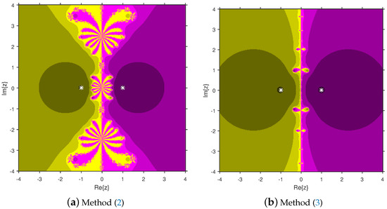
Figure 1. Comparison of attraction basins associated with second-degree polynomial $O_1\left(z\right)=z^2-1$.

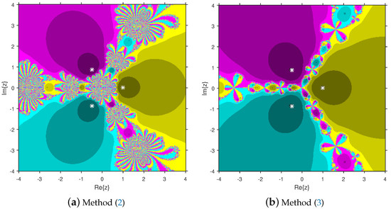
Figure 2. Comparison of attraction basins associated with third-degree polynomial $O_2\left(z\right)=z^3-1$.

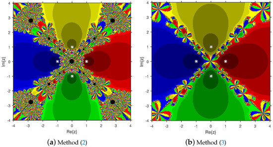
Figure 3. Comparison of attraction basins associated with fourth-degree polynomial $O_3\left(z\right)=z^4-1$.

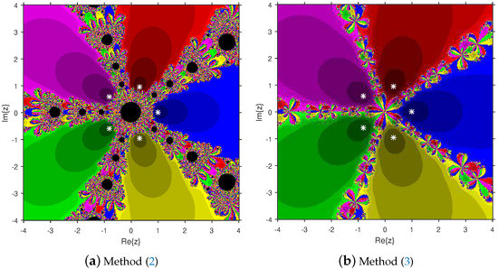
Figure 4. Comparison of attraction basins associated with fifth-degree polynomial $O_4\left(z\right)=z^5-1$.

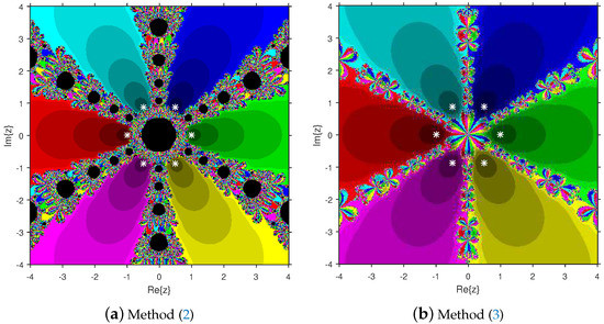
Figure 5. Comparison of attraction basins associated with sixth-degree polynomial $O_5\left(z\right)=z^6-1$.

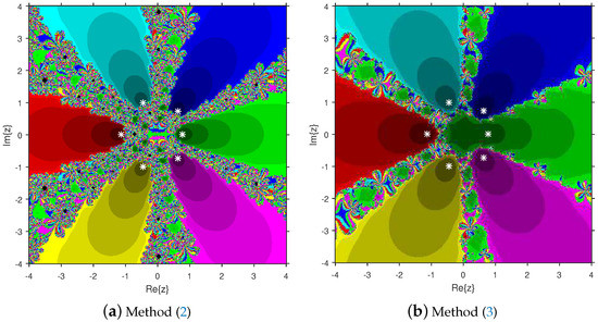
Figure 6. Comparison of attraction basins associated with sixth-degree polynomial $O_6\left(z\right)=z^6-z+1$.

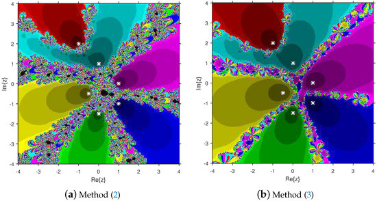
Figure 7. Comparison of attraction basins associated with sixth degree polynomial $O_7\left(z\right)=z^6-0.5z^5+\frac{11}{4}(1+i)z^4-\frac{1}{4}(19+3i)z^3+\frac{1}{4}(11+i)z^2-\frac{1}{4}(19+3i)z+\frac{3}{2}-3i$.

Based on the diagrams, we arrive at the conclusion that solver (12) has larger basins in comparison with solver (11). On the boundary points, solver (12) exhibits less chaotic behavior than (11). Moreover, the fractal pictures (Figure 3a, Figure 4a, Figure 5a, Figure 6a and Figure 7a) of formula (11) contain big black zones that demonstrate no convergence to the zeros of the corresponding polynomials. Therefore, we conclude that solver (12) is more numerically stable than solver (11). Hence, solver (12) is more preferable over solver (11) for practical use.

4. Numerical Examples

We apply the proposed techniques to estimate the convergence radii of iterative algorithms (2) and (3).

Example 1

([15]). Let $U_1=U_2={\mathbb{R}}^3$ and $V=\overline{S}(0,1)$. Consider D on V for $a={(a_1,a_2,a_3)}^t$ as

$$D\left(a\right)={(e^{a_1}-1,\frac{e-1}{2}{a}_2^2+a_2,a_3)}^t$$

We have $a_{\ast }={(0,0,0)}^t$. Then, $D^{\prime }\left(a_{\ast }\right)=I$, the identity operator. Let

$$D={(D_1,D_2,D_3)}^T,$$

where

$$D_1\left(h\right)=e^h-1,D_2\left(h\right)=\frac{e-1}{2}{h}^2+h,and{D}_3\left(h\right)=h.$$

In turn, we can write for $h_{\ast }=0$,

$$\begin{array}{cc}\hfill D_1^{\prime }\left(h\right)-D_1^{\prime }\left(h_{\ast }\right)& =e^h-1=h+\frac{h^2}{2!}+\cdots +\frac{h^n}{n!}+\cdots \hfill \\ \hfill & =\left(1+\frac{h}{2!}+\cdots +\frac{h^{n-1}}{n!}+\cdots \right)(h-h_{*}),\hfill \end{array}$$

So,

$$\begin{array}{cc}\hfill \parallel D_1^{\prime }{\left(h_{\ast }\right)}^{-1}(D_1^{\prime }\left(h\right)-D_1^{\prime }\left(h_{\ast }\right))\parallel & =|D_1^{\prime }{\left(h_{\ast }\right)}^{-1}(D_1^{\prime }\left(h\right)-D_1^{\prime }\left(h_{\ast }\right))|\hfill \\ \hfill & \le \left(1+\frac{1}{2!}+\cdots +\frac{1}{n!}+\cdots \right)|h-h_{\ast }|\hfill \\ \hfill & =(e-1)|h-h_{\ast }|,since|h|<1.\hfill \end{array}$$

Moreover, we have

$$|D_2^{\prime }{\left(h_{\ast }\right)}^{-1}(D_2^{\prime }\left(h\right)-D_2^{\prime }\left(h_{\ast }\right))|=|(e-1)h+1-I|=(e-1)|h-h_{\ast }|$$

and

$$|D_3^{\prime }{\left(h_{\ast }\right)}^{-1}(D_3^{\prime }\left(h\right)-D_3^{\prime }\left(h_{\ast }\right))|=0.$$

Hence, we can choose ${\Gamma }_0\left(h\right)=(e-1)h$. Then, the condition $\left(C_1\right)$ is validated. The equation ${\Gamma }_0\left(h\right)-1=0$ gives $(e-1)h-1=0$; so,

$$r_0=\frac{1}{e-1}and{V}_0=\overline{S}(0,1)\cap S\left(0,\frac{1}{e-1}\right)=S\left(0,\frac{1}{e-1}\right).$$

Concerning the third condition in $\left(C_2\right)$, recall that the divided difference is usually defined by

$$[b,h;D]=\frac{1}{2}(D^{\prime }\left(b\right)+D^{\prime }\left(h\right)),$$

or

$$[b,h;D]={\int }_0^1{D}^{\prime }(h+\theta (b-h))d\theta .$$

In either case, the left-hand side of the third condition gives

$$\begin{array}{cc}\hfill \parallel D^{\prime }{\left(h_{\ast }\right)}^{-1}([h,b;D]-D^{\prime }\left(h_{\ast }\right))\parallel & \le \frac{1}{2}\parallel D^{\prime }{\left(h_{\ast }\right)}^{-1}(D^{\prime }\left(h\right)-D^{\prime }\left(h_{\ast }\right))\parallel \hfill \\ \hfill & +\frac{1}{2}\parallel D^{\prime }{\left(h_{\ast }\right)}^{-1}(D^{\prime }\left(b\right)-D^{\prime }\left(h_{\ast }\right))\parallel .\hfill \end{array}$$

Therefore, we can choose

$${\Gamma }_2(h,s)=\frac{e-1}{2}(h+s).$$

Hence, by these choices of the functions $\Gamma ,{\Gamma }_1$ and ${\Gamma }_2$, the conditions $\left(C_2\right)$ are validated for this example. Similarly, for the first condition in $\left(C_2\right)$, notice that $D_1^{\prime }\left(h_{\ast }\right)=1$,

$$D_1^{\prime }\left(h_2\right)-D_1^{\prime }\left(h_1\right)=e^{h_2}-e^{h_1}=e^{h_3}(h_2-h_1)$$

for some $h_3$ between $h_1$ and $h_2$ with $|h_3|\le \frac{1}{e-1}$. It follows that

$$\parallel D^{\prime }{\left(h_{\ast }\right)}^{-1}(D^{\prime }\left(b\right)-D^{\prime }\left(h\right))\parallel \le e^{\frac{1}{e-1}}|b-h|.$$

Thus, the condition $\left(C_2\right)$ is verified for $\Gamma \left(h\right)=e^{\frac{1}{e-1}}h$. In order to validate the second condition in $\left(C_2\right)$, notice that

$$\begin{array}{cc}\hfill \parallel D^{\prime }{\left(h_{\ast }\right)}^{-1}{D}^{\prime }\left(h\right)\parallel & =\parallel D^{\prime }{\left(h_{\ast }\right)}^{-1}(D^{\prime }\left(h\right)-D^{\prime }\left(h_{\ast }\right)+D^{\prime }\left(h_{\ast }\right))\parallel \hfill \\ \hfill & \le \parallel D^{\prime }{\left(h_{\ast }\right)}^{-1}{D}^{\prime }\left(h_{\ast }\right)\parallel +\parallel D^{\prime }{\left(h_{\ast }\right)}^{-1}(D^{\prime }\left(h\right)-D^{\prime }\left(h_{\ast }\right))\parallel \hfill \\ \hfill & =1+{\Gamma }_0(\parallel h-h_{\ast }\parallel ).\hfill \end{array}$$

However, $1+{\Gamma }_0(\parallel h-h_{\ast }\parallel )\le 1+(e-1)\left|h\right|\le 2,$ since $\left|h\right|\le \frac{1}{e-1}$. Hence, if we choose ${\Gamma }_1\left(h\right)=2$, the second condition is $\left(C_2\right)$ is validated. Using proposed theorems, we obtain ρ and $\overline{\rho }$. These values are given in Table 1.

Table 1. Comparison of convergence radii for Example 1.

Method (2)	Method (3)
${\rho }_1=0.382692$	$\overline{{\rho }_1}=0.382692$
${\rho }_2=0.173524$	$\overline{{\rho }_2}=0.176270$
${\rho }_3=0.125226$	$\overline{{\rho }_3}=0.141600$
$\rho =0.125226$	$\overline{\rho }=0.141600$

Example 2

([1]). Let us consider $U_1=U_2=C[0,1]$ and $V=\overline{S}(0,1)$. Define D on V by

$$D\left(a\right)\left(v\right)=a\left(v\right)-5{\int }_0^{1}vya{\left(y\right)}^{3}dy,$$

where $a\left(v\right)\in C[0,1]$. It follows by this definition that the Fréchet derivative is given as

$$D^{\prime }\left(a\left[u\right]\right)\left(v\right)=u\left(v\right)-15{\int }_0^{1}Vya{\left(y\right)}^{2}u\left(y\right)dyforeachu\in V.$$

It follows by this definition that $D^{\prime }\left(a_{\ast }\right)=I$. If we substitute the last two formulas on the left-hand side of condition $\left(C_1\right)$ and use the max-norm on V, we see that

$$\parallel D^{\prime }{\left(a_{\ast }\right)}^{-1}(D^{\prime }\left(a\right)-D\left(a_{\ast }\right))\parallel \le {\Gamma }_0(\parallel a-a_{\ast }\parallel ),$$

provided that ${\Gamma }_0\left(h\right)=7.5h$; so, $r_0=\frac{1}{7.5}=\frac{2}{15}$ and $V_0=S\left(a_{\ast },\frac{2}{15}\right)$. Similarly, the first condition in $\left(C_2\right)$ gives

$$\parallel D^{\prime }{\left(a_{\ast }\right)}^{-1}(D^{\prime }\left(b\right)-D^{\prime }\left(a\right))\parallel \le \Gamma (\parallel b-a\parallel )$$

provided that $\Gamma \left(h\right)=15h$. Then, according to the work in Exercise 1, we can choose ${\Gamma }_1\left(h\right)=2$ and ${\Gamma }_2(h,s)=\frac{7.5}{2}(h+s)=\frac{15}{4}(h+s)$. The convergence radii ρ and $\overline{\rho }$ are obtained using the suggested theorems and presented in Table 2.

Table 2. Comparison of convergence radii for Example 2.

Method (2)	Method (3)
${\rho }_1=0.066667$	$\overline{{\rho }_1}=0.066667$
${\rho }_2=0.030318$	$\overline{{\rho }_2}=0.032019$
${\rho }_3=0.022658$	$\overline{{\rho }_3}=0.026150$
$\rho =0.022658$	$\overline{\rho }=0.026150$

Example 3

([16]). Let us consider $U_1=U_2=C[0,1]$ and $V=\overline{S}(0,1)$. Define the nonlinear integral equation as

$$D\left(a\right)\left(v\right)=a\left(v\right)-{\int }_0^{1}F(v,y)\frac{a{\left(y\right)}^2}{2}dy,$$

where $a\left(v\right)\in C[0,1]$ and $F(v,y)$ is given on $[0,1]\times [0,1]$ as

$$F(v,y)=\left\{\begin{array}{cc}(1-v)y,\hfill & \mathrm{if}y\le v\hfill \\ (1-y)v,\hfill & \mathrm{if}v\le y\hfill \end{array}.\right.$$

We have $a_{\ast }=0$. By repeating the work in Example 2 and using the max-norm, we see that $\parallel F\parallel \le \frac{1}{8}$. Therefore, we can choose ${\Gamma }_0\left(h\right)=\Gamma \left(h\right)=0.125h$, ${\Gamma }_1\left(h\right)=2$ and ${\Gamma }_2(h,s)=\frac{h+s}{16}$. We apply the suggested results to compute ρ and $\overline{\rho }$ (Table 3).

Table 3. Comparison of convergence radii for Example 3.

Method (2)	Method (3)
${\rho }_1=5.333333$	$\overline{{\rho }_1}=5.333333$
${\rho }_2=2.339380$	$\overline{{\rho }_2}=2.399363$
${\rho }_3=1.655689$	$\overline{{\rho }_3}=1.898871$
$\rho =1.655689$	$\overline{\rho }=1.898871$

5. Conclusions

The convergence balls as well as the dynamical behaviors of two efficient weighted-Newton-like equation solvers are compared. The ball convergence outcomes of methods (2) and (3) are produced by considering the generalized Lipschitz continuity of the first derivative only. Then, the complex dynamical behaviors of these algorithms are compared by employing the attraction basin tool. It is noticed that solver (3) has bigger basins than method (2). Lastly, our analytical findings are verified on application problems. It is found that method (3) has larger convergence balls than solver (2). Hence, solver (3) is better than method (2) for practical application. Our approach can be used to extend other methods [2,17,18,19,20] in a similar fashion. This will be the topic of our future research.

References

- Argyros, I.K. Unified Convergence Criteria for Iterative Banach Space Valued Methods with Applications. Mathematics 2021, 9, 1942. [Google Scholar] [CrossRef]
- Amat, S.; Busquier, S. Advances in Iterative Methods for Nonlinear Equations; Springer: Cham, Switzerland, 2016. [Google Scholar]
- Cordero, A.; Torregrosa, J.R. Variants of Newtons method using fifth-order quadrature formulas. Appl. Math. Comput. 2007, 190, 686–698. [Google Scholar]
- Potra, F. On Q-order and R-order of Convergence. J. Optim. Theory Appl. 1989, 63, 415–431. [Google Scholar] [CrossRef]
- Grau-Sánchez, M.; Gutiérrez, J.M. Zero-finder methods derived from Obreshkovs techniques. Appl. Math. Comput. 2009, 215, 2992–3001. [Google Scholar]
- Sharma, J.R.; Guna, R.K.; Sharma, R. An efficient fourth order weighted-Newton method for systems of nonlinear equations. Numer. Algor. 2013, 62, 307–323. [Google Scholar] [CrossRef]
- Cordero, A.; García-Maimó, J.; Torregrosa, J.R.; Vassileva, M.P. Solving nonlinear problems by Ostrowski-Chun type parametric families. J. Math. Chem. 2015, 53, 430–449. [Google Scholar] [CrossRef]
- Neta, B.; Scott, M.; Chun, C. Basins of attraction for several methods to find simple roots of nonlinear equations. Appl. Math. Comput. 2012, 218, 10548–10556. [Google Scholar]
- Petković, M.S.; Neta, B.; Petkovixcx, L.; Dzžunixcx, D. Multipoint Methods for Solving Nonlinear Equations; Elsevier: Amsterdam, The Netherlands, 2013. [Google Scholar]
- Sharma, J.R.; Arora, H. Improved Newton-like methods for solving systems of nonlinear equations. SeMA J. 2016, 74, 1–7. [Google Scholar] [CrossRef]
- Sharma, J.R.; Arora, H. On efficient weighted-Newton methods for solving systems of nonlinear equations. Appl. Math. Comput. 2013, 222, 497–506. [Google Scholar] [CrossRef]
- Grau-Sánchez, M.; Grau, Á.; Noguera, M. Ostrowski type methods for solving systems of nonlinear equations. Appl. Math. Comput. 2011, 218, 2377–2385. [Google Scholar] [CrossRef]
- Rheinboldt, W.C. An adaptive continuation process for solving systems of nonlinear equations. In Mathematical Models and Numerical Methods; Tikhonov, A.N., Ed.; Banach Center: Warsaw, Poland, 1978; pp. 129–142. [Google Scholar]
- Traub, J.F. Iterative Methods for Solution of Equations; Prentice-Hall: Upper Saddle River, NJ, USA, 1964. [Google Scholar]
- Argyros, I.K. The Theory and Applications of Iteration Methods, 2nd ed.; Engineering Series; CRC Press: Boca Raton, FL, USA; Taylor and Francis Group: Abingdon, UK, 2022. [Google Scholar]
- Argyros, I.K.; Magreñán, Á.A. A Contemporary Study of Iterative Methods; Elsevier: Amsterdam, The Netherlands; Academic Press: New York, NY, USA, 2018. [Google Scholar]
- Liu, T.; Qin, X.; Wang, P. Local Convergence of a Family of Iterative Methods with Sixth and Seventh Order Convergence under Weak Condition. Int. J. Comput. Methods 2019, 16, 1850120. [Google Scholar] [CrossRef]
- Scott, M.; Neta, B.; Chun, C. Basin attractors for various methods. Appl. Math. Comput. 2011, 218, 2584–2599. [Google Scholar] [CrossRef]
- Magreñán, Á.A. Different anomalies in a Jarratt family of iterative root-finding methods. Appl. Math. Comput. 2014, 233, 29–38. [Google Scholar]
- Hueso, J.L.; Martínez, E.; Torregrosa, J.R. Third and fourth order iterative methods free from second derivative for nonlinear systems. Appl. Math. Comput. 2009, 211, 190–197. [Google Scholar] [CrossRef]
Publisher’s Note: MDPI stays neutral with regard to jurisdictional claims in published maps and institutional affiliations. |
© 2022 by the authors. Licensee MDPI, Basel, Switzerland. This article is an open access article distributed under the terms and conditions of the Creative Commons Attribution (CC BY) license (https://creativecommons.org/licenses/by/4.0/).