Dynamics of Interacting Colloidal Particles Using the IIR Recursive Digital Filter Method

Abstract

This paper focuses on the numerical study of spherical particle sedimentation, taking into account hydrodynamic interactions. Infinite impulse response (IIR) digital filters, specially tailored to solve the sedimentation dynamics, were used in the present study to numerically solve the coupled ordinary differential equations with the time-dependent coefficients of the problem. Hydrodynamic interactions are modeled using the Rotne–Prager–Yamakawa (RPY) approximation, to which a correction is made to better account for short-range interactions. In order to validate both the proposed numerical resolution method and the RPY correction, this paper begins with the study of two interacting spherical particle sedimentation methods. Comparisons with previously published analytical or numerical results confirm the relevance of the present approach.

1. Introduction

The sedimentation of micro-particles (in the form of spheres, filaments, sheets, etc.) can represent a major obstacle to the effective use of colloidal suspensions in industrial environments. Colloidal particles experience gravitational, thermal, and hydrodynamic forces while moving in a fluid. The influence of the latter is a crucial aspect in various problems related to the mechanics and transport of suspensions. Important properties, such as the terminal sedimentation velocity of a suspension and the agglomeration rates of aerosols in the atmosphere, all depend on the relative motion of suspended particles [1]. The same applies to the effectiveness of spray purification devices (aimed at removing suspended particles from gas streams). In addition, knowledge of the velocity distribution of microparticles within a suspension is essential for example in granulometry, where it can be used to determine the size distribution of the considered particles.

From a particle point of view, colloidal suspensions are usually studied using the Stokesian dynamics (SD) method introduced by Brady and Bossis [2]. The SD method is based on solving the coupled Langevin equations describing the dynamics of N colloidal particles, which are written as follows when only translation is considered [2,3]:

$$m_i\frac{\mathrm{d}{\mathbf{v}}_i}{\mathrm{d}t}={\mathbf{F}}_i^h+{\mathbf{F}}_i^{nh}+{\mathbf{F}}_i^b,i=1,2,\cdots ,N$$

(1)

where $m_i$ and ${\mathbf{v}}_i$ are the mass and the velocity vector of the ith particle, respectively; ${\mathbf{F}}_i^h$ is the hydrodynamic force exerted by the fluid on the ith particle; ${\mathbf{F}}_i^{nh}$ are the non-hydrodynamic forces (interparticle forces ${\mathbf{F}}^{\mathrm{int}}$ and/or external forces ${\mathbf{F}}^e$) acting on the ith particle; and ${\mathbf{F}}_i^b$ is the Brownian force acting on the ith particle due to thermal agitation. The SD approach is implemented in well-known numerical codes such as Hoomd-Blues, Lammps, PyStokes, and many others. Langevin’s equations are generally solved in these codes using the over-damped assumption, which consists of neglecting the inertial terms $m_i\frac{\mathrm{d}{\mathbf{v}}_i}{\mathrm{d}t}$ in front of the viscous contribution to the hydrodynamic force ${\mathbf{F}}_i^h$, leading to the following simplified equation of motion:

$${\mathbf{F}}_i^h=-{\mathbf{F}}_i^{nh}-{\mathbf{F}}_i^b,i=1,2,\cdots ,N$$

(2)

In most unconstrained situations, the over-damped hypothesis yields remarkable results, provided that suspension behavior is only considered over long time scales, which is generally the case. However, when it comes to characterizing the local behavior of suspensions, i.e., at short times, the over-damped hypothesis may prove to be too imprecise. This is, for example, the case in optical two-point microrheology measurements [4,5]. It is therefore within the framework of a global dynamics study that the present modeling is carried out, by solving Equation (1) over the whole time-scale, using first-order infinite impulse response digital filters (IIR).

Infinite impulse response (IIR) digital filters are usually limited to the field of linear time-invariant systems (LTISs), of which their dynamics are described by linear ordinary differential equations with constant coefficients, or equivalently by Laplace transfer functions expressed as polynomial fractions. In a previous paper, the use of first-order IIR filters was extended to the numerical resolution of Basset-type integro-differential equations [6], of which their Laplace transfer functions cannot be expressed as rational fractions. A similar approach was adopted here in order to extend the IIR-Filter method to the numerical resolution of system (1), which is composed of N coupled ordinary differential equations (ODEs), satisfied based on the particle velocities: ${\mathbf{v}}_1$, ${\mathbf{v}}_2$, ⋯, and ${\mathbf{v}}_N$. These EDOs are linear as functions of velocities but non-linear as functions of particle positions ${\mathbf{r}}_1$, ${\mathbf{r}}_2$, ⋯, and ${\mathbf{r}}_N$. It is therefore an original extension of the IIR-Filter method that is proposed in the present paper.

This paper first examines the sedimentation dynamics of two identical spherical micro-particles to validate the method of solving the equations of the motion of colloidal particles in interactions using the IIR-Filter method. The results are compared with those obtained analytically or numerically, in other research works [7,8,9,10]. Stimson and Jeffery [7] delivered, for the first time, an exact solution of the axisymmetric translational motion for two spherical particles moving at the same speed along their centerline. The authors obtained the solution in the form of an infinite series, which converges rapidly using bipolar coordinates. This is not the case when the particles are very close to each other. The calculated values of the forces are for identical spheres. O’Neill [11] then Goldman et al. [8] and finally Wakiya [12] also used this technique. The authors aimed to determine the resulting motion of two identical, homogeneous-free spheres, moving in an unlimited fluid, with a low Reynolds number. They determined the linear and angular velocities of the two spheres as a function of their relative separation and the orientation of the line of centers concerning the direction of gravity $\mathbf{g}$.

Ganatos et al. [13] numerically solved the problem using the collocation technique. This technique was previously developed by other authors to process and study unbounded [14] and bounded [15] axisymmetric Stokes flows.

2. Resolution Method

Consider a finite number N of identical particles suspended in a base fluid with density ${\rho }_f$ and dynamic viscosity ${\mu }_f$ (see Figure 1). In this study, the fluid analyzed was assumed to be incompressible, Newtonian, unbounded, and at rest at significant distances from the colloidal particles. The particles themselves are assumed to be rigid, spherical, and have a radius of a. They are supposed to be small enough to make inertial forces negligible at long-time dynamics in comparison to viscosity forces, but large enough to make the effects of thermal agitation (Brownian motion) negligible. Fluid properties (density and viscosity) play a crucial role in the sedimentation processes, affecting the behavior of particles as they settle through a fluid medium. These properties are related to each other by the Reynolds number Re. In the whole study, viscous flow regimes with Re less than 1 were considered and, in the case of water, at room conditions (density ${\rho }_f={10}^3\mathrm{kg}/{\mathrm{m}}^3$ and shear viscosity ${\mu }_f=1\mathrm{mPa}·\mathrm{s}$). Suspended particles were assumed to be silica, with density ${\rho }_{\mathrm{PC}}=2\times {10}^3\mathrm{kg}/{\mathrm{m}}^3$ and radii of the order of a few micrometers, depending on the Reynolds numbers considered.

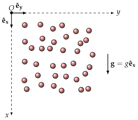
Figure 1. N spherical particles suspended in a viscous fluid initially at rest.

2.1. The Non-Hydrodynamic Forces

The dynamics of $N>1$ colloidal particles, including hydrodynamic interactions, were examined. The effect of thermal agitation was neglected, and only the translational motion was considered. The initial positions were chosen in such a way that the particles did not come into contact (no contact forces) and were not subjected to any surface tension forces (unbounded fluid). This was, therefore, the problem of the fall of N solid spheres into a viscous fluid at rest. The external forces ${\mathbf{F}}_i^e$ (other than hydrodynamic) considered here were the weight ${\mathbf{P}}_i$ and the Archimedes thrust ${\Pi }_i$, which were exerted on particle $\left(i\right)$:

$${\mathbf{F}}_i^e={\mathbf{P}}_i+{\Pi }_i=m_i\left(1-{\rho }_f/{\rho }_{\mathrm{PC}}\right)g{\widehat{\mathbf{e}}}_x$$

(3)

where ${\rho }_{\mathrm{PC}}$ is the colloidal particle (PC) density. In addition, the non-hydrodynamic forces ${\mathbf{F}}_i^{nh}$ may also contain contact forces ${\mathbf{F}}_{ij}^c$ (of the Hertz–Voigt type for example), which was not taken into account in the present study.

2.2. The Hydrodynamic Interactions

Hydrodynamic interactions (HIs) are transmitted by the fluid between the particles that move through it. These interactions explain various observed effects. It is, for example, possible to understand the tendency of small objects to fall vertically or at different speeds if close enough during sedimentation. The hydrodynamic interactions ${\mathbf{F}}_i^h$ originate from the movement of the solvent (host liquid), which is described by the Stokes equation and is influenced locally and at a distance by the motion of the PCs. These disturbances are then transmitted by the solvent to the other PCs that compose the suspension, modifying its trajectories. These interactions are particularly significant in the case of concentrated suspensions, where the $\varphi$ solid volume fraction is high. The disturbances caused by the fluid flow are assumed to be rapid enough (at the scale of colloidal particles) in comparison to the movement of the PCs. This means that flow induced disturbances propagation can, to a good approximation, be considered almost instantaneous [16].

Under these conditions, the flow of the fluid at a given time t is only a function of the positions and velocities of the N PCs that compose the suspension. Thus, the hydrodynamic force ${\mathbf{F}}_i^h$ exerted by the solvent on the PC $\left(i\right)$ is a function of the N position vectors ${\mathbf{r}}_j$ and the N velocity vectors ${\mathbf{v}}_j$ of the PCs:

$${\mathbf{F}}_i^h={\mathbf{F}}_i^h\left({\mathbf{r}}_1,\cdots ,{\mathbf{r}}_N;{\mathbf{v}}_1,\cdots ,{\mathbf{v}}_N\right)$$

(4)

The linearity of the Stokes equation allows us to establish the relationships between the translational velocities of particles and the forces acting on them. The hydrodynamic interactions between colloidal particles are expressed using the mobility tensor and the associated mobility matrix $\left({\mathcal{M}}^{\mathrm{d},\mathrm{d}}\right)$. The components ${\mathcal{M}}_{ij}^{\mathrm{d},\mathrm{d}}$ can be computed using a variety of methods [17,18]. The following relation defines the coefficients of the mobility matrix in the case of pure translation and a uniform imposed bulk flow ${\mathbf{v}}^{\infty }$:

$${\mathbf{v}}_i-{\mathbf{v}}^{\infty }=-\sum _{j=1}^N{\mathcal{M}}_{ij}^{\mathrm{d},\mathrm{d}}\left({\mathbf{r}}_1,\cdots ,{\mathbf{r}}_N\right)·{\mathbf{F}}_j^h$$

(5)

The mobilitymatrix $\left({\mathcal{M}}^{\mathrm{d},\mathrm{d}}\right)$ is a symmetrical square matrix $d\times d$, with d being the dimensionality of the suspension (i.e., $d=3$ here). There is no general analytic expression of the mobility matrix $\left({\mathcal{M}}^{\mathrm{d},\mathrm{d}}\right)$ for $N>2$. However, the expression of the matrix $\left({\mathcal{M}}^{\mathrm{d},\mathrm{d}}\right)$ can be simplified when only binary interactions are considered. Equation (5) is then written in the following simplified form, which will be systematically used in this work:

$${\mathbf{v}}_i-{\mathbf{v}}^{\infty }=-\sum _{j=1}^{j=N}{\mathcal{M}}_{ij}^{\mathrm{d},\mathrm{d}}\left({\mathbf{r}}_i,{\mathbf{r}}_j\right)·{\mathbf{F}}_j^h$$

(6)

where the flow velocity ${\mathbf{v}}^{\infty }$ of the fluid in the absence of particles is assumed to be zero throughout this study (fluid initially at rest). In assuming that the suspension has spherical symmetry, the ${\mathcal{M}}_{ij}^{\mathrm{d},\mathrm{d}}\left({\mathbf{r}}_i,{\mathbf{r}}_j\right)$ coefficients can be written as ${\mathcal{M}}_{ij}^{\mathrm{d},\mathrm{d}}\left(r_{ij}\right)$ with $r_{ij}=\parallel {\mathbf{r}}_i-{\mathbf{r}}_j\parallel$. The hydrodynamic forces ${\mathbf{F}}_j^h$ can then be determined by reversing the relation (6), i.e., by calculating the matrix ${\left({\mathcal{M}}^{\mathrm{d},\mathrm{d}}\right)}^{-1}$.

2.3. Expressions of the Mobility Matrix Coefficients

The main purpose of this section is to define the approximate expressions of the mobility matrix coefficients. Two common approximations are presented: the quasi-point approximation (AQP) and the Rotne–Prager–Yamakawa approximation (RPY).

2.3.1. The Quasi-Point Approximation (QPA)

In the quasi-point approximation, which is the most rudimentary approach, each sphere is assimilated to a source point, also called a Stokeslet. The so-called reflection method makes it possible to iteratively take into account hydrodynamic interactions. To analyze the hydrodynamic interactions between two spheres of radii $a_1$ and $a_2$, we can limit ourselves to the first reflection between two PCs, (1) and (2), and apply Faxen’s laws [19]. This helps us write the mobility matrix in the form of (7), which takes into account the Oseen–Burgers tensor $\overline{\overline{S}}$. For two spheres in three dimensions, this equation can be expressed as follows:

$$\left|\begin{array}{cc}\hfill {}_{\mathrm{AQP}}\mathcal{M}_{11}& =\frac{{\mathbb{I}}_3}{6\pi {\mu }_f{a}_1}\hfill \\ \hfill {}_{\mathrm{AQP}}\mathcal{M}_{22}& =\frac{{\mathbb{I}}_3}{6\pi {\mu }_f{a}_2}\hfill \\ \hfill {}_{\mathrm{AQP}}\mathcal{M}_{12}& {=}_{\mathrm{AQP}}{\mathcal{M}}_{21}=\frac{{\overline{\overline{S}}}_{12}}{8\pi {\mu }_f}=\frac{1}{8\pi {\mu }_f}\left(\frac{{\mathbb{I}}_3}{r_{12}}+\frac{{\mathbf{r}}_{\mathbf{12}}·{\mathbf{r}}_{\mathbf{12}}}{r_{12}^3}\right)\hfill \end{array}\right.$$

(7)

where ${\mathbb{I}}_3$ is the identity matrix (for $d=3$) and $r_{12}=\parallel {\mathbf{x}}_{\mathbf{1}}-{\mathbf{x}}_{\mathbf{2}}\parallel$. We recall here that ${\mathbf{r}}_{12}·{\mathbf{r}}_{12}$ is not a scalar but a tensor, with components that are given in Cartesian coordinates by

$${\mathbf{r}}_{12}·{\mathbf{r}}_{12}=\left(\begin{array}{ccc}{(x_1-x_2)}^2& (x_1-x_2)(y_1-y_2)& (x_1-x_2)(z_1-z_2)\\ (x_1-x_2)(y_1-y_2)& {(y_1-y_2)}^2& (y_1-y_2)(z_1-z_2)\\ (x_1-x_2)(z_1-z_2)& (y_1-y_2)(z_1-z_2)& {(z_1-z_2)}^2\end{array}\right)$$

(8)

As an illustration, the translational mobility matrix is expressed here for two identical spheres and $d=3$:

$$\left({}_{\mathrm{AQP}}\mathcal{M}\right)=\frac{1}{8\pi {\mu }_f{r}_{12}^3}\left(\begin{array}{cc}\frac{4r_{12}^3}{3a}{\mathbb{I}}_3& r_{12}^2{\mathbb{I}}_3+{\mathbf{r}}_{12}·{\mathbf{r}}_{12}\\ r_{12}^2{\mathbb{I}}_3+{\mathbf{r}}_{12}·{\mathbf{r}}_{12}& \frac{4r_{12}^3}{3a}{\mathbb{I}}_3\end{array}\right)$$

(9)

where ${\mathbf{r}}_{12}·{\mathbf{r}}_{12}$ is given by (8). Even if an analytic inversion of this $2d\times 2d$ matrix is possible, it leads to humanly unusable expressions. Numerical inversion is therefore preferable for determining hydrodynamic forces ${\mathbf{F}}_i^h$.

2.3.2. Rotne–Prager–Yamakawa (RPY) Approximation

This approximation is more accurate than the quasi-point approximation developed earlier. In the present study, the expression of the Rotne–Prager–Yamakawa tensor (RPY) proposed by Wajnryb et al. [20,21] is used for two different spheres of radii $a_1$ and $a_2$ in the absence of penetration ($r_{12}>a_1+a_2$). The matrix representation of mobility for two different spheres is given in this case by

$$\left|\begin{array}{cc}\hfill {}_{\mathrm{RPY}}\mathcal{M}_{11}& =\frac{{\mathbb{I}}_3}{6\pi {\mu }_f{a}_1}\hfill \\ \hfill {}_{\mathrm{RPY}}\mathcal{M}_{22}& =\frac{{\mathbb{I}}_3}{6\pi {\mu }_f{a}_2}\hfill \\ \hfill {}_{\mathrm{RPY}}\mathcal{M}_{12}& {=}_{\mathrm{RPY}}{\mathcal{M}}_{21}=\frac{1}{8\pi {\mu }_f{r}_{12}}\left[\left(1+\frac{a_1^2+a_2^2}{3r_{12}^2}\right){\mathbb{I}}_3+\left(1-\frac{a_1^2+a_2^2}{r_{12}^2}\right)\frac{{\mathbf{r}}_{\mathbf{12}}·{\mathbf{r}}_{\mathbf{12}}}{r_{12}^2}\right]\hfill \end{array}\right.$$

(10)

Let us recall the main properties of this approximation:

• At the limit where $r_{12}\gg sup(a_1,a_2)$, the Rotne–Prager–Yamakawa mobility matrix tends to be the mobility matrix of the point approximation. This turns out to be legitimate and corresponds to the so-called far-field hypothesis.
• When both spheres have the same radius, the following expression for the generalized mobility matrix is obtained:

  $$\left|\begin{array}{cc}\hfill {}_{\mathrm{RPY}}\mathcal{M}_{11}& {=}_{\mathrm{RPY}}{\mathcal{M}}_{22}=\frac{{\mathbb{I}}_3}{6\pi {\mu }_{f}a}\hfill \\ \hfill {}_{\mathrm{RPY}}\mathcal{M}_{12}& {=}_{\mathrm{RPY}}{\mathcal{M}}_{21}=\frac{1}{8\pi {\mu }_f{r}_{12}}\left[\left(1+\frac{2a^2}{3r_{12}^2}\right){\mathbb{I}}_3+\left(1-\frac{2a^2}{r_{12}^2}\right)\frac{{\mathbf{r}}_{\mathbf{12}}·{\mathbf{r}}_{\mathbf{12}}}{r_{12}^2}\right]\hfill \end{array}\right.$$

  (11)

The literatureevaluates the coefficients of the mobility matrix for different configurations. Kim et al. [22] performed the computation of coefficients for two identical spheres, while Jeffrey and Onishi [23] considered two different spheres, using the Lamb expression [24]. Perkins and Jones [25] were interested in the case of a single particle close to a flat wall, while Beenakker et al. [26] examined the case of several particles in the presence of a wall. Finally, Van Saarloos and Mazur [27] studied the case of several particles suspended in an infinite fluid.

2.4. Equations of Motion

The centers of inertia $C_j$ of spherical particles are assumed to be initially located in the $z=0$ plane. The initial position of $C_j$ is supposed to be ${\mathbf{OC}}_{\mathbf{i}}\left(0\right)=(x_i^0,y_i^0,0)$.

In applying Newton’s second law to each particle, the resulting system of coupled ordinary differential equations is as follows:

$$\left(\begin{array}{c}{m}_1{\dot{\mathbf{v}}}_1\\ :\\ m_i{\dot{\mathbf{v}}}_i\\ :\\ m_N{\dot{\mathbf{v}}}_N\end{array}\right)+{\left({\mathcal{M}}^{\mathrm{d},\mathrm{d}}\right)}^{-1}·\left(\begin{array}{c}{\mathbf{v}}_1\\ :\\ {\mathbf{v}}_i\\ :\\ {\mathbf{v}}_N\end{array}\right)=\left(\begin{array}{c}{\mathbf{P}}_1+{\Pi }_1\\ :\\ {\mathbf{P}}_i+{\Pi }_i\\ :\\ {\mathbf{P}}_N+{\Pi }_N\end{array}\right)$$

(12)

where ${\left({\mathcal{M}}^{\mathrm{d},\mathrm{d}}\right)}^{-1}$ is the inverse of the mobility matrix defined above.

The present study sought to solve system (12) with zero initial conditions on the velocities: ${\mathbf{v}}_{\mathbf{i}}\left(0\right)=\mathbf{0},\forall i=1,2,\cdots ,N$. System (12) is rewritten as follows:

$${\dot{\mathbf{v}}}_i\left(t\right)+{\alpha }_i\sum _{j=1}^{j=N}\left({\mathcal{M}}_{ij}^{-1}\right)·{\mathbf{v}}_j\left(t\right)={\alpha }_i{\mathbf{F}}_i^e\left(t\right)$$

(13)

where ${\alpha }_i=1/m_i$, and $\left({\mathcal{M}}_{ij}^{-1}\right)$ is a $d\times d$ matrix, with coefficients given by (7) or (10), depending on the considered approximation. To our knowledge, there is no systematic exact analytic approach (such as a Laplace transformation or variation of the constant) for solving the system analytically (13). Thus, the resolution exposed in the present study is based on a numerical approach that implements recursive IIR digital filters (the IIR-Filter method). This type of numerical approach has been successfully used to solve linear parabolic partial differential equations from heat conduction problems [28,29]. It has also been used to solve linear convolutional integro-differential equations in fluid mechanics [6]. In the former case, the time complexity of the IIR-Filter method is $O\left(n\right)$, which is lower than numerical methods such as a piecewise linear approximation, which features a time complexity of $O\left(n^2\right)$.

The present study extends the scope of the IIR-Filter method to the case of systems of linearly coupled ordinary differential equations with time-dependent coefficients.

2.5. Numerical Resolution Using the IIR-Filter Method

Let us first write ${\mathrm{NI}}_i\left({\mathbf{v}}_{\mathbf{1}},{\mathbf{v}}_{\mathbf{2}},\cdots ,{\mathbf{v}}_{\mathbf{N}}\right)={\sum }_{j=1}^N\left({\mathcal{M}}_{ij}^{-1}\right)·{\mathbf{v}}_j\left(t\right)$ as the non-time-invariant term in the system of Equation (13) for particle $\left(i\right)$. The mobility matrix depends on the positions of the particles that are in motion. Therefore, these positions change continuously over time, and the components of the mobility tensor also vary over time. This represents a considerable difficulty for the numerical solution of the equations of motion. The application of the Laplace transform $\mathcal{L}$ to system (13) leads to the following system of algebraic equations:

$$s{\overline{\mathbf{v}}}_i\left(s\right)-{\mathbf{v}}_i\left(0\right)={\alpha }_i{\overline{\mathbf{F}}}_i^e\left(s\right)-{\alpha }_i{\overline{\mathrm{NI}}}_i\left(s\right)$$

(14)

where ${\overline{\mathbf{v}}}_i\left(s\right)$, ${\overline{\mathbf{F}}}_i^e\left(s\right)$, and ${\overline{\mathrm{NI}}}_i\left(s\right)$ are the Laplace transforms of ${\mathbf{v}}_i$, ${\mathbf{F}}_i^e$, and ${\mathrm{NI}}_i$, respectively. Since there is no known analytic expression of velocities ${\mathbf{v}}_i$ that verifies (13), the Laplace transform ${\overline{\mathrm{NI}}}_i\left(s\right)$ of the non-invariant term ${\mathrm{NI}}_i$ cannot be computed analytically. Any direct analytic or numerical inversion of ${\overline{\mathbf{v}}}_i\left(s\right)$ (i.e., using an analytic expression of ${\overline{\mathbf{v}}}_i\left(s\right)$), thus becomes impossible. In this case, the numerical resolution must use methods that do not require knowledge of ${\overline{\mathrm{NI}}}_i\left(s\right)$. The IIR-Filter method allows for this. This is the main interest of the digital approach developed in this work. We recall that, for simplicity, this study is based on the assumption that ${\mathbf{v}}_i\left(0\right)=\mathbf{0}$. In the framework of the IIR-Filter method, the excitatory force ${\mathbf{F}}_i^e\left(t\right)$ must be sampled into a regular set of discrete values in time $\left\{{\mathbf{F}}_i^e\left(n{T}_e\right)\right\}$, where $T_e=\Delta t$ is the sampling period, in order to calculate the velocity ${\mathbf{v}}_i\left(n{T}_e\right)$.

The application to Equation (14) of the bilinear transformation of the type $s\to \frac{2}{T_e}\frac{z-1}{z+1}$ [30], allows the transition from Laplace space to discrete time space, with z being the complex number introduced in the definition of the z-transformation ($\mathcal{Z}$) of a discrete time signal $x\left(n{T}_e\right)$: $\mathcal{Z}\left[x\left(n{T}_e\right)\right]=\overline{x}\left(z\right)={\sum }_{n=0}^{\infty }x\left(n{T}_e\right)z^{-n}$.

Replacing s with $\frac{2}{T_e}\frac{z-1}{z+1}=\frac{2}{T_e}\frac{1-z^{-1}}{1+z^{-1}}$ in Equation (14) yields

$$\left(\frac{1-z^{-1}}{1+z^{-1}}\right){\overline{\mathbf{v}}}_i\left(z\right)=\frac{{\alpha }_i{T}_e}{2}\left({\overline{\mathbf{F}}}_i^e\left(z\right)-{\overline{\mathrm{NI}}}_i\left(z\right)\right)$$

resulting in the following algebraic system, with the intervention of the z-transforms of the different functions of the problem:

$$\left(1-z^{-1}\right){\overline{\mathbf{v}}}_i\left(z\right)=\frac{{\alpha }_i{T}_e}{2}\left(1+z^{-1}\right)\left({\overline{\mathbf{F}}}_i^e\left(z\right)-{\overline{\mathrm{NI}}}_i\left(z\right)\right)$$

(15)

In noting that the non-invariant term ${\mathrm{NI}}_i\left({\mathbf{v}}_{\mathbf{1}},{\mathbf{v}}_{\mathbf{2}},\cdots ,{\mathbf{v}}_{\mathbf{N}}\right)={\sum }_{j=1}^N\left({\mathcal{M}}_{ij}^{-1}\right)·{\mathbf{v}}_j\left(t\right)$ can be written as

$${\mathrm{NI}}_i\left(t\right)=\left({\mathcal{M}}_{ii}^{-1}\right)·{\mathbf{v}}_i\left(t\right)+\sum _{\begin{array}{c}j=1\\ j\ne i\end{array}}^N\left({\mathcal{M}}_{ij}^{-1}\right)·{\mathbf{v}}_j\left(t\right),$$

(16)

system (15) is rewritten in the following form:

$$\begin{array}{cc}\hfill \mathcal{Z}\left[\left({\mathbb{I}}_3+\frac{{\alpha }_i{T}_e}{2}\left({\mathcal{M}}_{ii}^{-1}\right)\right)·{\mathbf{v}}_i\right]& =z^{-1}\mathcal{Z}\left[\left({\mathbb{I}}_3-\frac{{\alpha }_i{T}_e}{2}\left({\mathcal{M}}_{ii}^{-1}\right)\right)·{\mathbf{v}}_i\right]+\frac{{\alpha }_i{T}_e}{2}\left(1+z^{-1}\right){\overline{\mathbf{F}}}_i^e\left(z\right)\hfill \\ \hfill & -\frac{{\alpha }_i{T}_e}{2}{\displaystyle \sum _{\begin{array}{c}j=1\\ j\ne i\end{array}}^N}\left\{\mathcal{Z}\left[\left({\mathcal{M}}_{ij}^{-1}\right)·{\mathbf{v}}_j\right]+z^{-1}\mathcal{Z}\left[\left({\mathcal{M}}_{ij}^{-1}\right)·{\mathbf{v}}_j\right]\right\}\hfill \end{array}$$

(17)

From these algebraic z-equations, N coupled recurrence relations are deduced to numerically solve the problem of the dynamics of N spherical colloidal particles at time $t_n=n{T}_e$, taking into account hydrodynamic interactions:

$$\begin{array}{cc}\hfill {\left[{\mathbb{I}}_3+\frac{{\alpha }_i{T}_e}{2}\left({\mathcal{M}}_{ii}^{-1}\right)\right]}_n·{\mathbf{v}}_{i,n}& ={\left[{\mathbb{I}}_3-\frac{{\alpha }_i{T}_e}{2}\left({\mathcal{M}}_{ii}^{-1}\right)\right]}_{n-1}·{\mathbf{v}}_{i,n-1}+\frac{{\alpha }_i{T}_e}{2}\left({\mathbf{F}}_{i,n}^e+{\mathbf{F}}_{i,n-1}^e\right)\hfill \\ \hfill & -\frac{{\alpha }_i{T}_e}{2}{\displaystyle \sum _{\begin{array}{c}j=1\\ j\ne i\end{array}}^N}\left[{\left({\mathcal{M}}_{ij}^{-1}\right)}_n·{\mathbf{v}}_{j,n}+{\left({\mathcal{M}}_{ij}^{-1}\right)}_{n-1}·{\mathbf{v}}_{j,n-1}\right]\hfill \end{array}$$

(18)

where $n=1,2,\cdots ,N$, and ${\mathbf{r}}_{i,n}={\mathbf{r}}_{i,n-1}+T_e{\mathbf{v}}_{i,n-1}$.

Key result (18) is applied, in the following paragraphs, to the calculation of the dynamics of systems composed of two, and then three, colloidal particles, when hydrodynamic interactions are not negligible. The flowchart shown in Figure A1 summarizes the process of numerically solving the coupled recursion Equations (18) of the Stokesian dynamics of a colloidal suspension using the IIR-Filter method.

2.6. Full Dynamics versus Long-Time Dynamics

To test the relevance of numerically solving Equation (1) rather than (2), we consider here an elementary system in which two identical particles drive through hydrodynamic interactions, a third particle initially at rest (see Figure 2). The equations of motion are, in this case, neglecting the influences of gravity and thermal agitation:

$$\left|\begin{array}{cc}\hfill m_1{\dot{\mathbf{U}}}_1& ={\mathbf{F}}_1^h\left({\mathbf{r}}_1,{\mathbf{r}}_2,{\mathbf{r}}_3;{\mathbf{U}}_1,{\mathbf{U}}_2,{\mathbf{U}}_3\right)\hfill \\ \hfill \mathbf{0}& ={\mathbf{F}}_2^h\left({\mathbf{r}}_1,{\mathbf{r}}_2,{\mathbf{r}}_3;{\mathbf{U}}_1,{\mathbf{U}}_2,{\mathbf{U}}_3\right)+{\mathbf{F}}_2^e\hfill \\ \hfill \mathbf{0}& ={\mathbf{F}}_3^h\left({\mathbf{r}}_1,{\mathbf{r}}_2,{\mathbf{r}}_3;{\mathbf{U}}_1,{\mathbf{U}}_2,{\mathbf{U}}_3\right)+{\mathbf{F}}_3^e\hfill \end{array}\right.$$

(19)

where ${\mathbf{F}}_2^e$ and ${\mathbf{F}}_3^e$ are the external forces that must be exerted on ${\mathcal{C}}_2$ and ${\mathcal{C}}_3$, respectively, in order for them to move with uniform rectilinear translational motion.

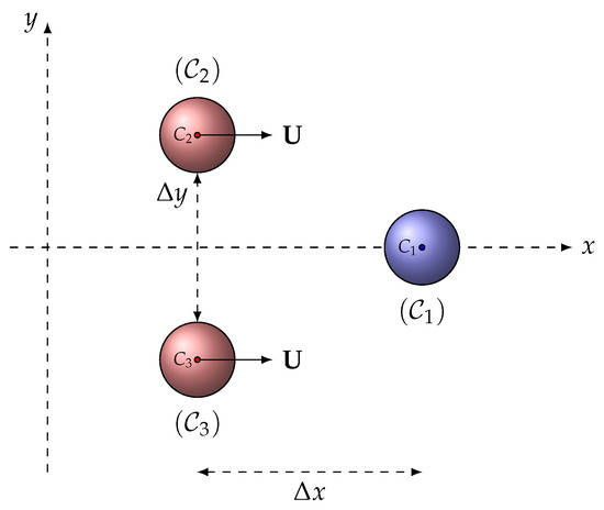
Figure 2. Two identical particles (${\mathcal{C}}_2$ and ${\mathcal{C}}_3$), moving according to a uniform rectilinear translation at the same velocity ${\mathbf{U}}_{\mathbf{2}}={\mathbf{U}}_{\mathbf{3}}=\mathbf{U}=U{\mathbf{e}}_x$, are driven by hydrodynamic interactions to a third particle (${\mathcal{C}}_1$), initially at rest.

The dynamics, Equation (19), are solved using the IIR-Filter method (full dynamics) and also using the usual over-damped assumption (long-time dynamics).

We considered the case of three identical spherical particles (radius $a=10\mathsf{\mu }\mathrm{m}$) made of silica (density ${\rho }_{\mathrm{PC}}=2\times {10}^3\mathrm{kg}/{\mathrm{m}}^3$), immersed in water at rest, at room conditions (dynamic viscosity ${\mu }_f=1\mathrm{mPa}·\mathrm{s}$ and density ${\rho }_f={10}^3\mathrm{kg}/{\mathrm{m}}^3$). ${\mathcal{C}}_2$ and ${\mathcal{C}}_3$ are assumed to move at constant velocity $\mathbf{U}=U{\mathbf{e}}_x$, with $U=10\mathrm{cm}/\mathrm{s}$, and it is assumed that, initially, $\Delta y=100\mathsf{\mu }\mathrm{m}$ and $\Delta x=10a$. Equation (19) has been solved with a time step $T_e=2\mathsf{\mu }\mathrm{s}$.

Figure 3a compares the short-time dynamics of ${\mathcal{C}}_1$, obtained without over-damping (solid line) and with over-damping (dotted line). It is clear from this figure that short-time dynamics are not well described in the present situation by the over-damped approximation. It is also clear from Figure A2 that the two approaches converge at the long-time scale of observation.

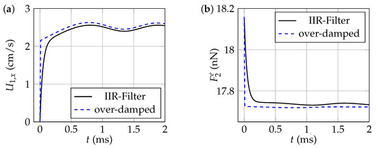
Figure 3. Comparisons of ${\mathcal{C}}_1$ short-time dynamics, obtained without making the over-damped assumption (solid line) and making the over-damped assumption (dashed line). (a) Changes in the $U_{1,x}$ component of ${\mathcal{C}}_1$’s velocity as a function of time. (b) Changes in the external force ${\mathbf{F}}_2^e$ exerted on ${\mathcal{C}}_2$, as a function of time.

In the same way, Figure 3b shows that the external force ${\mathbf{F}}_2^e$ required to ensure uniform rectilinear motion of ${\mathcal{C}}_2$ (or ${\mathcal{C}}_3$) is not precisely calculated for short time scales using the over-damped method.

It can be concluded from this elementary study that measurements based on long-time results can easily be obtained by the over-damped method and possibly also by the IIR-Filter method (which is undoubtedly more complex to implement). If, on the other hand, it is necessary to evaluate the dynamics of colloidal particles at short time scales, it is imperative in this case to resort to solving the equations of motion without making the over-damped approximation. In this case, the IIR-Filter method is an interesting approach, as illustrated in the following paragraphs.

3. Sedimentation of Two Identical Colloidal Particles

The configuration of two identical spherical particles is a simple and effective way to test the accuracy and convergence of the numerical resolution method presented in the present study (result (18)). The numerical results obtained using our approach are first compared with approximate or numerical analytical solutions available in the literature. The “ideal” configuration, where two identical spherical particles sedimenting at small Reynolds numbers in a viscous fluid at rest and unbounded, has numerous applications in colloid chemistry, rheology, meteorology, and the sedimentation of dilute suspensions.

3.1. Presentation

Let us consider the sedimentation problem of two identical spherical particles of radius a, density ${\rho }_{\mathrm{PC}}$, and suspended without initial velocity (${\mathbf{v}}_1\left(0\right)=\mathbf{0}$ and ${\mathbf{v}}_2\left(0\right)=\mathbf{0}$) in a solvent initially at rest (${\mathbf{v}}^{\infty }=\mathbf{0}$), with viscosity ${\mu }_f$ and density ${\rho }_f$ (see Figure 4).

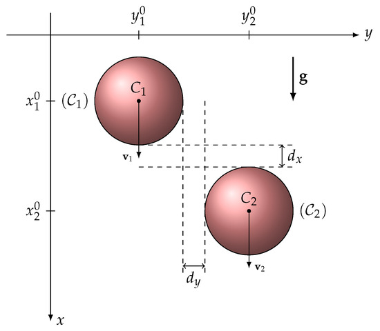
Figure 4. Sedimentation of two identical spheres in a stationary fluid.

The centers of inertia $C_1$ and $C_2$ of the two spherical particles are placed in the $z=0$ plane. The initial positions of $C_1$ and $C_2$ are ${\mathbf{OC}}_{\mathbf{1}}\left(0\right)=(x_1^0,y_1^0,0)$ and ${\mathbf{OC}}_{\mathbf{2}}\left(0\right)=(x_2^0,y_2^0,0)$. We need to solve the system of coupled differentials, Equation (12), which becomes, in the case of $N=2$, identical to the following particles:

$$m\left(\begin{array}{c}{\dot{\mathbf{v}}}_1\\ {\dot{\mathbf{v}}}_2\end{array}\right)+{\left({\mathcal{M}}^{d,d}\right)}^{-1}·\left(\begin{array}{c}{\mathbf{v}}_1\\ {\mathbf{v}}_2\end{array}\right)=\left(\begin{array}{c}{\mathbf{P}}_1+{\Pi }_1\\ {\mathbf{P}}_2+{\Pi }_2\end{array}\right)$$

(20)

with the initial conditions ${\mathbf{v}}_{\mathbf{1}}\left(0\right)=\mathbf{0}$ and ${\mathbf{v}}_{\mathbf{2}}\left(0\right)=\mathbf{0}$. By explaining the various vectors, we obtain here

$$m\left(\begin{array}{c}{\dot{v}}_{1x}\\ {\dot{v}}_{1y}\\ {\dot{v}}_{1z}\\ {\dot{v}}_{2x}\\ {\dot{v}}_{2y}\\ {\dot{v}}_{2z}\end{array}\right)=-{\left({\mathcal{M}}^{d,d}\left(r_{12}\right)\right)}^{-1}·\left(\begin{array}{c}{v}_{1x}\\ v_{1y}\\ v_{1z}\\ v_{2x}\\ v_{2y}\\ v_{2z}\end{array}\right)+mg\left(1-\frac{{\rho }_f}{{\rho }_{\mathrm{PC}}}\right)\left(\begin{array}{c}1\\ 0\\ 0\\ 1\\ 0\\ 0\end{array}\right)$$

(21)

3.2. The Results

Equation (21), describing the fall dynamics of two identical spheres, is solved using recurrence relations (18). One of our objectives was to choose among the two approximations mentioned above the one that delivers the results closest to physical reality. The two spheres are initially placed at the same altitude $x_1^0=x_2^0$, with the centers being $2a_1+\mathrm{d}y$ apart. When the two particles settle, they remain at the same distance from each other by moving at the same speed, denoted $v_x$. This is a consequence of the reversibility property of flows at low Reynolds numbers. This common velocity of the two particles is higher than the velocity that each of them would have taken separately. The smaller the initial distance between the particles, the greater the speed of the doublet.

Figure 5a shows the temporal variations in the $v_x$ component of the two particles. Figure 5b compares the limit velocity of the fall of a single sphere $V_s^0=\frac{mg}{6\pi {\mu }_{f}a}\left(1-\frac{{\rho }_f}{{\rho }_{\mathrm{PC}}}\right)$ with $v_x^{\ell ,\mathrm{HI}}$ obtained numerically in the presence of a second identical sphere, for the initial conditions indicated above. The verticality of the fall is checked ($v_{1y}=v_{2y}=0$ m/s) as well as its location in the $z=0$ plane.

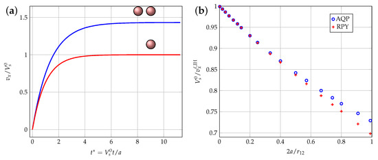
Figure 5. Fall velocities of two identical spheres taking into account hydrodynamic interactions. (a) Changes in the $v_x$ component of the two spheres as a function of reduced time $t^{*}$. (b) Changes in the fall velocity $v_x^{\ell ,\mathrm{HI}}$ of the two spheres relative to the limit fall velocity $V_s^0$ of one sphere, as a function of $2a/r_{12}$.

Figure 5b legitimately reveals that both the RPY and AQP approximations tend toward a common limit when the distance $r_{12}$ between the centers of the two spheres becomes large in front of their diameter $d=2a$. The physical reason for this common limit lies in the fact that at a high distance from a small source (in this case, a sphere), the latter can be considered as point-like. The RPY approximation, on the other hand, yields higher-limit velocities than those of the quasi-point approximation when the two spheres are close. This discrepancy is due to the fact that the quasi-punctual approximation (AQP) is less valid the closer the spheres are.

It can also be seen that the fall velocity of each of the two spheres is higher than the fall velocity of a single sphere. The closer the spheres are initially, the higher the velocity. Hydrodynamic interactions thus accelerate the fall velocity at low Reynolds number in an incompressible, resting, unbounded Newtonian viscous fluid. This result is important for the modeling of the drying of complex suspensions by Stokesian dynamics.

The influence of a vertical shift between the two spheres on their relative motion was also analyzed. Positioning sphere (1) above sphere (2), during the movement of (1), results in the displacement of the fluid by “pushing” fluid in front of the sphere and the deflection to the right of sphere (2) (Figure 6a). The deflections are reversed when sphere (1) is positioned below sphere (2), as shown in Figure 6b.

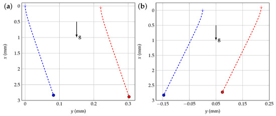
Figure 6. Deviations of the fall trajectories of two spheres in hydrodynamic interaction. (a) Trajectories of the two sphere when the blue one (${\mathcal{C}}_1$) is initially positioned above the red one (${\mathcal{C}}_2$). (b) Reverse situation of (a).

The influence of a vertical shift between the two spheres on their relative motion was also analyzed. For example, if sphere (1) is initially positioned above sphere (2), then during its movement, (1) displaces the fluid by pushing the fluid in front of it, and consequently, sphere (2) is deflected to the right, as shown in Figure 6a. The deflections are reversed when sphere (1) is positioned below sphere (2), as shown in Figure 6b.

The accuracy and convergence of the IIR-Filter method are now examined by comparing the numerical results obtained with those resulting from other analytical and/or numerical techniques available in the literature [7,9,13]. In [7], the authors determined the motion created in a viscous fluid at rest at infinity using two solid spheres moving with small, constant, and equal velocities, parallel to their center line. Their solution is based on the determination of the Stokes current function for the movement of the fluid. The forces required to maintain the motion of the spheres were then calculated. In the case of identical spheres, the forces are equal, and their modulus F is written as follows:

$$F=6\pi {\mu }_{f}r{\lambda }_{\Vert }{\mathrm{V}}_s^0$$

(22)

where $r=a/sinh\alpha$. The ratio $r/2a$ of the distance between the centers of the two spheres to their diameter is written here as $cosh\alpha$. According to [9], the coefficient ${\lambda }_{\Vert }$ can be written in the following form, which we denote as ${\lambda }_{\Vert }^B$:

$${\lambda }_{\Vert }^B=\frac{4}{3}sinh\alpha \sum _{n=1}^{\infty }\frac{n(n+1)}{(2n-1)(2n+3)}\left[1-\frac{4{sinh}^2\left(n+\frac{1}{2}\right)\alpha -{(2n+1)}^2{sinh}^2\alpha }{2sinh(2n+1)\alpha +(2n+1)sinh2\alpha }\right]$$

(23)

Thus, ${\lambda }_{\Vert }$ represents the ratio between the force required to maintain the motion of one sphere in the presence of the other and the force necessary to maintain its motion with the same velocity if the other sphere was at an infinite distance. Figure 7 shows the evolution of the drag correction factor ${\lambda }_{\Vert }$ of the two spheres when falling parallel to the line connecting their centers.

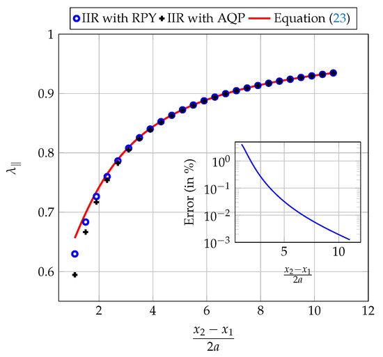
Figure 7. Evolution of the drag correction factor ${\lambda }_{\Vert }$ of the two spheres falling parallel to the line connecting their centers.

In the case of the motion of the two spheres being perpendicular to the line of their centers, Goldman et al. [8] found the following empirical formula:

$${\lambda }_{\perp }^G=1-\frac{3}{4}\xi +\frac{9}{16}{\xi }^2-\frac{59}{64}{\xi }^3+\frac{465}{256}{\xi }^4-\frac{15813}{7168}{\xi }^5+2\frac{{\xi }^6}{1+\xi }$$

(24)

where $\xi =a/(y_2-y_1)$.

The results obtained agree with those of Brenner [9] for large separation distances in front of the diameter $d=2a$ of the spheres. In this case, the relative error is less than ${10}^{-2}\%$. On the other hand, the relative error increases and becomes non-negligible as the separation distance between the two particles decreases. This behavior is explained by the influence of near-field interactions (lubrication effect), which are not properly taken into account in the mobility matrix.

Figure 8 shows the evolution of the drag correction factor ${\lambda }_{\perp }$ for two spheres falling perpendicular to the line connecting their centers. The results obtained using the chosen resolution method, with the use of the RPY approximation, are consistent with those of Goldman et al. [8] (refer to the insert in Figure 6 showing the relative error in %, defined as $|{\lambda }_{\perp }^{\mathrm{IIR}}-{\lambda }_{\perp }^G|\times 100/{\lambda }_{\perp }^G$) for the sedimentation of two identical spherical particles in a perpendicular direction at the line connecting their centers.

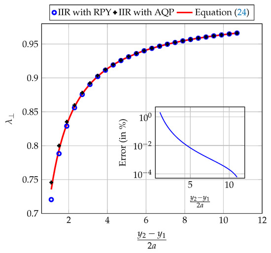
Figure 8. Evolution of the drag correction factor ${\lambda }_{\perp }$; the two spheres fall perpendicular to the line connecting their centers.

The relative error calculated in the case of the parallel fall is greater than that calculated in the perpendicular situation. The physical origin of this difference is due to the fact that in the first case, the dynamics of the particles downstream are strongly influenced by the disruption of the flow caused by the sphere upstream, just as when a ship moves in the wake of another rather than alongside it.

As shown both in Figure 7 and Figure 8, the numerical results obtained by IIR filters are consistent with those obtained analytically for relatively large separation distances, as noted above. In the case of small separation distances, where deviations from analytical results are more pronounced, we found that the results obtained with the IIR-Filter method are very close to those obtained with the Euler method for the two approximations considered here (QPA and RPY). The observed discrepancies are therefore due more to the limitations of the QPA and RPY approximations than to the calculation methods. We therefore proposed in this work to correct the RPY mobility matrix in order to obtain better results at low separation distances.

3.3. Correction to the RPY Mobility Matrix

In order to correct the deviations observed at small separation distances, we propose to introduce, in the RPY mobility matrix, a corrective term of an order greater than 2 into $a/r_{12}$. The corrected matrix ${}_{\mathrm{RPY}}\left(\mathcal{M}\right)^c$ is thus written as

$$\left|\begin{array}{cc}\hfill {}_{\mathrm{RPY}}\mathcal{M}_{11}^c={}_{\mathrm{RPY}}\mathcal{M}_{22}^c& =\frac{{\mathbb{I}}_3}{6\pi {\mu }_{f}a}\hfill \\ \hfill {}_{\mathrm{RPY}}\mathcal{M}_{12}^c={}_{\mathrm{RPY}}\mathcal{M}_{21}^c& =\frac{1}{8\pi {\mu }_f{r}_{12}}\left\{\left[1+\frac{2a^2}{3r_{12}^2}-\alpha \left(r_{12}\right)\frac{2a^3}{r_{12}^3}\right]{\mathbb{I}}_3\right.\hfill \\ \hfill & +\left.\left[1-\frac{2a^2}{r_{12}^2}-\alpha \left(r_{12}\right)\frac{2a^3}{r_{12}^3}\right]\frac{{\mathbf{r}}_{\mathbf{12}}·{\mathbf{r}}_{\mathbf{12}}}{r_{12}^2}\right\}\hfill \end{array}\right.$$

(25)

where $\alpha \left(r_{12}\right)$ is a corrective function. The aim of the present correction is to minimize the discrepancy between our numerical results obtained using the RPY approximation and the analytical results of both H. Brenner [9], in the case of the motion of the two particles parallel to the axis connecting their centers, and of Goldman et al. [8], in the case of perpendicular motion.

The expression of the function $\alpha \left(r_{12}\right)$ should be determined as a function of the separation distance $r_{12}$. This function reduces the discrepancy between the results of the present study and the analytical solutions [8,9] for a given separation distance of $r_{12}$. Figure 9 shows the $\alpha$ values leading to a minimum error for a given value of $\zeta =2a/r_{12}$.

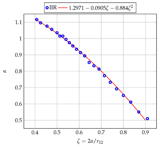
Figure 9. Variation in the corrective function $\alpha$ as a function of $\zeta =2a/r_{12}$.

An interpolation of the results shown in Figure 9 led to the following expression of $\alpha$ as a function of the parameter $\zeta =2a/r_{12}$, with a regression coefficient $R^2=0.998$:

$$\alpha \left(\zeta \right)=1.2971-0.0905\zeta -0.884{\zeta }^2$$

(26)

The numerical IIR-Filter solution of the two-particle sedimentation problem with hydrodynamic interactions was repeated using the corrected mobility matrix (25), with the $\alpha$ expression (26). As can be seen from Figure 10a,b, the introduced correction considerably improves the correspondence between numerical and analytical results, which confirms its relevance and allows the lubrication effect to be integrated very simply into the RPY mobility matrix.

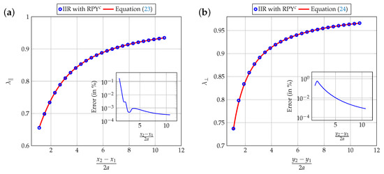
Figure 10. Evolution of the drag correction factor $\lambda$: (a) the two spheres’ sediment parallel to the line connecting their centers; (b) the two spheres’ sediment perpendicular to the line connecting their centers. The generalized mobility matrix used is given by (25).

4. Sedimentation of Three Particles

The study of the sedimentation of a triplet of particles (see Figure 11) is discussed here. The three identical spherical particles can be arranged evenly or irregularly. The literature examines these different configurations [13,31,32].

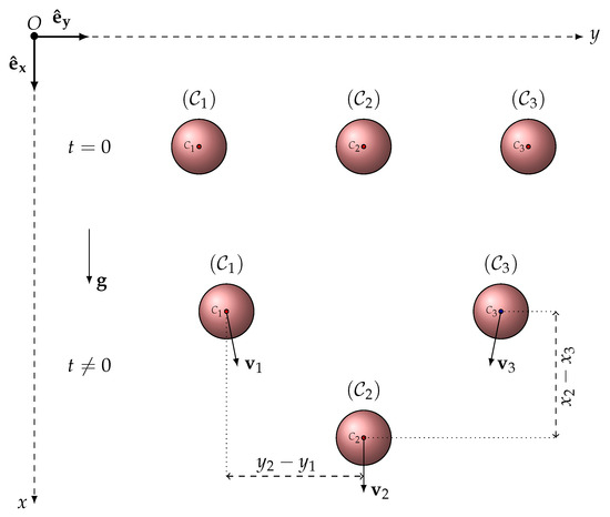
Figure 11. Three particles sedimenting in a viscous fluid at rest.

In the first configuration, the three spheres are positioned in such a way as to be equidistant along the horizontal axis, with a distance equal to $6a$ between each particle. The particle, initially at the center of this configuration, moves during sedimentation, at a higher speed than the two spheres positioned at the ends. It drags the two extreme spheres with it, causing them to come together.

Figure 12 illustrates the trajectories of the three particles obtained using the IIR-based resolution method with the corrected RPY mobility matrix. The velocities of the two particles ($C_1$) and ($C_3$) increase as they approach and exceed the velocity of the sphere ($C_2$). This pair of particles then approaches the sphere ($C_2$) until it reaches a critical distance, as described by Ganatos [13].

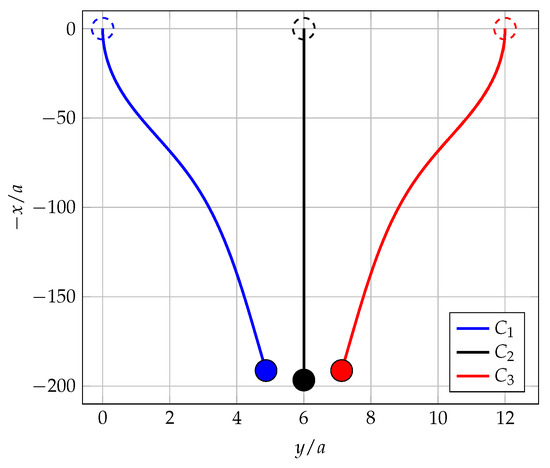
Figure 12. Trajectories of the three sedimenting particles.

The numerical results for this configuration are compared with those obtained by Ganatos et al. [13] who solved the steady-state creeping-motion governing equations of the flow (Stokes equation and mass conservation) for three sedimenting spheres. Figure 13 illustrates the variation in the horizontal distance $y_{21}$ between one of the extreme spheres (1 or 3) and the central sphere (2) as a function of dimensionless time $t^{*}=V_s^{0}t/a$.

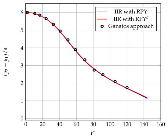
Figure 13. Evolution of $\left(y_2-y_1\right)/a$ as a function of dimensionless time $t^{*}=V_s^{0}t/a$. The symbols (circles) show the results obtained by Ganatos et al. [13] (reproduced with permission from Peter Ganatos, Robert Pfeffer, Sheldon Weinbaum published by Cambridge University Press, 2024).

Figure 14 shows the temporal variation in the vertical distance $x_{21}$ between one of the spheres at the ends and the central sphere. The results obtained from previous research conducted by Ganatos et al. [13] are included in both cases.

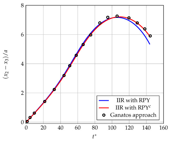
Figure 14. Evolution of $\left(x_2-x_3\right)/a$ as a function of dimensionless time $t^{*}=V_s^{0}t/a$. The symbols (circles) show the results obtained using the results of Ganatos et al. [13] (reproduced with permission from Peter Ganatos, Robert Pfeffer, Sheldon Weinbaum published by Cambridge University Press, 2024).

The comparison between the numerical results of this study and the results of Ganatos et al. [13] reveals a global agreement in the analytical and numerical evolutions of the distances between the particles. For $t^{*}⩽100$, the curves overlap almost perfectly. However, discrepancies appear beyond $t^{*}>100$, when the correction factor in the mobility matrix is not integrated. These differences are greatly reduced when the corrective function is integrated into the same matrix, thus confirming the effectiveness of the lubrication correction we introduced.

Figure 15 shows the temporal evolution of the vertical velocities of the three particles obtained using the IIR-Filter method, using the ${\mathrm{RPY}}^c–$corrected mobility matrix.

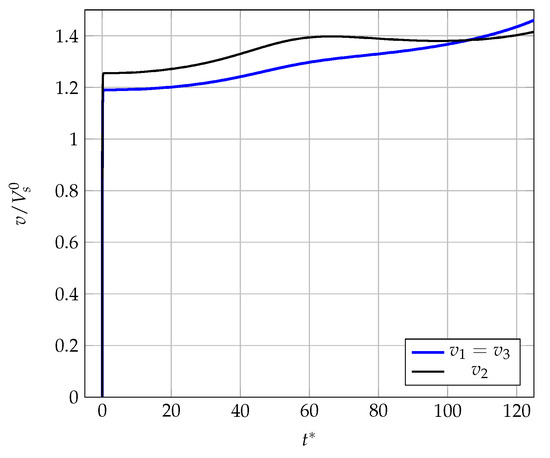
Figure 15. Velocity of the three particles obtained using the IIR-Filter method with the corrected mobility matrix RPY^c.

The velocity of the central sphere remains higher than those of the two extreme spheres, up to $t^{*}=106$. From this point on, the particle doublet gradually approaches the central sphere until it reaches the critical distance. The physical explanation for this strange behavior lies in the hydrodynamic interactions between the three spheres. Initially, the ${\mathrm{C}}_2$ sphere is pushed forward by ${\mathrm{C}}_1$ and ${\mathrm{C}}_3$ through the hydrodynamic interactions (incompressible fluid). As a result, ${\mathrm{C}}_2$ falls faster than ${\mathrm{C}}_1$ and ${\mathrm{C}}_3$. Before $t^{*}$, spheres C₁ and C₃ are disturbed by the wake of sphere C₂, and approach each other, forming a doublet, and its fall velocity gradually increases (see Figure 5 and Figure 15) until it equals that of C2 at $t=t^{*}$. Finally, for $t>t^{*}$, the doublet passes C₁ and continues to accelerate. According to the results of Ganatos et al. [13], the value of $t^{*}$ at which the vertical velocities of the three particles become equal is $107.8$. This represents a deviation of $1.6\%$ from the results obtained with the IIR-Filter method based on the corrected RPY mobility matrix, thus confirming the relevance of both the lubrication correction we calculated and of the IIR-Filter method.

5. Conclusions

The sedimentation dynamics ordinary differential equations (ODEs) of a number $N>1$ of colloidal particles (PCs), coupled by hydrodynamic interactions and suspended in an incompressible, unbounded Newtonian fluid, were numerically solved in this study for the first time using infinite impulse response recursive filters (the IIR-Filter method). The $N=2$ and $N=3$ cases were analyzed in detail, and many analytical and numerical results already established with other approaches were accurately found numerically using the IIR-Filter method.

An effective correction to the mobility matrix was also proposed in this work, within the framework of the Rotne–Prager–Yamakawa (RPY) approximation. This correction takes better account of hydrodynamic interactions between colloidal particles in the near-field (lubrication phenomenon at low inter-particle separations). This correction significantly improves the accuracy of the numerical results provided by the RPY approximation in the case of two and three particles. The theoretical results, obtained by directly solving the partial differential equations (PDEs) of the Stokesian dynamics of the fluid flowing around the colloidal particles moving in it, can then be recovered with great precision by solving the PCs’s ODEs with the mobility matrix approach.

The range of applications for the present approach is vast, and could extend, for example, to the study of microrheology or the drying of complex suspensions.

References

- Wacholder, E.; Sather, N.F. The hydrodynamic interaction of two unequal spheres moving under gravity through quiescent viscous fluid. J. Fluid Mech. 1974, 65, 417–437. [Google Scholar] [CrossRef]
- Brady, J.F.; Bossis, G. Stokesian Dynamics. Annu. Rev. Fluid Mech. 1988, 20, 111–157. [Google Scholar] [CrossRef]
- Sierou, A. Handbook of Materials Modeling; Chapter Stokesian Dynamics Simulations for Particle Laden Flows; Springer: Berlin/Heidelberg, Germany, 2005; pp. 2607–2617. [Google Scholar]
- Laura, S.; Paul, B. Colloidal dynamics in polymer solutions: Optical two-point microrheology measurements. Faraday Discuss. 2003, 123, 323–334. [Google Scholar] [CrossRef][Green Version]
- Waigh, T.A. Microrheology of complex fluids. Rep. Prog. Phys. 2005, 68, 685. [Google Scholar] [CrossRef]
- Lahboub, D.; Heyd, R.; Bakak, A.; Lotfi, M.; Koumina, A. Solution of Basset integro-differential equations by IIR digital filters. Alex. Eng. J. 2022, 61, 11899–11911. [Google Scholar] [CrossRef]
- Margaret, S.; George, B.J. The Motion of Two Spheres in a Viscous Fluid. Proc. R. Soc. A Math. Phys. Eng. Sci. 1926, 111, 110–116. [Google Scholar]
- Goldman, A.J.; Cox, R.G.; Brenner, H. The slow motion of two identical arbitrarily oriented spheres through a viscous fluid. Chem. Eng. Sci. 1966, 21, 1151–1170. [Google Scholar] [CrossRef]
- Brenner, H. The slow motion of a sphere through a viscous fluid towards a plane surface. Chem. Eng. Sci. 1961, 16, 242–251. [Google Scholar] [CrossRef]
- Guyon, E.; Hulin, J.P.; Petit, L.; Mitescu, C. Physical Hydrodynamics, 2nd ed.; Oxford University Press: Oxford, UK, 2015. [Google Scholar] [CrossRef]
- O’Neill, M. Some Motions in Incompressible Liquid Generated by the Movement of Spheres; University of London: London, UK, 2013. [Google Scholar]
- Wakiya, S. Slow Motions of a Viscous Fluid around Two Spheres. J. Phys. Soc. Jpn. 1967, 22, 1101–1109. [Google Scholar] [CrossRef]
- Ganatos, P.; Pfeffer, R.; Weinbaum, S. A numerical-solution technique for three-dimensional Stokes flows, with application to the motion of strongly interacting spheres in a plane. J. Fluid Mech. 1978, 84, 79–111. [Google Scholar] [CrossRef]
- Gluckman, M.J.; Pfeffer, R.; Weinbaum, S. A new technique for treating multiparticle slow viscous flow: Axisymmetric flow past spheres and spheroids. J. Fluid Mech. 1971, 50, 705–740. [Google Scholar] [CrossRef]
- Leichtberg, S.; Pfeffer, R.; Weinbaum, S. Stokes flow past finite coaxial clusters of spheres in a circular cylinder. Int. J. Multiph. Flow 1976, 3, 147–169. [Google Scholar] [CrossRef]
- Dhont, J.K.G. An Introduction to Dynamics of Colloids; Elsevier: Amsterdam, The Netherlands, 1996. [Google Scholar]
- Davies, C.N.L. Low Reynolds Number Hydrodynamics, with Special Applications to Particulate Media: John Happel and Howard Brenner; Second revised Edition; Noordhoff International Publishing: Leyden, IL, USA, 1973. [Google Scholar]
- O’neill, M.E.; Majumdar, R. Asymmetrical slow viscous fluid motions caused by the translation or rotation of two spheres. Part I: The determination of exact solutions for any values of the ratio of radii and separation parameters. Z. Angew. Math. Phys. ZAMP 1970, 21, 164–179. [Google Scholar] [CrossRef]
- Shing, B.C.; Xiangnan, Y. Faxen’s Laws of a Composite Sphere under Creeping Flow Conditions. J. Colloid Interface Sci. 2000, 221, 50–57. [Google Scholar] [CrossRef]
- Wajnryb, E.; Mizerski, K.A.; Zuk, P.J.; Szymczak, P. Generalization of the Rotne–Prager–Yamakawa mobility and shear disturbance tensors. J. Fluid Mech. 2013, 731, R3. [Google Scholar] [CrossRef]
- Zuk, P.J.; Wajnryb, E.; Mizerski, K.A.; Szymczak, P. Rotne–Prager–Yamakawa approximation for different-sized particles in application to macromolecular bead models. J. Fluid Mech. 2014, 741, R5. [Google Scholar] [CrossRef]
- Kim, S.; Mifflin, R.T. The resistance and mobility functions of two equal spheres in low-Reynolds-number flow. Phys. Fluids 1985, 28, 2033–2045. [Google Scholar] [CrossRef]
- Jeffrey, D.J.; Onishi, Y. Calculation of the resistance and mobility functions for two unequal rigid spheres in low-Reynolds-number flow. J. Fluid Mech. 1984, 139, 261–290. [Google Scholar] [CrossRef]
- Lamb, H. Hydrodynamics; Cambridge University Press: Cambridge, UK, 1932. [Google Scholar]
- Perkins, G.S.; Jones, R.B. Hydrodynamic interaction of a spherical particle with a planar boundary: II. Hard wall. Phys. A Stat. Mech. Its Appl. 1992, 189, 447–477. [Google Scholar] [CrossRef]
- Beenakker, C.W.J.; Van Saarloos, W.; Mazur, P. Many-sphere hydrodynamic interactions: III. The influence of a plane wall. Phys. A Stat. Mech. Its Appl. 1984, 127, 451–472. [Google Scholar] [CrossRef]
- van Saarloos, W.; Mazur, P. Many-sphere hydrodynamic interactions: II. Mobilities at finite frequencies. Phys. A Stat. Mech. Its Appl. 1983, 120, 77–102. [Google Scholar] [CrossRef]
- Heyd, R. Real-time heat conduction in a self-heated composite slab by Padé filters. Int. J. Heat Mass Transf. 2014, 71, 606–614. [Google Scholar] [CrossRef]
- Lotfi, M.; Mezrigui, L.; Heyd, R. Study of heat conduction through a self-heated composite cylinder by Laplace transfer functions. Appl. Math. Model. 2016, 40, 10360–10376. [Google Scholar] [CrossRef]
- Ambardar, A. Analog and Digital Signal Processing, 2nd ed.; Brooks/Cole: Pacific Grove, CA, USA, 1999. [Google Scholar]
- Durlofsky, L.; Brady, J.F.; Bossis, G. Dynamic simulation of hydrodynamically interacting particles. J. Fluid Mech. 1987, 180, 21–49. [Google Scholar] [CrossRef]
- Chauvin, C. Influence des Forces D’interactions Particulaires dans la Simulation Lagrangienne du Comportement de Particules en Sédimentation et Écoulements Turbulents. Ph.D. Dissertation, University of Rouen, Rouen, France, 1991. [Google Scholar]
Disclaimer/Publisher’s Note: The statements, opinions and data contained in all publications are solely those of the individual author(s) and contributor(s) and not of MDPI and/or the editor(s). MDPI and/or the editor(s) disclaim responsibility for any injury to people or property resulting from any ideas, methods, instructions or products referred to in the content. |
© 2024 by the authors. Licensee MDPI, Basel, Switzerland. This article is an open access article distributed under the terms and conditions of the Creative Commons Attribution (CC BY) license (https://creativecommons.org/licenses/by/4.0/).