Abstract
The basic approach of this research is to use an estimated series of effective reproduction number and multiple series of index from Oxford COVID-19 Government Response Tracker (OxCGRT) to measure the effect of Japanese government’s response on COVID-19 epidemic by running a time-varying regression with flexible least squares method. Then, we use estimated series of time-varying coefficients obtained from the previous step as proxy variables for the government response’s effect and run stepwise regressions with policy indicators of OxCGRT to identify which specific policy can mitigate the spreading of the COVID-19 epidemic in Japan. The main finding is that the response of Japanese government on COVID-19 epidemic is basically effective. However, the effect of Japanese government’ policy is gradually weakening. Under our identification scheme, we find that policies of quarantine and movement restrictions are still most effective, but policies of public health system do not show much effectiveness in the regression analysis. Another important empirical finding is that policies of economic support are effective in reducing the spread of COVID-19. Within the framework of empirical strategy proposed in this paper, the conclusion should be explained in the context of the socio-political and health situation in Japan, but the methodology is assumed to be applicable to other countries and regions in the analysis of government performance of response to COVID-19.
1. Introduction
The COVID-19 epidemic, which happened in Wuhan, China, in late 2019, has grown and spread rapidly and has became a global crisis. As of the end of May 2021, this serious pandemic has caused 172 million infections and 3.69 million deaths worldwide (Real-time statistics of COVID-19 can be confirmed at WHO Coronavirus (COVID-19) Dashboard (https://covid19.who.int, accessed on 1 June 2021). Based on current knowledge, the available vaccines can provide effective protection from the infection of COVID-19 but are unable to block the transmission completely. In an international context in which there are enormous differences from the point of view of vaccination coverage, it is difficult to hypothesize that the vaccination campaign could have a drastic effect in the short-medium time on the spread of COVID-19. Non-pharmaceutical interventions (NPIs), such as social distance, lockdown, and travel restrictions, are still the government’s main means of controlling COVID-19 infections. [] provides the projection of the transmission dynamics of COVID-19 in the U.S., which shows that COVID-19 will last quite long and prolonged or intermittent social distancing may be necessary into 2022.
For the situation of Japan, by the end of May 2021, Japan had already experienced four periods of rapid spread of infection. The Japanese government has already issued “Declaration of State of Emergency” three times to prevent the spread of the infection. The first time of Declaration of State Emergency was from 7 April 2020 to 25 May 2020, and the second time was from 8 January 2021 to 21 March 2021. The third time of emergency state was implemented on 25 April 2021 and is expected to continue until 20 June 2021. For the comprehensive summary of government response on COVID-19 pandemic in Japan, please refer to the homepage of Cabinet Secretariat of Japanese government (https://corona.go.jp/en/, accessed on 1 June 2021). At the time of submission of this article, the emergency declaration has been extended until 20 July. During the period of emergency state, Japanese government takes various measures, such as short-time business requests, school closure requests, and event restrictions, to stop the spread and prevent the resurgence of COVID-19 pandemic. Given that the epidemic situation in Japan is still severe, and the declaration of emergency state has been repeatedly extended, it is very necessary to explore whether the Japanese government’s response to the COVID-19 epidemic is indeed effective. In addition, we also want to know whether the effect of the Japanese government’s response to the epidemic has changed over time and identify which specific policy is effective in controlling the epidemic. To answer these questions, in this paper, we conduct a case study of Japan to evaluate its government response on COVID-19. Specifically, we take a time-varying regression approach to measure the effect of government response on COVID-19 pandemic in Japan and use the stepwise regression to identify the effect of specific policy.
Generally speaking, number of infected cases can be used to measure the severity of epidemic, but it may be not suitable for regression analysis due to its non-stationarity. We use a real-time estimation of effective reproduction number to measure the severity of the COVID-19 epidemic in Japan. Details about the data of will be given in Section 2.1. , which is a key concept in the epidemiology, is defined as the average number of secondary cases produced by a primary case. generally changes over time due to the change of susceptible individuals, as well as changes in control measures and other related factors. Another important concept in epidemiology is basic reproduction number , which measures the average number of secondary cases produced by a primary case when the whole population is given as susceptible individuals. There are two broad approaches that can be used to estimate in real time. One approach to estimate is to specify an epidemiological model and derive explicitly from model. Typical works, such as [,,,] take this approach. Refs. [,,] are typical works of another approach that is to use the information of serial interval (SI) of infectious disease. Ref. [] proposed a Bayesian method to estimate , and [] implemented this method in an R package EpiEstim. Refs. [,,] provide the general introduction of estimation of . Recently, ref. [] derived from a standard SIR model and estimated it with Kalman filter. Estimation with Kalman filter can use full-sample information without statistical parameter tuning.
To measure the government response quantitatively, we use the Oxford COVID-19 Government Response Tracker (OxCGRT). Details of OxCGRT can be found in [] and the related web pages (https://github.com/OxCGRT/covid-policy-tracker, https://www.bsg.ox.ac.uk/research/research-projects/covid-19-government-response-tracker and https://github.com/OxCGRT/covid-policy-tracker/blob/master/data/OxCGRT_latest.csv, accessed on 1 June 2021). OxCGRT tracks various anti-epidemic policies and categorizes them into four categories, containment and closure policies, economic policies, health system policies, and miscellaneous policies, and record these policies as policy indicators in the form of ordinal scale or U.S. dollars. Economic policies are recorded as the actual spending. From 12 June 2021, vaccination policies are added to the OxCGRT Version 3.01. In addition, OxCGRT summarizes these policies by providing 4 kinds of composite index, government response index, containment and health index, stringency index, and economic support index. Stringency index represents the stringency of various containment and closure policies. Containment and health index evaluate both health system policies and containment and closure policies. Among the 4 kinds of index, government response index is the most comprehensive. In addition to the various policies mentioned above, it also includes economic support policies. Table 1 summarizes the policy indicators and indices used in this paper.

Table 1.
OxCGRT index and policy indicator.
Given the appropriate data that can measure the severity of the COVID-19 epidemic and the corresponding government response, our method of this paper is a case study of Japan’s government response to COVID-19. We conduct time-varying regression analysis between effective reproduction number and the OxCGRT indices. The fixed parameter regression model can only estimate the average effect of the independent variable on the dependent variable within the sample period, but the time-varying parameter model can obtain the real-time effect. By investigating the time-varying coefficients, we can get better visualization about the effect of government response on COVID-19 epidemic. After obtaining the time-varying coefficients, we run stepwise regression with time-varying coefficients on the policy indicators provided by OxCGRT to identify which specific policy is effective in controlling the spread of COVID-19 infections. The reason that we use stepwise regression is that, if we use all policy indicators as independent variables in one regression, multicollinearity in the data of policy indicators makes the regression unfeasible. We need to find the best combination of independent variables. Stepwise regression is a smart way to determine the best combination of regressors. Our empirical strategy is summarized in Figure 1.
Figure 1.
Empirical strategy.
In this paper, although we take Japan as the research object, the methodology adopted in this paper is also applicable to other countries and regions. For related literature, [] uses the cross-country panel data of . They use estimated by [] to measure the COVID-19 spread and OxCGRT to investigate the effects of a variety of NPIs used by governments to mitigate the spread of COVID-19. Panel data can capture the intrinsic differences between countries. In addition, the regression specification in [] can identify the effect of each specific control measure and provide a more detailed guidance for government when choosing the control measure. Ref. [] also provide the empirical evidence of NPIs in the sample of 14 European countries. Their analysis shows that NPIs can effectively reduce . Ref. [] also discuss the government performance and the factors that affect prediction of the success of national responses to COVID-19 and will influence future pandemic preparedness. In addition, investigating the effect of specific NPIs policies between different periods or regions also provides our some important insights. Ref. [] study the rate of growth of daily COVID-19 cases in all the Italian regions and find that reopening school dose accelerate the growth rate of COVID-19 infection. Compared to these related works, our approach does not focus on some specific NPIs policies but, rather, evaluating the government response to COVID-19 in a more general view.
The remainder of the study is organized as follows. Section 2 describes the data and regressions. Section 3 discusses the empirical results and related topics. Section 4 concludes this paper and gives the prospect for further research. It should be noted that research on COVID-19 epidemic is advancing day by day, and the conclusions of this paper are also tentative. With the accumulation of data, it will be necessary to reassess this topic in the future.
2. Empirical Analysis
2.1. Data
In our empirical analysis, the sample period is from 1 January 2020 to 31 May 2021. Figure 2 shows some basic statistics of COVID-19 in Japan that can be downloaded from the homepage of Ministry of Health, Labor, and Welfare (https://www.mhlw.go.jp/stf/covid-19/open-data.html, accessed on 1 June 2021). As we can confirm from these figures, there have been four periods when the infection has spread rapidly. The peak of the first wave came in April 2020. Following the first wave, the peaks of the second, third, and fourth waves are in August 2020, January 2021, and May 2021, respectively.
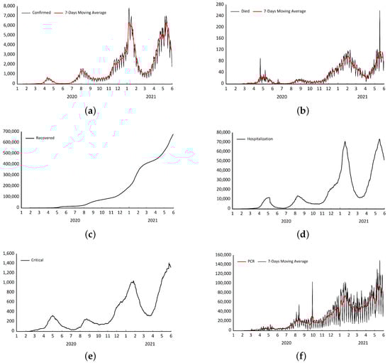
Figure 2.
Summary of COVID-19 pandemic in Japan. (a) Number of Daily New Confirmed Infected Cases. (b) Number of Daily New Confirmed Death Cases. (c) Number of Cumulative Recovered Cases. (d) Number of Patients in Hospitalization (e) Number of Critical Patients (f) Number of Daily PCR Testing Cases.
As we introduced in Section 1, the main data used in empirical analysis are , policy indicators, and 3 kinds of index provided by OxCGRT. OxCGRT index is given in Figure 3. We do not use economic support index in our empirical analysis because economic support generally does not directly control COVID-19 infections. The government provides economic support to the unemployed and companies to combat the recession caused by COVID-19 epidemic. Each specific policy indicator is given in Figure 4. The gray-shaded area shows the period of emergency state declared by Japanese government.
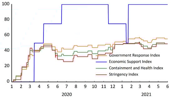
Figure 3.
OxCGRT index of Japanese government.
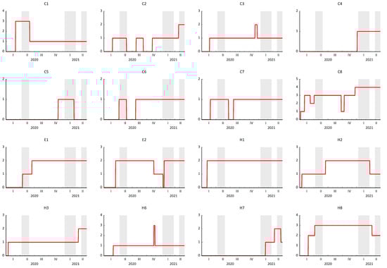
Figure 4.
OxCGRT policy indicator of Japanese government.
Table 1 summarizes the indices and policy indicators provided by OxCGRT. Index is calculated by aggregating corresponding policy indicators. For the details of calculation, please refer to the related Github page (https://github.com/OxCGRT/covid-policy-tracker/blob/master/documentation/index_methodology.md, accessed on 1 June 2021).
We use R package EpiEstim to estimate the from 15 February 2020 to 31 May 2021, which is given in Figure 5. We can also find obvious 4 peaks of infection spread from Figure 5. The data of daily infected cases used in the estimation of is collected from the Johns Hopkins CSEE repository (https://github.com/CSSEGISandData/COVID-19, accessed on 1 June 2021). When using EpiEstim, we must specify the serial interval (SI) of COVID-19 infection. [] fitted the data of 28 infector-infectee pairs on a log-normal distribution of serial interval and obtained the mean and standard deviation of serial interval as 4.7 days (95% confidence interval: 3.7 days, 6.0 days) and 2.9 days (95% confidence interval: 1.9 days, 4.9 days). For other important epidemiological features of COVID-19, ref. [] provide the a systematic review of COVID-19 based on current evidence.
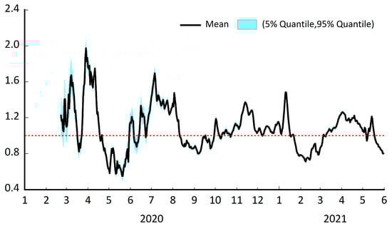
Figure 5.
estimated by EpiEstim.
Finally, we summarize the descriptive statistics of all data in Table 2. Augmented Dickey–Fuller (ADF) unit root test shows that all variables used in regression are stationary.
Table 2.
Summary statistics.
2.2. Regression Analysis
We use a simple log-log specification for time-varying regression. represents the disturbance term in regression equations.
represents the index series of OxCGRT. is the time-varying constant and is the time-varying coefficient. measures the effect of on , which can be explained as 1% change of can generate change of . Generally, means that the government response can mitigate the spread of epidemic by reducing . Note that, since the data series of is high series-correlated, it may be appropriate to include autoregression (AR) or moving average (MA) terms in the regression equation. However, our objective is not to find a time-series model that can fit well, but to find the statistical significance between and . When we treat and as fixed coefficients, we can obtain the values of coefficients by running an OLS regression. Results of OLS regression are given in Table 3. Given the negative value of coefficient on with 1% statistical significance, although regressions with government response measured by different indices and have small difference in the size of coefficients, it can be confirmed that the government response does have effect on reducing , which means that government response does reduce and slow down spread of the COVID-19 epidemic.
Table 3.
OLS regression of Equation (1).
These values measure the average effect of government response on fighting the COVID-19 epidemic during the whole sample period. At the same time, given the fact that the COVID-19 epidemic situation in Japan is still not in total control, we also want to know whether the effect of government response changes over time. Flexible Least Squares (FLS) approach proposed by [] is a convenient method to do this job. After obtaining the fixed coefficients of Equation (1) by running the OLS regression, we re-estimate this regression equation in a time-varying context. We can get 3 series of for which we have 3 kinds of OxCGRT index.
Figure 6 is the plot of time-varying coefficient estimated from the FLS regression of Equation (1). When the coefficients are below 0, it means that the government response can effectively reduce . During whole sample period, at most times, in Japan, the government response has some deterrent effect on the COVID-19 epidemic. However, deterrent changes over time. The gray-shaded area in Figure 6 indicates the period of emergency state in Japan. The deterrent effect of the 1st emergency state (7 April 2020–25 May 2020) is clearly stronger than the effect of the 2nd emergency state (8 January 2021–21 March 2021). Table 4 summarizes the average effect of emergency state on COVID-19 epidemic in Japan. The average effect of government response during the period of emergency state is evaluated as the average of regression coefficients during the corresponding period.
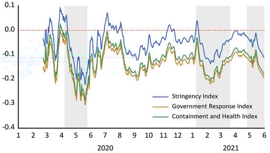
Figure 6.
Time-varying coefficient in regression of Equation (1).
Table 4.
Average effect of emergency state on the COVID-19 epidemic in Japan.
From the above analysis, it can be said that the Japanese government’s response on COVID-19 epidemic is basically effective. However, the effect of emergency state, which extends to the third time declaration, is gradually weakening. During the period of emergency state, the government is asking people to refrain from going out or traveling, but it is thought that people have become accustomed to long period of emergency state and have reached the limit of “patience”.
After obtaining , we use it as a dependent variable in the following regression equation with specific policy indicators. means the set of policy indicators. For example, is the time-varying coefficients obtained from the regression of on government response index, and, if we put all 16 policy indicators that are aggregated in government response index into the , multicollinearity existing in these policy indicators makes regression unfeasible. To avoid this difficulty, we use stepwise regression proposed by [] to choose the best subset of 16 policy indicators. If is negative and statistically significant, the corresponding policy indicator can be identified as an effective measure to control epidemic.
Table 5, Table 6 and Table 7 give the results of variable selection and corresponding regression. A policy indicator that has a statistically significant coefficients with negative sign is identified as effective policy. From these results, we find that, under our identification framework, not all policies may be effective in controlling the COVID-19 epidemic in Japan.
Table 5.
Stepwise regression of policy indicators in government response index.
Table 6.
Stepwise regression of policy indicators in containment and health index.
Table 7.
Stepwise regression of policy indicators in stringency index.
From the regression results in Table 5, we can find that C1 (school closing), C5 (close public transport), C6 (stay at home requirements), and C7 (restrictions on internal movement) are statistically significant as the effective policies. E1 (income support for households) and E2 (debt/contract relief for households) are also effective. The finding that economic support policies can reduce is worth noting. During the pandemic, many people lost jobs and had to go outside to find new jobs. Economic support, such as cash payment and debt relief, can reduce the risk of infection by helping households through difficult times. Actually, the Japanese government provided 100,000 yen in cash to all residents in 2020. The validity of this policy can also be confirmed from the above regression results.
H3 (contact tracing) and H8 (protection of elderly people) are identified as effective policies in the stepwise regression of policy indicators in containment and health index. As a specific example of H3, the Japanese government is actively encouraging the public to use the COVID-19 Contact-Confirming Application (https://www.mhlw.go.jp/stf/seisakunitsuite/bunya/cocoa_00138.html, accessed on 1 June 2021). This application tracks contacts with positive infections and reports those contacts to government agencies. In addition, to protect the elderly people, most elderly and medical facilities have severely restricted visits, given that elderly people infected with COVID-19 are more likely to become severely ill. Containment policies, such as C5 and C6, still show the significant effectiveness in this regression.
From the regression results showed in Table 7, we can find that containment policies, C5 (close public transport), C6 (stay at home requirements), and C7 (restrictions on internal movement), are still the most effective methods to control the spread of the COVID-19 epidemic. Especially, C5 (close public transport) and C6 (stay at home requirements) are two policies chosen in all 3 regressions of Equation (2). Note that, actually, in Japan, not all public transportation has been suspended. Public transportation is responding to the COVID-19 epidemic by suspending operations, reducing flights, and advancing the last train time at the request of the government. C6 (stay at home requirements) and C7 (restrictions on internal movement) are old-fashioned methods to control epidemic, but these methods are still the most effective. These methods limit the contact of people to each other and reduce the risk of infection. Note that, although we have differences among different regressions, we can summarize the common conclusion from these results. Containment policies are the most effective methods to control the COVID-19 epidemic.
3. Discussion of Empirical Results
Given the empirical results obtained from previous analysis, we can conclude that that the Japanese government’s response on COVID-19 epidemic is basically effective. However, the effect is gradually weakening. This can be visually confirmed from Figure 5. During the period of emergency state, the strategy of Japanese government to completely control COVID-19 epidemic through the self-restraint of people has a temporary effect, in the short term. However, given the fact that the period of emergency state is prolonged now, we have to say that its effectiveness is doubtful. The Japanese government is required to seek more effective strategies to control the epidemic based on the current laws and administrative system. At the same time, we should note that the conclusion must be explained in the context of the socio-political and health situation in Japan.
Recent research shows that the spread of COVID-19 can be affected by many other factors. Ref. [] ’s analysis shows that geographical and climatic factors, such as temperature, humidity, and latitude measurements, are consistent with the behavior of a seasonal respiratory virus. Ref. [] also confirms the seasonality in the spread of COVID-19. A further important variable is characterized by the chronic exposure of the population to atmospheric contamination which can affect the severity and spread of the virus. Refs. [,,] are typical works related to this topic. It is necessary to consider these factors when we evaluate the government performance of fighting COVID-19.
The statistical models specified in this paper are one possible alternative to evaluate the government response to COVID-19 and identify the effect of specific policy, but not the only one. Just as what we mentioned in the previous paragraph, seasonality, geographical, and climatic factors and environmental factors should be also considered. In the field of economics, causal identification methods, such as difference in difference (DID), propensity score matching, and discontinuity regression, have been widely used. Applying these methods to identify the effects of infectious disease control measures is expected to be an important research theme in the future.
4. Concluding Remarks
In this paper, we use the estimated effective reproduction number of the COVID-19 epidemic to measure the severity of it. In addition, we use the OxCGRT to measure the government response on COVID-19 epidemic. Our research objective is to figure out the effect of Japanese government’s response on COVID-19 epidemic.
The main methodology is regression analysis with and OxCGRT, including indices and policy indicators. We confirmed the average effect by OLS regression, which means that, on the whole, the Japanese government’s response to the epidemic is effective in curbing the spread of the epidemic. However, time-varying regression with FLS method shows that the effect is changing over time, specifically, gradually weakening. Finally, stepwise regression identifies the effect of specific policy. At the time of submission, the third emergency state is still ongoing, but the epidemic in Japan has not been fully controlled. The OxCGRT indices in Figure 3 show that the Japanese government’s response to the COVID-19 epidemic has not weakened, but the analysis in this article implies that the Japanese government needs to take more powerful measures to control the spread of this epidemic. The time-varying regression visualizes the effect of government response on COVID-19 in a consistent and comparable way, but this method is not suitable for comparison between different countries or regions. Panel data analysis, such as [] is more suitable in the context of international comparison.
Restricted by current laws and regulations, the Japanese government cannot restrict the freedom of citizens to a greater extent, and restrict the flow of people or other economic activities to curb the spread of the epidemic. The Japanese government has decided to hold the Olympic Games in July, so it is necessary to seek more effective strategies to control the epidemic based on the current laws and administrative system. Again, we have to note that the empirical results and related policy implications should be explained in the context of the statistical models proposed in this paper.
Funding
This research was funded by Rissho University Research Promotion and Regional Alliance Centre Fund for supporting Research and Education (Type 3).
Institutional Review Board Statement
Not applicable.
Informed Consent Statement
Not applicable.
Data Availability Statement
All data used in this research is publicly open data. Any further information will be available from the corresponding authors on request.
Conflicts of Interest
The author declares no conflict of interest.
References
- Kissler, S.M.; Tedijanto, C.; Goldstein, E.; Grad, Y.H.; Lipsitch, M. Projecting The Transmission Dynamics of SARS-CoV-2 through The Postpandemic Period. Science 2020, 368, 860–868. [Google Scholar] [CrossRef] [PubMed]
- Chowell, G.; Nishiura, H.; Bettencourt, L.M. Comparative estimation of The Reproduction Number for Pandemic Influenza from Daily Case Notification Data. J. R. Soc. Interface 2007, 4, 155–166. [Google Scholar] [CrossRef] [PubMed] [Green Version]
- Cazelles, B.; Champagne, C.; Dureau, J. Accounting for Non-stationarity in Epidemiology by Embedding Time-varying Parameters in Stochastic Models. PLoS Comput. Biol. 2018, 14, e1006211. [Google Scholar] [CrossRef] [PubMed] [Green Version]
- Kucharski, A.J.; Russell, T.W.; Diamond, C.; Liu, Y.; Edmunds, J.; Funk, S.; Flasche, S. Early Dynamics of Transmission and Control of COVID-19: A Mathematical Modelling Study. Lancet Infect. Dis. 2020, 20, 553–558. [Google Scholar] [CrossRef] [Green Version]
- Dehning, J.; Zierenberg, J.; Spitzner, F.P.; Wibral, M.; Neto, J.P.; Wilczek, M.; Priesemann, V. Inferring Change Points in the Spread of COVID-19 Reveals The Effectiveness of Interventions. Science 2020, 369, eabb9789. [Google Scholar] [CrossRef]
- Wallinga, J.; Teunis, P. Different Epidemic Curves for Severe Acute Respiratory Syndrome Reveal Similar Impacts of Control Measures. Am. J. Epidemiol. 2004, 160, 509–516. [Google Scholar] [CrossRef] [Green Version]
- Cori, A.; Ferguson, N.M.; Fraser, C.; Cauchemez, S. A New Framework and Software to Estimate Time-varying Reproduction Numbers during Epidemics. Am. J. Epidemiol. 2013, 178, 1505–1512. [Google Scholar] [CrossRef] [Green Version]
- Chinazzi, M.; Davis, J.T.; Ajelli, M.; Gioannini, C.; Litvinova, M.; Merler, S.; Vespignani, A. The Effect of Travel Restrictions on The Spread of The 2019 Novel Coronavirus (COVID-19) Outbreak. Science 2020, 368, 395–400. [Google Scholar] [CrossRef] [Green Version]
- Thompson, R.N.; Stockwin, J.E.; van Gaalen, R.D.; Polonsky, J.A.; Kamvar, Z.N.; Demarsh, P.A.; Cori, A. Improved Inference of Time-varying Reproduction Numbers during Infectious Disease Outbreaks. Epidemics 2019, 29, 100356. [Google Scholar] [CrossRef]
- Nishiura, H.; Chowell, G. The Effective Reproduction Number as A Prelude to Statistical Estimation of Time-dependent Epidemic Trends. In Mathematical and Statistical Estimation Approaches in Epidemiology; Springer: Dordrecht, The Netherlands, 2009; pp. 103–121. [Google Scholar]
- Chowell, G.; Brauer, F. The Basic Reproduction Number of Infectious Diseases: Computation and Estimation using Compartmental Epidemic Models. In Mathematical and Statistical Estimation Approaches in Epidemiology; Springer: Dordrecht, The Netherlands, 2009; pp. 1–30. [Google Scholar]
- Gostic, K.M.; McGough, L.; Baskerville, E.B.; Abbott, S.; Joshi, K.; Tedijanto, C.; Cobey, S. Practical Considerations for Measuring The Effective Reproductive Number, Rt. PLoS Comput. Biol. 2020, 16, e1008409. [Google Scholar] [CrossRef]
- Arroyo-Marioli, F.; Bullano, F.; Kucinskas, S.; Rondón-Moreno, C. Tracking R of COVID-19: A New Real-time Estimation Using The Kalman Filter. PLoS ONE 2021, 16, e0244474. [Google Scholar] [CrossRef]
- Hale, T.; Angrist, N.; Goldszmidt, R.; Kira, B.; Petherick, A.; Phillips, T.; Tatlow, H. A Global Panel Database of Pandemic Policies (Oxford COVID-19 Government Response Tracker). Nat. Hum. Behav. 2021, 5, 529–538. [Google Scholar] [CrossRef]
- Chen, L.; Raitzer, D.; Hasan, R.; Lavado, R.; Velarde, O. What Works to Control COVID-19? Econometric Analysis of a Cross-Country Panel; Asian Development Bank Economics Working Paper Series 625; Asian Development Bank: Metro Manila, Philippines, 2020. [Google Scholar]
- Abbott, S.; Hellewell, J.; Thompson, R.N.; Sherratt, K.; Gibbs, H.P.; Bosse, N.I.; Funk, S. Estimating the Time-varying Reproduction Number of SARS-CoV-2 using National and Subnational Case Counts. Wellcome Open Res. 2020, 5, 112. [Google Scholar] [CrossRef]
- Baum, F.; Freeman, T.; Musolino, C.; Abramovitz, M.; De Ceukelaire, W.; Flavel, J.; Villar, E. Explaining Covid-19 Performance: What Factors Might Predict National Responses? BMJ 2021, 372. [Google Scholar] [CrossRef]
- Casini, L.; Roccetti, M. Reopening Italy’s Schools in September 2020: A Bayesian Estimation of the Change in the Growth Rate of New SARS-CoV-2 Cases. medRxiv 2021. [Google Scholar] [CrossRef]
- Nishiura, H.; Linton, N.M.; Akhmetzhanov, A.R. Serial Interval of Novel Coronavirus (COVID-19) Infections. Int. J. Infect. Dis. 2020, 93, 284–286. [Google Scholar] [CrossRef] [PubMed]
- Park, M.; Cook, A.R.; Lim, J.T.; Sun, Y.; Dickens, B.L. A Systematic Review of COVID-19 Epidemiology based on Current Evidence. J. Clin. Med. 2020, 9, 967. [Google Scholar] [CrossRef] [PubMed] [Green Version]
- Kalaba, R.; Tesfatsion, L. Time-varying Linear Regression via Flexible Least Squares. Comput. Math. Appl. 1989, 17, 1215–1245. [Google Scholar] [CrossRef] [Green Version]
- Derksen, S.; Keselman, H.J. Backward, Forward and Stepwise Automated Subset Selection Algorithms: Frequency of Obtaining Authentic and Noise Variables. Br. J. Math. Stat. Psychol. 1992, 45, 265–282. [Google Scholar] [CrossRef]
- Sajadi, M.M.; Habibzadeh, P.; Vintzileos, A.; Shokouhi, S.; Miralles-Wilhelm, F.; Amoroso, A. Temperature, Humidity, and Latitude Analysis to Estimate Potential Spread and Seasonality of Coronavirus Disease 2019 (COVID-19). JAMA Netw. Open 2020, 3, e2011834. [Google Scholar] [CrossRef]
- De Natale, G.; De Natale, L.; Troise, C.; Marchitelli, V.; Coviello, A.; Holmberg, K.G.; Somma, R. The Evolution of COVID-19 in Italy after the Spring of 2020: An Unpredicted Summer Respite Followed by A Second Wave. Int. J. Environ. Res. Public Health 2020, 17, 8708. [Google Scholar] [CrossRef] [PubMed]
- Fattorini, D.; Regoli, F. Role of the Chronic Air Pollution Levels in The Covid-19 Outbreak Risk in Italy. Environ. Pollut. 2020, 264, 114732. [Google Scholar] [CrossRef] [PubMed]
- Conticini, E.; Frediani, B.; Caro, D. Can Atmospheric Pollution be Considered A Co-factor in Extremely High Level of SARS-CoV-2 Lethality in Northern Italy? Environ. Pollut. 2020, 261, 114465. [Google Scholar] [CrossRef] [PubMed]
- Domingo, J.L.; Rovira, J. Effects of Air Pollutants on The Transmission and Severity of Respiratory Viral Infections. Environ. Res. 2020, 187, 109650. [Google Scholar] [CrossRef] [PubMed]
Publisher’s Note: MDPI stays neutral with regard to jurisdictional claims in published maps and institutional affiliations. |
© 2021 by the author. Licensee MDPI, Basel, Switzerland. This article is an open access article distributed under the terms and conditions of the Creative Commons Attribution (CC BY) license (https://creativecommons.org/licenses/by/4.0/).