Abstract
This study introduces a novel forecast combination method for monthly Japanese tourism demand, analyzed at both aggregated and disaggregated levels, including tourist, business, and other travel purposes. The sample period spans from January 1996 to December 2018. Initially, the time series data were decomposed into high and low frequencies using the Ensemble Empirical Mode Decomposition (EEMD) technique. Following this, Autoregressive Integrated Moving Average (ARIMA), Neural Network (NN), and Support Vector Machine (SVM) forecasting models were applied to each decomposed component individually. The forecasts from these models were then combined to produce the final predictions. Our findings indicate that the two-stage forecast combination method significantly enhances forecasting accuracy in most cases. Consequently, the combined forecasts utilizing EEMD outperform those generated by individual models.
1. Introduction
The successful vaccination rollouts and coordinated lifting of travel restrictions are expected to boost consumer confidence and accelerate the recovery of international tourism. According to UNWTO, initial estimates suggest a 2% growth above 2019 levels. In the first seven months of 2024, international tourist arrivals reached 96% of pre-pandemic levels, indicating a near-full recovery (UNWTO, 2024). However, the central forecast depends on the pace of recovery in Asia and existing economic and geopolitical risks. Studies focused on improving the accuracy of tourism demand forecasts are important as these enable enhanced planning and better allocation of scarce resources (for e.g., rooms, transport, access to food, and security) for tourism purposes.
In this paper, we focus on evaluating the forecasting accuracy of EEMD technique and compare it with other forecasting models such as ARIMA, NN, and SVM. This study utilizes Japanese tourism demand data.
There are several reasons for considering Japan as a case study. First, Japanese tourism is particularly interesting because, traditionally, tourism was not strongly associated with Japan (Polunin, 1989). However, the implementation of the inbound travel promotion campaign, Visit Japan, in 2003 (Soshiroda, 2005), led to significant growth in tourist arrivals, with over 31 million tourist arrivals in 2018, a 263% increase since 2010 (UNWTO, 2019). Second, before the pandemic, travel and tourism were becoming major economic drivers for Japan, with the country experiencing some of the fastest inbound tourism growth rates in the world (Andonian et al., 2016). Despite the significant impact of the pandemic on global travel and tourism, Japan managed to maintain its global ranking within the sector. For instance, Japanese tourism demand had been increasing annually since the global financial crisis in 2009 (Yagasaki, 2021). Despite the ongoing pandemic, in 2020, Japan’s travel and tourism industry maintained its position as the third largest total contributor to GDP in the world. Third, tourism statistics indicate that the sector continues to be of significant importance to the Japanese economy, with the total contribution of travel and tourism to GDP being 4.7% of the total economy in 2020, while the total contribution of the sector to employment stood at 8.1% of total employment. Fourth, despite the continued growth in tourism demand since the global recession, research into forecasting Japanese tourism demand has been sparse. Finally, Yagasaki (2021) outlines several efforts by the Japanese government to revive tourism demand post-COVID-19. Accurate tourist arrivals forecasts are essential for safeguarding positive returns on significant investments in infrastructure and promotional activities, and for enabling policymakers to make informed decisions to boost economic development, well-being, and employment (Silva et al., 2019).
This study aims to provide insights into the effectiveness of combining EEMD with various forecasting models, using the dynamic and evolving context of Japanese tourism demand as a backdrop.
Interestingly, the majority of previous research has focused on Japanese outbound tourism and its impact on other economies (see, for example, Law (2001), Park et al. (2017), and Song et al. (2003)). In contrast, a recent attempt which directly tackles the issue of tourism demand for Japan is the work by W. Chen et al. (2017) through which they proposed a single dendritic neuron model for forecasting Japanese tourist arrivals. The authors found that their proposed model outperforms several other NN models. Russell (2017) performed a SWOT analysis for inbound Japanese tourism to provide policy recommendations to facilitate Japanese tourism industry, showing their effort in promoting Japanese tourism in line with the Japanese government’s aims and objectives. Many years ago, Turner et al. (1997) compared forecasts for inbound tourism to New Zealand, Australia, and Japan. Their findings showed the following: the periodic model is not a good candidate for tourism demand forecasting; there is no significant difference between the forecasts from a basic structural model and ARIMA; and the naïve model cannot be a substitute for seasonal integrated models. Accordingly, it is evident that there is a significant gap in the Japanese tourism demand forecasting literature in terms of methods considered and data that has been used. Japan’s tourism demand data is complex due to the presence of structural breaks and nonlinearity caused by the severe acute respiratory syndrome (SARS) outbreak in 2003, the Global Financial Crisis in 2008, the 2011 Japanese earthquake, tsunamis, and nuclear plant leakage incidents.
Since 2010, there has been an increase in the development and use of hybrid models and forecast combinations for tourism demand forecasting, and these have resulted in improved forecasting accuracy (Song et al., 2019). However, no single paper has evaluated the practical relevance and feasibility of a combination forecast for Japanese tourism demand. Therefore, our study aims to introduce a combination forecast which is based on a decomposition method and time series forecasting techniques. Here, we rely on a model based on Empirical Mode Decomposition (EMD) which is an adaptive decomposition method based on the original data. However, in comparison to other decomposition techniques like Wavelet Transform, EMD is affected by the modal aliasing effect. Therefore, in order to overcome this disadvantage, we employ EEMD, which is an extension of EMD that overcomes its limitations (Z. Wu & Huang, 2009). Thus, we propose decomposing the data with EEMD and then generating forecasts with SVM (Vapnik, 1998), NN, and classical ARIMA models, which are then combined, to predict Japanese tourism demand at an aggregated and disaggregated level based on the purpose of travel (tourism, business, and other). Forecasts from the proposed model are compared with several different linear and non-linear models as we seek to determine whether forecast combination improves the accuracy of overall forecasts. The evaluation of forecast combinations concerning Japanese tourist arrivals is important because research indicates that combined forecasts are preferable over univariate forecasts in many practical contexts (see, for example, Wong et al. (2007), G. Li et al. (2019), J. Wu et al. (2020)).
To the best of our knowledge, this is the first study that attempts to assess the EEMD method in the context of tourism. As indicated by the different degrees of seasonal R2 in Table 1, this study assesses the method using time series data with varying degrees of seasonality.

Table 1.
Summary statistics of monthly growth in arrivals.
The seasonal R2 in the last column was computed by regressing the first difference in the data against 12 monthly dummies. This paper makes several contributions to the tourism demand forecasting literature. Firstly, given the rapidly improving status of Japan as a key tourist destination, we extend knowledge about forecasting tourist arrivals in Japan which has been under-researched. Secondly, we are the first paper to propose a combination forecast for Japanese tourism demand. Thirdly, we introduce a new combination forecast by exploiting EEMD which is a powerful nonparametric method to decompose the time series of interest first and subsequently generate forecasts for decomposed components using SVM, ARIMA, and NN models to develop the forecast combination. This, in particular, is a timely and important innovation as forecast combinations are expected to further develop and play an increasingly significant role in the forecasting of tourism demand in future (Song et al., 2019, p. 356). Fourthly, this study provides forecasts for Japanese tourism demand at an aggregated and disaggregated level based on the purpose of travel (tourism, business, and other), which can be useful for stakeholders for the creation of better tailored policies for Japanese tourism. Finally, we hope this attempt sparks more interest by academics and practitioners to consider developing varied forecasting models to further improve the accuracy of Japanese tourism demand forecasts.
The remainder of this paper is organized such that Section 2 presents a concise literature review, Section 3 provides a brief description and methodology underlying EEMD, SVM, NN, and ARIMA models and presents a summary of the data, and Section 4 provides the forecast evaluation results. Section 5 concludes the study with results discussed.
2. Literature Review
We begin by presenting a concise review of the developments in forecast combination models in the context of tourism demand forecasting. Thereafter, we review the application of decomposition models for tourism demand forecasting. As reviewing all efforts at forecasting tourism demand is beyond the mandate of this paper, we refer those interested in a curated review of the tourism demand forecasting literature to Song et al. (2019) and Jiao and Chen (2019).
2.1. Forecasting Combination in Tourism Demand Forecasting
There is a growing importance of combination forecasting models in tourism. Recent evidence from the M4 competition indicated that forecast combinations can be very successful (Atiya, 2020). Nevertheless, in the context of tourism demand forecasting, the use of combination forecasts date back to the pioneering work by Fritz et al. (1984) who showed that forecast combination can result in smaller forecasting errors and overall accuracy improvements. Yet, in comparison to other disciplines, this is a short history (Gunter et al., 2020). A combination forecast can be defined as the following:
“An approach that generates a set of forecasts for the same demand variable by using different methods, and then combines these forecasts into one final, summarised forecast.”(Song et al., 2019, p. 354)
Song et al. (2019) identify several forecast combination methods in the context of the tourism demand literature. These include average-based methods using Pythagorean (arithmetic, geometric or harmonic) means; forecasting error-based methods; regression-based methods; and hierarchical methods, each with its own advantages and disadvantages.
A total of 17 of the key papers published on forecasting tourism demand with combination forecasts from 1984 to 2018 have been reviewed by Song et al. (2019). Therefore, instead of replicating the findings from these studies, we focus on reviewing tourism demand research with combination forecasts published since 2019.
G. Li et al. (2019) explored the potential of combining interval forecasts by combining different density forecasts from eight individual time series or econometric models in the context of Hong Kong’s inbound tourism demand. They find that combination forecasts are effective for producing accurate interval forecasts.
Sun et al. (2021) proposed a combination forecast based on time-varying jackknife model averaging with an application to Hong Kong tourist arrivals and showed that their proposed model outperforms the single model and three other combination methods in most cases. Liu et al. (2021) used simple average forecast combination to generate four combined models that included the combination of four time series models, three AI models, three hybrid Seasonal and Trend decomposition using Loess models and AI models, and the combination of all of the above ten models. They found the forecast combination with four time series models outperforming all other models used in this study. Kourentzes et al. (2021) showed that a forecast combination which combined a univariate model (exponential smoothing) with cross-sectional hierarchical forecasting techniques could outperform multivariate models when forecasting visitor arrivals from Africa pre-COVID.
Bekiroglu et al. (2022) proposed a dynamic ensemble algorithm for forecast combination and evaluated its performance via an application into tourist arrival forecasting. The algorithm runs a sparsification process to merge a subset of methodology space (which involved various univariate and multivariate forecasting algorithm) to avoid overfitting while improving out-of-sample accuracy.
Closely associated with forecast combinations is the development of hybrid forecasting models. To this end, classification techniques have been combined with various forecasting methods to develop hybrid models. For example, Genetic Algorithms (GA) are used to select the parameters in SVM within GA-Support Vector Regression models (Song et al., 2019). Those interested in classification forecasts in the context of tourism demand forecasting are referred to Pai et al. (2006) and Xu et al. (2016).
2.2. Decomposition Models in Tourism Demand Forecasting
Decomposition techniques such as filtering, spectral analysis, and EMD have been common applications for solving tourism demand problems (Bosupeng, 2019).
C. F. Chen et al. (2012) adopted an EEMD method and forecasted inbound international tourism demand to Taiwan. They found combined EEMD models superior in forecasting tourist arrivals to Taiwan relative to back-propagation NN alone. Lai et al. (2013) used a hybrid model that combined EMD and Support Vector Regression for forecasting tourist arrivals. Kummong and Supratid (2016) built a hybrid model combining discrete wavelet decomposition and a nonlinear autoregressive NN model with exogenous input for forecasting Thailand tourism and found it outperformed other related NN forecasts.
Silva et al. (2017) forecasted European tourism demand using nine models which included Singular Spectrum Analysis (SSA) and showed that the filtering technique of SSA was, on average, the best across all horizons. Yahya et al. (2017) used a hybrid modified EMD and NN model for tourism forecasting and showed that it outperforms NN and other EMD-NN models. G. Zhang et al. (2017) focused on improving the forecasting accuracy of daily occupancy for hotels by combining EEMD with ARIMA. They found this combination forecast produced more accurate results than ARIMA in the short run.
Silva et al. (2019) introduced a hybrid NN forecasting model for European tourist arrivals which incorporated decomposition with Singular Spectrum Analysis and showed that decomposition has the capability of significantly improving NN forecasts.
More recently, X. Li and Law (2020) used ensemble EMD for decomposing Google Trends and then applied several forecasting models to show that they could provide superior tourism demand forecasts. Xie et al. (2020) also employed the EMD method, incorporating adaptive noise, and showed that this model is effective for tourism forecasting at different horizons, based on both point and interval forecast comparisons.
Y. Zhang et al. (2021) proposed a deep learning method based on artificial intelligence for modeling tourism data which combines decomposition with deep learning. Tang et al. (2020) proposed a novel bivariate EMD approach, using data obtained by a search engine, for predicting tourist visits. An application into forecasting the tourist volume for an island province in Chian, Hainan, shows that this approach is significantly more accurate, and robust than several popular forecasting techniques.
Overall, the literature review has highlighted several gaps in academic research. First, none of the recent research in forecasting tourist arrivals sought to evaluate how developments in forecasting methodology and models (either univariate or multivariate) could impact forecasts for Japanese inbound tourism. Second, we did not uncover any studies that have evaluated the effectiveness of EEMD in relation to decomposing Japanese inbound tourism demand. Third, there exists no research that has sought to determine the impact of forecast combinations on the accuracy of Japanese tourism demand forecasts.
3. Methodology and Material
3.1. EEMD
EMD (Huang et al., 1998) is a relatively new nonparametric method that is not restricted by the assumptions of linearity or stationarity. The EMD technique decomposes time series into IMFs and a residual. In this section, we describe concisely the EMD algorithm as explained by Yeh et al. (2010a, 2010b) and applied by Fang et al. (2020). Accordingly, EMD is a nonparametric, adaptive method that is suitable for effectively capturing both non-stationarity and non-linearity behavior in time series data. In brief, the EMD technique deals with decomposing a time series into IMF with different frequencies and amplitudes. Z. Wu and Huang (2009) built on the limitations of the EMD technique and developed the improved EEMD approach which avoids the aliasing produced via EMD by adding a series of pure noise to the data set.
EEMD not only retains the adaptive nature of EMD but also introduces white noise to effectively avoid the problem of mode mixing, ensuring that the decomposed Intrinsic Mode Functions (IMFs) uniquely represent different time scales. In the context of forecasting, the limitations of EMD relative to EEMD are significant (Fang et al., 2020). EMD often suffers from mode mixing, where oscillations of different scales are not effectively separated, leading to misleading interpretations. This issue is mitigated in EEMD by adding white noise to the data, which helps to separate different scales more effectively and reduces the chance of mode mixing. Additionally, EMD is sensitive to noise, which can distort the decomposition process, whereas EEMD’s ensemble approach with added noise makes it more robust and reliable. EMD also struggles with end effects, where the decomposition near the boundaries of the data can be inaccurate. EEMD addresses this by averaging the results of multiple decompositions with different noise realizations, providing a more stable and accurate representation near the boundaries. Furthermore, EEMD is relatively simple compared to other combination methods, maintaining high prediction efficiency while ensuring a certain level of accuracy. These improvements make EEMD a superior choice for decomposing non-stationary and non-linear time series data, as demonstrated in the study by (Fang et al., 2020). The entire process can be summarized as the following procedure.
- Generate a new time series, by adding the original time series to a normally distributed white noise time series, :
- For the time series generated in (1), obtain the values of maximum and minimum.
- Employ an interpolation method and join the maximums to obtain the upper envelop and join all the minimum to generate the lower envelope.
- Compute the average of the upper and lower envelopes
- Obtain the mean deleted data, by subtracting the average computed in (2) from (1), the original time-series with added noise.
- If the IMF conditions are satisfied for , then repeat step one to step four until to achieve a monotonic function for the remainder. This procedure decomposes the original series into a remainder and a set of n independent IMFs, as shown below.
- Simulate a random time series of noise, and repeat step 2 to step 6, k-times.
- Finally, compute the means of the (k-times repeated) decomposed IMFs obtained in the previous steps.
The described EEMD technique is advantageous as the added random noise cancels in the end, and results in significantly reducing the likelihood of mode mixing. The decomposed series is finally denoted as the following:
where , in the above equation, is called the remainder and the n time series of represent the final IMFs. The following conditions must be met by IMFs:
- (1)
- Throughout the entire time scale, the difference between the number of maxima, minima, and zero crossings of the IMF should not be greater than 1.
- (2)
- At any given time, the mean value of the upper envelope and the lower envelope must be zero.
The remainder and the n independent IMFs obtained via EEMD preserves the main features of non-linearity and non-stationarity in the original data while avoiding the modal aliasing.
3.2. Support Vector Machine (SVM)
In contrast, SVM has the advantage of dealing with nonlinear regression estimation problems in many fields. It applies minimized structural risk principles to minimize an upper bound of generalization error (Pai et al., 2006). SVM belongs to the class of supervised machine learning algorithms that have proven successful at dealing with various practical problems, such as non-linear regression, non-linear time series, and pattern classification (Vapnik, 1998). SVM works by using a pre-selected kernel function to map the data into a multi-dimensional feature space. Next, this multi-dimensional space is used to construct the optimal classification plane which maximizes the distance between the hyperplane. As a technique that can be used for linear and non-linear forecasting, the SVM algorithm is as follows:
where is the weight coefficient and c is called the offset term. The Lagrangian function is then used to obtain the weights and the offset parameter in order to find the optimized solution for the following non-linear regression:
where and are the optimum parameters and is the non-linear kernel function.
3.3. Neural Networks (NN)
NN models are structured to include input, hidden, and output layers, which are connected by some weights. The NN algorithm adjusts the weights according to a learning method that minimizes a cost function to obtain the best fit to the data. Below, we provide a concise description of the NN estimation procedure.
- The inputs into hidden layer neuron j are combined, using a weighted linear combination, to obtain the input signal j:where is the threshold for the jth node and indicates the weight for jth neuron.
- Compute the output value from the hidden neuron node j, using a non-linear activation function:
- To start with, the weights, , take random values, and are then updated until minimizing a cost function such as Mean Square Errors (MSE), using the observed data.
3.4. Selection of Parameters
In this study, we utilized the radial basis kernel function in SVM. Grid search (Gridsearch), GA, and Particle Swarm Optimization (PSO) are employed in parameter optimization. The dimension of input vector is chosen from one to five, and then optimal parameters are obtained through the cross-intersection experiment by comparing the MSE.
For the NN model fitting, the training time was no more than 5000, the learning efficiency was set to 0.01, and the precision in training the network was chosen as 0.001. The Tansig and ‘logsig’ functions were selected as the activation function, and ‘trainlm’ and ‘traingd’ were chosen as the training functions. The number of nodes for each hidden layer varies from two to twelve. The activation function and the number of nodes are chosen by comparing Mean Square Prediction Errors (MSPE). To find the optimum number of parameters in ARIMA models, BIC criterion is used in this study.
The data employed in this paper were taken from Japan National Tourism Organization (JNTO). Our sample, in all cases, start from January 1996 to December 2018. We take the first 17 years (204 months) as in-sample, and make the remaining 6 years (72 months) as out-of-sample. It is common practice in the forecasting literature to split time series such that approximately 3/4th of the observations are used for model training with 1/4th of the observations set aside for out-of-sample forecasting. In terms of out-of-sample forecasts, we consider four horizons which cover 1 month ahead (very short term), 3 months ahead (short-term), 6 months ahead (medium-term), and 12 months ahead (long-term) ahead forecasts. This is, again, in line with accepted practices within the forecasting literature (see, Heravi et al. (2004); Hassani et al. (2009); Hassani et al. (2015); and Silva et al. (2019) where the authors set aside 25% of observations for forecasting assessment and used h = 1, 3, 6, and 12 months ahead to forecast).
Figure 1 shows the total tourist arrivals in Japan, and disaggregated by three regions and purpose of travel (in log). As can be observed from these graphs, tourist arrival in Japan generally increases over the sample period. However, seasonality is the dominant pattern in these data, especially for Other and Business arrivals data. Periods of substantial expansion are evident in the tourist arrivals, with the short periods of sharp contraction during 2011/2012 due to the Japan earthquake and subsequent tsunami.
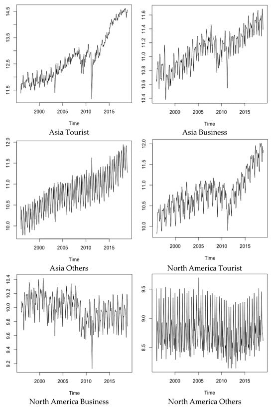
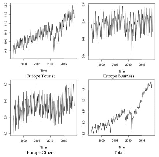
Figure 1.
Tourist arrivals in Japan disaggregated by three regions, purpose of travel, and the total (in log).
The summary statistics for the monthly percentage change of the tourist arrivals are also given in Table 1. Overall, arrivals in Japan have experienced a substantial growth of 0.84% per month over this period. In particular, tourist arrivals show an average increase of 1.2%, 0.58%, and 0.64% for Asia, North America, and Europe. Business and Other arrivals from Asia also show monthly growth averages of 0.31% and 0.56%, whereas stagnation or decline applies for North America and Europe. The sample standard deviations indicate substantially higher volatility for the Other arrivals. The third column in Table 1 reports the seasonal R2. This computed in a regression of the monthly changes of the arrival data against twelve-monthly dummy variables. Except for Tourist and Business arrivals from Asia, seasonality accounts for over 80% of the variations in these times series. Indeed, all the Other arrival time series have an R2 of more than 90%. A substantially different feature of seasonality from tourist arrivals from Asia reflects differences in distances and traditions in North America and Europe compared with Asia.
Applying the EEMD method, the data for arrivals were decomposed into 7 IMFs and a remainder. A representative graph of the Total is presented in Appendix A, while other decomposition results are available upon request from the authors. It can be seen that the data for arrivals are decomposed form high frequency to low frequency components and a remainder. The remainder is the lowest frequency component and displays the long-term trend in the arrivals. The monotonous increasing trend of the remainder indicates that the condition to terminate the IMFs decomposition is satisfied and no further decomposition is required.
4. Forecast Evaluation
Our main concern is the investigation of the forecast performance of the forecast combination method. It begins by employing the method of EEMD to decompose the arrivals time series from high to low frequencies at the first stage. In the second stage, ARIMA, NN, and SVM forecasting models were used to forecast each decomposed component separately and then combined them to obtain the combination forecast. The NN, SVM, and ARIMA models were fitted to the observations set aside for training purposes. Out-of-sample forecasts from the three models were then calculated and, subsequently, the combination forecasts were obtained for the remaining test data.
To assess and compare the forecasting performance of these models, the out-of-sample MSEs were computed, and the modified Diebold–Mariano test (Harvey et al., 1997) was applied on the out of sample forecast errors to test for the significant difference between the errors produced by the forecast combination method and the benchmark models. We also reported a summary table of Relative Root Mean Squared Errors (RRMSE) shown below.
where represents the k = 1, 3, 6, or 12 step ahead forecasts computed by the single model, NN, SVM, or ARIMA. represents the k = 1, 3, 6, or 12 step ahead forecast obtained by the forecast combination method which exploits EEMD. The RRMSE has been used in several forecasting studies such as Silva et al. (2019), Hassani et al. (2009), and Silva et al. (2017) and references therein.
Forecasting Results
In this study, the forecast results by the SVM, NN, and ARIMA models, for the combined high IMFs and combined low IMF components decomposed by the EEMD method, were subsequently used to obtain the final combination forecast. To investigate the forecasting performance of the combination method, the SVM, ARIMA, and NN models were then selected as the benchmark models for assessment. Table 2 presents the out-of-sample Mean Square Error (MSE) for 1, 3, 6, and 12-month forecasts of nine time series, categorized by continent and travel purpose. The EEMD model optimally combines forecasts of decomposed high- and low-frequency IMFs using different methods. The modified Diebold–Mariano test assesses the significance of differences between forecast errors of the benchmark EEMD model and other models.
Table 2.
Out-of-sample MSE for Asia, Europe and North America, and Total based on the purpose of travel.
We begin by analyzing the results for tourist arrivals from Asia. First and foremost, we notice that the NN model is the worst contender (in a majority of the instances) in comparison to the competing models across all horizons. Secondly, the combination forecast from the EEMD model outperforms all competing models across all horizons based on the MSE criterion. However, a closer look at the results shows that in the very short run (1-month ahead) and very long run (12-months ahead), there is no evidence of statistically significant differences between forecasts from the combination model and competing forecasts in terms of forecasting Asians arriving for tourism purposes. This indicates the findings on these horizons could be chance occurrences. The findings also show evidence for statistically significant differences in forecasts between the combination forecast and competing models at h = 1, 3, and 6 steps-ahead for arrivals relating to business and other purposes. In the very long run, the results are comparatively less convincing from a statistical significance perspective, but evidence indicates that the combination forecasts are significantly better than ARIMA forecasts for arrivals into Japan for business and other purposes at this horizon.
In the case of Europe, the performance of the forecast combination model at generating forecasts for tourist arrivals into Japan is significantly better than the competing models in the very short run. However, as the horizon increases, there is a considerable drop in statistically significant outcomes even though the forecast combination model continues to produce the lowest MSE in comparison to the competing models. Interestingly, the forecast combination model outperforms ARIMA significantly across all cases except for arrivals for tourism purposes at h = 12 months-ahead.
In terms of arrivals from North America, at horizons of 1, 3, and 6 months-ahead the combination forecasts are significantly better than the competing forecasts for tourism and business purpose arrivals into Japan. Interestingly, there is only one statistically significant case whereby the combination forecast is significantly better than a competing forecast when it comes to arrivals into Japan for other purposes. Nevertheless, based on the MSE it is evident that combination forecasts continue to outperform the other models in terms of reporting the lowest MSE across all cases at each forecasting horizon.
Table 2 also presents the out-of-sample MSE for 1, 3, 6, and 12-month forecasts of total inbound tourist arrivals to Japan. The EEMD model optimally combines forecasts of decomposed high- and low-frequency IMFs using different methods. At h = 1 and h = 3 steps-ahead, there are statistically significant differences between the combination forecasts and competing forecasts based on the modified Diebold–Mariano test. However, interestingly, in the very long run (at h = 12 steps-ahead) we do not find any evidence of statistically significant differences between the combination forecasts and others for the Total. Even at h = 6 steps-ahead, the combination forecasts do not outperform the ARIMA forecasts significantly. This indicates that there is more confidence in the capabilities of the combination forecasting model at generating more accurate forecasts for the Total at h = 1 or h = 3 steps-ahead as opposed to h = 12, or h = 6 steps-ahead (except in comparison to SVM and NN forecasts), as it is evident from Table 1 that data for the Total have the smallest volatility and show a linear long-term trend. Therefore, a linear model such as ARIMA can capture this pattern well and produce good long-term forecasts for this time series data.
Overall, as can be seen from Table 2, the forecast errors obtained by SVM and ARIMA models, in most cases, produced better results than the NN model. The prediction errors of the combined forecasting model are lower than that of the NN, SVM, and ARIMA models and proved to be statistically significantly better. The forecasting results suggest the superiority of the combined forecasting model when the forecast combination technique was used to decompose the original data. Table 3 displays the RRMSE, which is the ratio of the RMSE of the optimized EEMD combination forecast to the RMSE of individual Support Vector Machine, Neural Network, and ARIMA forecasts. The last column of Table 3 presents the average RRMSE for 1, 3, 6, and 12 steps ahead forecasts. The score indicates how many times out of 10 the EEMD model achieves a lower RMSE for each forecast horizon/method. The results show that, in terms of the average RRMSE, the improvement in the combined model compared with SVM, NN, and ARIMA can be of orders of 28%, 46%, and 19%, respectively. The second summary statistic in Table 3 is a score of the number of times out of 10 that the combination forecast yields lower MSE at the given horizon/method. In terms of different methods, the results show that the combination forecast outperforms SVM in 32 cases, NN for 39 cases, and ARIMA for 35 out of 40 times.
Table 3.
Out-of-Sample relative RMSE.
In terms of different horizons, the combination forecast outperformed other models by 25% for the one-month ahead forecasts. The dominance of the optimal forecasting model, applying the EMD technique, increases in longer term forecasts. The improvements are in the order of around 33% for the horizons of 3, 6, and 12 months ahead. The results also indicate that EEMD outperformed the other three methods in 24 cases out of 30 for one step ahead forecasts, and in 27 cases out of 30 for longer term forecasts. In addition, we report the Mean of Errors as a measure of Bias in Table 4, and the out of sample Mean Absolute Errors (MAE) were computed and are available from the authors upon request.
Table 4.
Out-of-sample Mean Errors.
Overall, the results indicate that the combination forecast outperformed the other three methods by 31% (based on the RRMSE). Compared with SVM, NN, and ARIMA, in 88% of cases (106/120) the combination forecast also produced a lower MSE. We also tested for the statistical significance of equality of the post-sample forecasting errors between the EEMD and the benchmark models at the horizons of 1, 3, 6, and 12 months ahead. The results indicate that in 62.5% (75/120) of cases, the forecast combination model is significantly better than the other methods at either 1% or 5% levels. Similarly, the results for out-of-sample Mean Absolute Errors (available from the authors upon request) for the 1, 3, 6, and 12 months ahead forecasts of the nine-time series, disaggregated based on the purpose of travel and the Total, show that, overall, the combination forecasts outperformed other models in 90% of cases, again confirming the superiority of the combination forecasting model applying the EEMD technique. Table 4 shows the mean of the out-of-sample forecast errors for EEMD, SVM, NN, and ARIMA. This serves as a measure of forecast bias in addition to the RMSE reported. Regarding the bias, the results in this table indicate that, in general, both ARIMA and combination forecasting models have produced much better forecasts than SVM and NN models at all horizons.
5. Discussions and Conclusions
Japan continues to progress into an important global tourist destination. Historically, research into improving the accuracy of tourism demand forecasts in Japan have been sparse, but given its growing importance, we find it pertinent to consider a forecast evaluation for Japanese tourism demand, to inform stakeholders on the suitability of a selection of forecasting methodologies. In this study, three components of arrivals, Tourist, Business, and Others, in Japan from Asia, North America, and Europe were considered. These time series data were decomposed by utilizing the EEMD approach. The combination models of SVM, NN, and ARIMA models were then used to predict the arrivals for ten time series, nine disaggregated time series, and the monthly Total arrivals to Japan.
We found that SVM and ARIMA models had produced much better forecasts than the non-linear NN models. The NN model demonstrated the worst performance in terms of forecasting Japanese tourism demand in majority of the cases considered here. When comparing the combined forecasting model with the benchmarks, the results proved the superiority of the combination forecasts over using only the single model for forecasting the tourism demand in Japan.
The results showed that the MSE of EEMD were smaller than other approaches in 88% of cases. In fact, on average, in terms of RRMSE, the combined models using EEMD outperformed SVM, NN, and ARIMA by 28%, 46%, and 19%. In terms of different horizons, EEMD outperformed other models by 25% for the one-month ahead forecasts. The dominance of the combined forecasts increases, for longer term horizons, and the gains are in the order of around 33% for the 3, 6, and 12 months ahead forecasts. Overall, the results indicated that EEMD outperformed the other three methods by 31% in terms RRMSE and in 106 out of 120 cases considered, using the three methods and for four different forecast horizons. Overall, this study shows that the forecast performance of the forecast combination model, using EEMD decomposition, is much better than the benchmark models and thus more suitable for predicting the tourism data.
Given that our conclusions support the superiority of the EEMD based forecast combination approach, we find it pertinent to discuss why this model is worthy of consideration in tourism forecasting contexts. Firstly, the IMFs partially reveal the characteristics of the data, with its remainder presenting the internal trend. The second advantage of the decomposition method by EEMD is its ability to deal with nonlinearity and nonstationarity without changing the original features of the data. This means that the forecasts obtained by the combination method can be directly compared with the original data. EMD is affected by modal aliasing. To overcome this problem, the EEMD approach was developed which avoids the aliasing produced via EMD by adding a series of pure noise to the original data. Another important feature of the EEMD method is that the added noise can effectively be cancelled, resulting in improvements in forecast accuracy (Fang et al., 2020). In addition, the superiority of the forecast combination employing EEMD decomposition becomes more pronounced as more individual models are included. Finally, EEMD-based forecast combination methods have been widely adopted as solutions to forecasting problems in different fields, thereby further confirming its value within our application (see, for example, Z. Zhang and Hong (2019) and Ali et al. (2020)).
Our findings can be of importance to the Japanese government and stakeholders like Japanese Tourism Research & Consulting Co. within the tourism industry. For example, the Japan National Tourism Organisation and Japanese Tourism Research & Consulting Co. can benefit by using this approach as a means of enhancing the tourism demand forecasting accuracy of its existing approaches. The ability to generate more accurate forecasts will directly feed into more efficient resource allocations and also aid in better planning and decision making within the tourism industry.
This paper opens up several avenues for future research. First, recent advancements in Japan’s status on the global tourism front confirms that there is a growing need for more applications in forecasting Japanese tourism demand. As such, researchers should consider developing more comparative studies evaluating forecasting accuracy across a broad range of forecasting models. Secondly, there is scope to evaluate more varied forecast combinations in the context of Japanese tourism demand. Researchers should not only consider comparing more varied univariate models with the forecast combinations suggested here, but also compare the performance of other forecast combinations against the results reported here. Thirdly, the application of more complex, yet potentially more accurate, multivariate forecasts should be considered as a viable option for generating further accuracy improvements in Japanese tourism demand forecasts. Fourthly, researchers can consider several other decomposition techniques such as wavelet transform, singular spectrum analysis, or independent component analysis in relation to EEMD to determine the most optimal decomposition for Japanese tourism demand. Furthermore, as COVID-19 has driven the e-commerce and digital initiatives across all business sectors, multivariate models could also consider search index data as a leading indicator for predicting global demand for Japan as a tourist destination. Finally, the forecasting performance of EEMD in disruptive data, such as during the COVID-19 pandemic, is an interesting topic we are currently investigating.
Author Contributions
Conceptualization, Y.F. and S.H.; methodology, Y.F.; software, Y.F.; validation, S.H., B.G., and H.H.; formal analysis, E.S.S. and S.H.; investigation, Y.F.; resources, Y.F.; data curation, B.G.; writing—original draft preparation, Y.F.; B.G., and E.S.S., writing—review and editing, S.H., H.H., and B.G.; visualization, Y.F.; supervision, S.H. and B.G.; project administration, B.G. and H.H.; funding acquisition, Y.F. All authors have read and agreed to the published version of the manuscript.
Funding
Guangdong Provincial Natural Science Foundation (Project Number: 2024A1515010941) and Guangdong Planning of Philosophy and Social Science (Project Number: GD23XYJ65).
Institutional Review Board Statement
Not applicable.
Informed Consent Statement
Not applicable.
Data Availability Statement
The data presented in this study were derived from the following resources available in the public domain: Japan National Tourism Organization (JNTO) [https://statistics.jnto.go.jp/en/graph/#graph--latest—figures, accessed on 26 April 2025]. The raw data supporting the conclusions of this article will be made available by the authors on request.
Acknowledgments
The authors would like to thank the anonymous reviewers and editor for their constructive feedback and suggestions.
Conflicts of Interest
The authors declare no conflicts of interest.
Appendix A
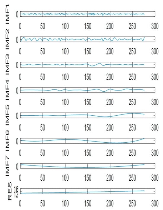
Figure A1.
IMFs of Arrivals (IMFs) after EEMD decomposition for Japanese inbound tourist arrivals in aggregate Total.
References
- Ali, M., Prasad, R., Xiang, Y., & Yaseen, Z. M. (2020). Complete ensemble empirical mode decomposition hybridized with random forest and kernel ridge regression model for monthly rainfall forecasts. Journal of Hydrology, 584, 124–647. [Google Scholar] [CrossRef]
- Andonian, A., Kuwabara, T., Yamakawa, N., & Ishida, R. (2016). The future of Japan’s tourism: Path for sustainable growth towards 2020. McKinsey Japan and Travel, Transport and Logistics Practice. Retrieved February, 10, 2018. [Google Scholar]
- Atiya, A. F. (2020). Why does forecast combination work so well? International Journal of Forecasting, 36(1), 197–200. [Google Scholar] [CrossRef]
- Bekiroglu, K., Gulay, E., & Duru, O. (2022). A multi-method forecasting algorithm: Linear unbiased estimation of combine forecast. Knowledge-Based Systems, 239, 107990. [Google Scholar] [CrossRef]
- Bosupeng, M. (2019). Forecasting tourism demand: The Hamilton filter. Annals of Tourism Research, 79(C), 102823. [Google Scholar] [CrossRef]
- Chen, C. F., Lai, M. C., & Yeh, C. C. (2012). Forecasting tourism demand based on empirical mode decomposition and neural network. Knowledge-Based Systems, 26, 281–287. [Google Scholar] [CrossRef]
- Chen, W., Sun, J., Gao, S., Cheng, J. J., Wang, J., & Todo, Y. (2017). Using a single dendritic neuron to forecast tourist arrivals to Japan. IEICE Transactions on Information and Systems, 100(1), 190–202. [Google Scholar] [CrossRef]
- Fang, Y., Guan, B., Wu, S., & Heravi, S. (2020). Optimal forecast combination based on ensemble empirical mode decomposition for agricultural commodity futures prices. Journal of Forecasting, 39(6), 877–886. [Google Scholar] [CrossRef]
- Fritz, R. G., Brandon, C., & Xander, J. (1984). Combining time-series and econometric forecast of tourism activity. Annals of Tourism Research, 11(2), 219–229. [Google Scholar] [CrossRef]
- Gunter, U., Önder, I., & Smeral, E. (2020). Are combined tourism forecasts better at minimizing forecasting errors? Forecasting, 2(3), 211–229. [Google Scholar] [CrossRef]
- Harvey, D., Leybourne, S., & Newbold, P. (1997). Testing the equality of prediction mean squared errors. International Journal of Forecasting, 13(2), 281–291. [Google Scholar] [CrossRef]
- Hassani, H., Heravi, S., & Zhigljavsky, A. (2009). Forecasting European industrial production with singular spectrum analysis. International Journal of Forecasting, 25(1), 103–118. [Google Scholar] [CrossRef]
- Hassani, H., Webster, A., Silva, E. S., & Heravi, S. (2015). Forecasting US tourist arrivals using optimal singular spectrum analysis. Tourism Management, 46, 322–335. [Google Scholar] [CrossRef]
- Heravi, S., Osborn, D. R., & Birchenhall, C. R. (2004). Linear versus neural network forecasts for European industrial production series. International Journal of Forecasting, 20(3), 435–446. [Google Scholar] [CrossRef]
- Huang, N. E., Shen, Z., Long, S. R., Wu, M. C., Shih, H. H., Zheng, Q., Yen, N. C., Tung, C. C., & Liu, H. H. (1998). The empirical mode decomposition and the Hilbert spectrum for nonlinear and non-stationary time series analysis. Proceedings of the Royal Society of London. Series A: Mathematical, Physical and Engineering Sciences, 454(1971), 903–995. [Google Scholar] [CrossRef]
- Jiao, E. X., & Chen, J. L. (2019). Tourism forecasting: A review of methodological developments over the last decade. Tourism Economics, 25(3), 469–492. [Google Scholar] [CrossRef]
- Kourentzes, N., Saayman, A., Jean-Pierre, P., Provenzano, D., Sahli, M., Seetaram, N., & Volo, S. (2021). Visitor arrivals forecasts amid COVID-19: A perspective from the Africa team. Annals of Tourism Research, 88, 103197. [Google Scholar] [CrossRef] [PubMed]
- Kummong, R., & Supratid, S. (2016). Thailand tourism forecasting based on a hybrid of discrete wavelet decomposition and NARX neural network. Industrial Management & Data Systems, 116(6), 1242–1258. [Google Scholar]
- Lai, M. C., Yeh, C. C., & Shieh, L. F. (2013). A hybrid model by empirical mode decomposition and support vector regression for tourist arrivals forecasting. Journal of Testing and Evaluation, 41(3), 351–358. [Google Scholar] [CrossRef]
- Law, R. (2001). The impact of the Asian financial crisis on Japanese demand for travel to Hong Kong: A study of various forecasting techniques. Journal of Travel & Tourism Marketing, 10(2–3), 47–65. [Google Scholar]
- Li, G., Wu, D. C., Zhou, M., & Liu, A. (2019). The combination of interval forecasts in tourism. Annals of Tourism Research, 75, 363–378. [Google Scholar] [CrossRef]
- Li, X., & Law, R. (2020). Forecasting tourism demand with decomposed search cycles. Journal of Travel Research, 59(1), 52–68. [Google Scholar] [CrossRef]
- Liu, A., Vici, L., Ramos, V., Giannoni, S., & Blake, A. (2021). Visitor arrivals forecasts amid COVID-19: A perspective from the Europe team. Annals of Tourism Research, 88, 103182. [Google Scholar] [CrossRef]
- Pai, P. F., Hong, W. C., Chang, P. T., & Chen, C. T. (2006). The application of support vector machines to forecast tourist arrivals in Barbados: An empirical study. International Journal of Management, 23(2), 375–385. [Google Scholar]
- Park, S., Lee, J., & Song, W. (2017). Short-term forecasting of Japanese tourist inflow to South Korea using Google trends data. Journal of Travel & Tourism Marketing, 34(3), 357–368. [Google Scholar]
- Polunin, I. (1989). Japanese travel boom. Tourism Management, 10(1), 4–8. [Google Scholar] [CrossRef]
- Russell, L. (2017). Assessing Japan’s inbound tourism: A SWOT analysis. Hannami Theory Social Science, 53(1), 21–50. [Google Scholar]
- Silva, E. S., Ghodsi, Z., Ghodsi, M., Heravi, S., & Hassani, H. (2017). Cross country relations in European tourist arrivals. Annals of Tourism Research, 63, 151–168. [Google Scholar] [CrossRef]
- Silva, E. S., Hassani, H., Heravi, S., & Huang, X. (2019). Forecasting tourism demand with denoised neural networks. Annals of Tourism Research, 74, 134–154. [Google Scholar] [CrossRef]
- Song, H., Qiu, R. T., & Park, J. (2019). A review of research on tourism demand forecasting: Launching the Annals of Tourism Research Curated Collection on tourism demand forecasting. Annals of Tourism Research, 75, 338–362. [Google Scholar] [CrossRef]
- Song, H., Witt, S. F., & Li, G. (2003). Modelling and forecasting the demand for Thai tourism. Tourism Economics, 9(4), 363–387. [Google Scholar] [CrossRef]
- Soshiroda, A. (2005). Inbound tourism policies in Japan from 1859 to 2003. Annals of Tourism Research, 32(4), 1100–1120. [Google Scholar] [CrossRef]
- Sun, Y., Zhang, J., Li, X., & Wang, S. (2021). Forecasting tourism demand with a new time-varying forecast averaging approach. Journal of Travel Research, 62(2), 305–323. [Google Scholar] [CrossRef]
- Tang, L. H., Bai, Y. L., Yang, J., & Lu, Y. N. (2020). A hybrid prediction method based on empirical mode decomposition and multiple model fusion for chaotic time series. Chaos, Solitons & Fractals, 141, 110366. [Google Scholar]
- Turner, L. W., Kulendran, N., & Fernando, H. (1997). Univariate modelling using periodic and non-periodic analysis: Inbound tourism to Japan, Australia and New Zealand compared. Tourism Economics, 3(1), 39–56. [Google Scholar] [CrossRef]
- UNWTO. (2019). International tourism highlights: 2019 edition. Available online: https://www.e-unwto.org/doi/pdf/10.18111/9789284421152 (accessed on 10 May 2024).
- UNWTO. (2024). International tourist arrivals hit 96% of pre-pandemic levels through July 2024. Available online: https://www.unwto.org/news/international-tourist-arrivals-hit-96-of-pre-pandemic-levels-through-july-2024 (accessed on 10 May 2024).
- Vapnik, V. (1998). Statistical learning theory new york. Wiley. [Google Scholar]
- Wong, K. K., Song, H., Witt, S. F., & Wu, D. C. (2007). Tourism forecasting: To combine or not to combine? Tourism Management, 28(4), 1068–1078. [Google Scholar] [CrossRef]
- Wu, J., Cheng, X., & Liao, S. S. (2020). Tourism forecast combination using the stochastic frontier analysis technique. Tourism Economics, 26(7), 1086–1107. [Google Scholar] [CrossRef]
- Wu, Z., & Huang, N. E. (2009). Ensemble empirical mode decomposition: A noise-assisted data analysis method. Advances in Adaptive Data Analysis, 1(01), 1–41. [Google Scholar] [CrossRef]
- Xie, G., Qian, Y., & Wang, S. (2020). A decomposition-ensemble approach for tourism forecasting. Annals of Tourism Research, 81, 102891. [Google Scholar] [CrossRef]
- Xu, X., Law, R., Chen, W., & Tang, L. (2016). Forecasting tourism demand by extracting fuzzy Takagi-Sugeno rules from trained SVMs. CAAI Transactions on Intelligence Technology, 1(1), 30–42. [Google Scholar] [CrossRef]
- Yagasaki, N. (2021). Impact of COVID-19 on the Japanese travel market and the travel market of overseas visitors to Japan, and subsequent recovery. IATTS Research, 45, 451–458. [Google Scholar] [CrossRef]
- Yahya, N. A., Samsudin, R., & Shabri, A. (2017). Tourism forecasting using hybrid modified empirical mode decomposition and neural network. International Journal of Advances in Soft Computing and Its Applications, 9(1), 14–31. [Google Scholar]
- Yeh, J. R., Shieh, J. S., & Huang, N. E. (2010a). Complementary ensemble empirical mode decomposition: A novel noise enhanced data analysis method. Advances in Adaptive Data Analysis, 2(02), 135–156. [Google Scholar] [CrossRef]
- Yeh, J. R., Sun, W. Z., Shieh, J. S., & Huang, N. E. (2010b). Investigating fractal property and respiratory modulation of human heartbeat time series using empirical mode decomposition. Medical Engineering & Physics, 32(5), 490–496. [Google Scholar]
- Zhang, G., Wu, J., Pan, B., Li, J., Ma, M., Zhang, M., & Wang, J. (2017). Improving daily occupancy forecasting accuracy for hotels based on EEMD-ARIMA model. Tourism Economics, 23(7), 1496–1514. [Google Scholar] [CrossRef]
- Zhang, Y., Li, G., Muskat, B., & Law, R. (2021). Tourism demand forecasting: A decomposed deep learning approach. Journal of Travel Research, 60(5), 981–997. [Google Scholar] [CrossRef]
- Zhang, Z., & Hong, W. C. (2019). Electric load forecasting by complete ensemble empirical mode decomposition adaptive noise and support vector regression with quantum-based dragonfly algorithm. Nonlinear Dynamics, 98(2), 1107–1136. [Google Scholar] [CrossRef]
Disclaimer/Publisher’s Note: The statements, opinions and data contained in all publications are solely those of the individual author(s) and contributor(s) and not of MDPI and/or the editor(s). MDPI and/or the editor(s) disclaim responsibility for any injury to people or property resulting from any ideas, methods, instructions or products referred to in the content. |
© 2025 by the authors. Licensee MDPI, Basel, Switzerland. This article is an open access article distributed under the terms and conditions of the Creative Commons Attribution (CC BY) license (https://creativecommons.org/licenses/by/4.0/).