Machine Learning-Based Estimation of Daily Reference Evapotranspiration in Vojvodina, Serbia

Abstract

Reference evapotranspiration (ET₀) is most commonly estimated using the FAO-56 Penman–Monteith (PM) equation. However, its application is often limited by the lack of required meteorological parameters. Due to their flexibility, ability to operate with limited input, and high accuracy in estimating ET₀, machine learning models have become increasingly relevant in scientific research, offering a practical alternative under limited data conditions. In this study, artificial neural networks (ANNs) were applied to estimate daily ET₀ using meteorological data from the Novi Sad station in Vojvodina (Serbia). The dataset consisted of eight meteorological variables relevant to evapotranspiration processes. Analysis showed that some variables had a stronger influence on ET₀ prediction than others. To evaluate their combined effect, a series of ANN models with different input combinations were developed and tested. The random forests, gradient boosting and k-nearest neighbors models were used as a benchmark, and model performance was evaluated using R², NSE, RMSE, and MAE. The highest accuracy was achieved when all variables were included, providing the model with maximum information. The best performance was obtained using a two-hidden-layer architecture with 32 and 16 neurons, resulting in R² = 0.97, NSE = 97.07%, RMSE = 0.23 mm/day, and MAE = 0.21 mm/day. The results showed that a limited number of input variables can be used to estimate ET₀ with high accuracy, achieving an R² value of 0.95 using only three input variables. Therefore, the findings of this study may contribute to more accurate and cost-effective irrigation scheduling and water balance estimation, providing practical benefits for agricultural water management and farmers in Serbia.

1. Introduction

Evapotranspiration (ET) is a key component of the hydrologic cycle, as it governs the transfer of moisture to the atmosphere and affects vital features of terrestrial ecosystems, such as runoff, soil moisture, and plant growth, which are critical to water availability [1,2,3,4,5]. ET is a complex process because it depends on the interactions among atmospheric, soil, and plant parameters [6]. Due to this complexity, it is essential in various fields of research, including the optimization of water resource use, crop yield simulation, irrigation and management system design, hydrological balance assessment, and improving water use efficiency in agriculture [7,8,9]. Accurate ET estimation is crucial for efficient irrigation management [10]. Reference evapotranspiration (ET₀) is a climatic parameter that represents the atmospheric demand for evaporation from a reference surface. The reference surface is a hypothetical grass crop with a height of 0.12 m, a fixed surface resistance of 70 s m⁻¹, and an albedo of 0.23 [11]. Accurate estimation of ET₀ is essential for simulating the global water cycle and for making irrigation decisions [12,13,14,15,16]. ET₀ can be determined through direct measurements, such as the use of lysimeters, which are accurate but demanding in terms of time, cost, and resources. Therefore, empirical methods are most commonly used in practice, with the FAO-56 Penman–Monteith (FAO-56 PM) equation being considered the most reliable.

According to the Food and Agriculture Organization of the United Nations (FAO), the standard method for calculating ET₀ is the FAO-56 PM equation, which has proven to be the most reliable under different climatic conditions [17,18,19,20]. The method represents a parameterized adaptation of the original Penman–Monteith model [21], which is a widely used physical model for estimating actual evapotranspiration. However, to calculate ET₀ using the FAO-56 PM method, numerous meteorological parameters are required, which limits its application in regions lacking complete input data [22,23,24,25,26]. In addition to the FAO-56 PM method, alternative approaches have been considered for calculating ET₀ in situations with a limited number of input parameters. One approach is the replacement of the FAO-56 PM equation with a simplified empirical formula, while another is the use of machine learning techniques to directly simulate ET₀ based on a reduced input set, which is the main focus of this study.

Machine learning (ML) is a technique within the field of artificial intelligence that relies on the idea that systems can learn from data, identify patterns, and make decisions with minimal human involvement [27]. ML techniques are applied in situations involving large datasets and numerous variables that change over time, particularly in domains where the use of predefined formulas or equations is difficult. ML models can be applied to predict daily ET based on extensive climatic datasets, even in the absence of detailed knowledge about the physical ET process. The application of ML techniques, particularly artificial neural networks, in modeling hydrological processes such as ET has attracted significant attention from researchers [28,29,30,31,32,33,34,35]. In this study we used three popular and in practice proven ML models: random forests, gradient boosting and k-nearest neighbors’ models. These models were used as a benchmark for performance of neural network.

Artificial neural networks (ANNs) are algorithmic structures inspired by the functioning of the biological nervous system in the human brain [36,37]. ANN is frequently used for modeling ET due to its ability to recognize and reproduce complex input–output relationships without the need for detailed knowledge of the physical process [6]. Due to their flexible nature, neural networks enable the development of models without requiring prior knowledge of data distribution or interactions among variables, which is often necessary in parametric statistical methods [38].

Mallikarjuna et al. [39] investigated the applicability of linear regression and ANN models for estimating ET₀. They identified air temperature, wind speed, relative humidity, and sunshine hours as the most influential climatic variables. The optimal ANN models consistently demonstrated better performance than regression models in estimating daily ET₀. Dimitriadou and Nikolakopoulos [40] examined the use of ANN for estimating ET₀ during winter and summer months. Their study aimed to evaluate whether a reduced number of input parameters could yield satisfactory ET₀ predictions. Makwana et al. [41] examined the effectiveness of the ANN in estimating ET₀ using a limited number of meteorological input parameters. Their results showed that ANN models trained with all five input variables (maximum and minimum temperature, relative humidity, wind speed, and bright sunshine hours) achieved high accuracy, while variations in input combinations and network architecture significantly affected model performance. Naresh et al. [42] evaluated the performance of ANN models for estimating ET₀ using long-term meteorological data. Their results showed that the best performance was achieved with a single hidden layer of thirteen neurons trained using the Levenberg–Marquardt algorithm. El-Magd et al. [43] developed and tested seven ANN models using different combinations of five meteorological input parameters (maximum and minimum air temperature, dew point temperature, wind speed, and precipitation) to evaluate the accuracy of the ANN in estimating ET₀. The results indicated that ANN models provided accurate estimations, particularly when the temperature-related inputs were included, while precipitation had the least influence on prediction performance. Makwana et al. [44] evaluated the performance of several AI models, including the ANN, Extreme Learning Machine (ELM), M5 Tree, and Multiple Linear Regression (MLR), for estimating ET₀. The results showed that ANN models outperformed ELM, M5 Tree, and MLR in terms of various performance indicators when compared to the FAO-56 PM equation. Kumar et al. [45] used ANN models to simulate ET₀ at three meteorological stations. Different combinations of input parameters were tested and compared against the FAO-56 PM method. The best performance was achieved when all input parameters were included, while the lowest accuracy was observed when only air temperature and relative humidity were used. Skhiri et al. [46] estimated monthly ET₀ using ANN models based on meteorological data from multiple stations in Tunisia. Their study identified maximum air temperature as the most significant meteorological parameter influencing model accuracy.

Based on previous research, this study aims to evaluate the effectiveness of ANN models in estimating ET₀ under conditions of limited availability of meteorological data, through comparison with the standard FAO-56 PM method.

2. Materials and Methods

2.1. Study Area and Data Used

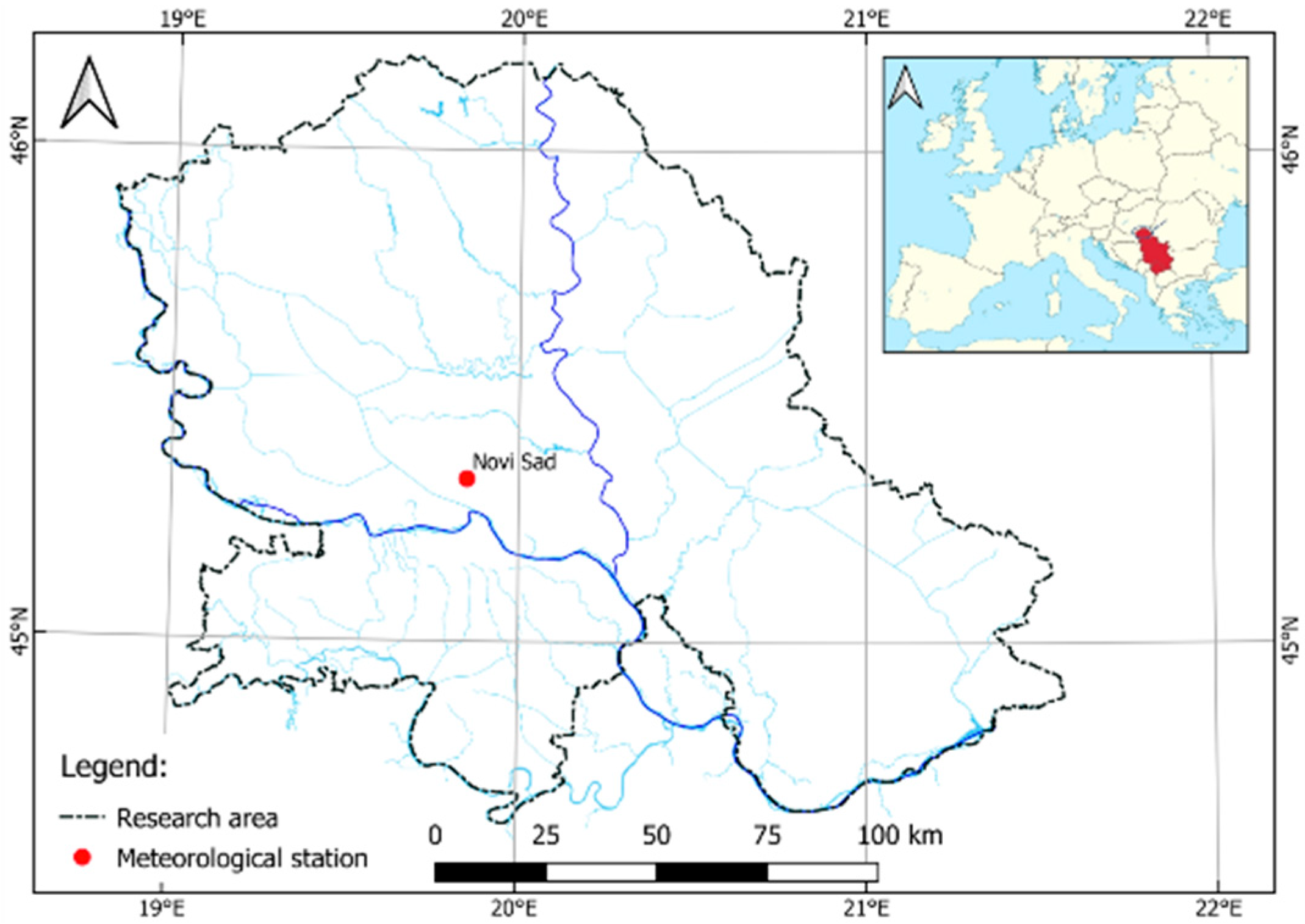
The Novi Sad meteorological station, located in the region of Vojvodina (Serbia), was selected in this study for ET₀ modeling using a limited set of meteorological parameters. The study area is located at latitude 45.33 °N and longitude 19.85 °E, with an elevation of 84 m above mean sea level (Figure 1). Based on its geographical location, the region is classified as having a temperate continental climate. Vojvodina is characterized by an extensive network of natural watercourses and canals that are part of the Danube–Tisa–Danube hydrosystem. The region is predominantly agricultural, with more than 17,500 km² of arable land, representing approximately 75% of its total area. In this study, daily meteorological data were used, including maximum, minimum, and mean air temperature (T_max, T_min, T_mean), relative humidity (RH), wind speed (WS), global radiation (GR), precipitation (P), and mean sea level pressure (SLP), covering the period from 1950 to June 2023. The data were obtained from the Copernicus Climate Change Service (C3S) [47].

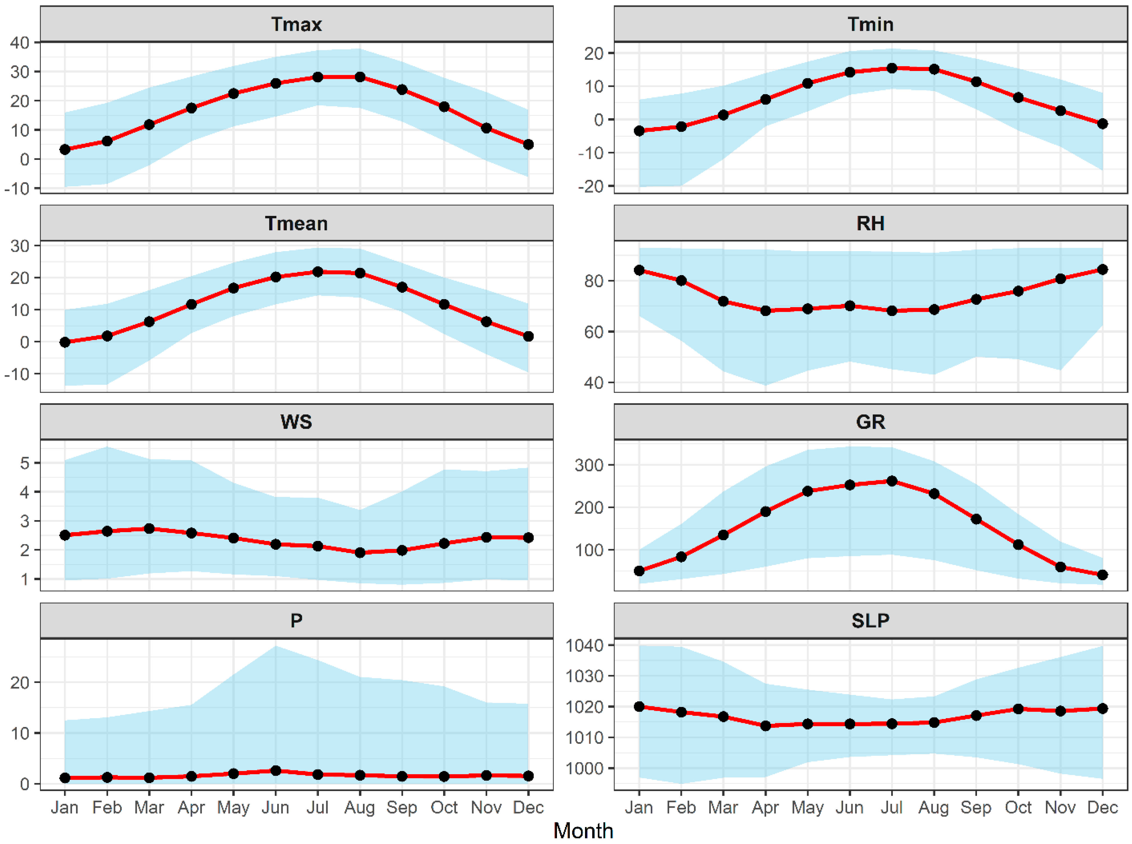
Maximum, minimum, and mean air temperature, relative humidity, wind speed, global radiation, precipitation, and mean sea level pressure ranged from −16.3 °C to 41.2 °C, −29.9 °C to 25.1 °C, −22.4 °C to 32.7 °C, 21.0% to 94.0%, 0.5 to 7.3 m s⁻¹, 0.1 W m⁻² to 470 W m⁻², 0 mm to 72.4 mm, and 976.6 hPa to 1046.2 hPa, respectively (

Table 1. Descriptive statistics of the available meteorological variables at the Novi Sad station.

Parameters	Tmax (°C)	Tmin (°C)	Tmean (°C)	RH (%)	WS (m s−1)	GR (W m−2)	P (mm)	SLP (hPa)
Xmin	−16.3	−29.9	−22.4	21.0	0.5	0.1	0	976.6
Xmax	41.2	25.1	32.7	94.0	7.3	470.0	72.4	1046.2
Xmean	16.8	6.4	11.4	74.4	2.3	152.6	1.6	1016.7
SX	10.2	7.8	8.8	11.7	0.8	93.3	4.0	7.6
CV	0.6	1.2	0.8	0.2	0.3	0.6	2.5	0.1
CSX	−0.3	−0.4	−0.2	−0.5	1.0	0.3	4.7	0.2

X_min = minimum value, X_max = maximum value, X_mean = mean value, S_X = standard deviation, C_V = coefficient of variation, C_SX = skewness coefficient.

). Mean values of the meteorological variables at the Novi Sad station for the period from 1950 to June 2023 are presented in Figure 2.

Mean values of the meteorological variables, as presented in Figure 2, exhibit a pronounced seasonal pattern typical for the observed region, with certain deviations. T_max, T_min, T_mean, and GR reach their peak during the summer months, while RH shows an inverse trend, increasing the potential for high ET₀. WS reaches its maximum in March and April and then declines during the summer period, whereas P records a peak in May and June, followed by a decrease in July and August, posing a risk of water deficit during the phase of highest crop water demand. By contrast, SLP displays an atypical seasonal pattern, with a maximum in January and a minimum in April, deviating from expected trends and indicating regional specificities in air mass circulation.

2.2. Estimation of Reference Evapotranspiration (ET₀)

The FAO Penman–Monteith method is widely recognized as the standard approach for calculating ET₀ based on meteorological data. It is recommended by the FAO [11]. This method combines energy balance and aerodynamic components, incorporating two resistance terms—surface and aerodynamic. Such a formulation provides highly accurate results, as it is grounded in physical principles and rational relationships [48]. In this study, the FAO-56 PM equation for estimating ET₀ is given by Allen et al. [11] as follows:

$${ ET}_0= {\displaystyle \frac{0.408 \Delta \left(R_n- G\right)+ \frac{900}{T+273} u_2(e_s-e_a)}{\Delta + \gamma (1+0.34u_2)}}$$

(1)

where ET₀ = reference evapotranspiration (mm/day), R_n = net radiation (MJ m⁻² day⁻¹), G = soil heat flux density (MJ m⁻² day⁻¹), T = mean daily air temperature at 2 m height (°C), u₂ = wind speed at 2 m height (m s⁻¹), e_s = saturation vapor pressure (kPa), e_a = actual vapor pressure (kPa), (e_s − e_a) = saturation vapor pressure deficit (kPa), Δ = slope of the vapor pressure curve (kPa °C⁻¹), and γ = psychrometric constant (kPa °C⁻¹).

2.3. Artificial Neural Networks (ANNs)

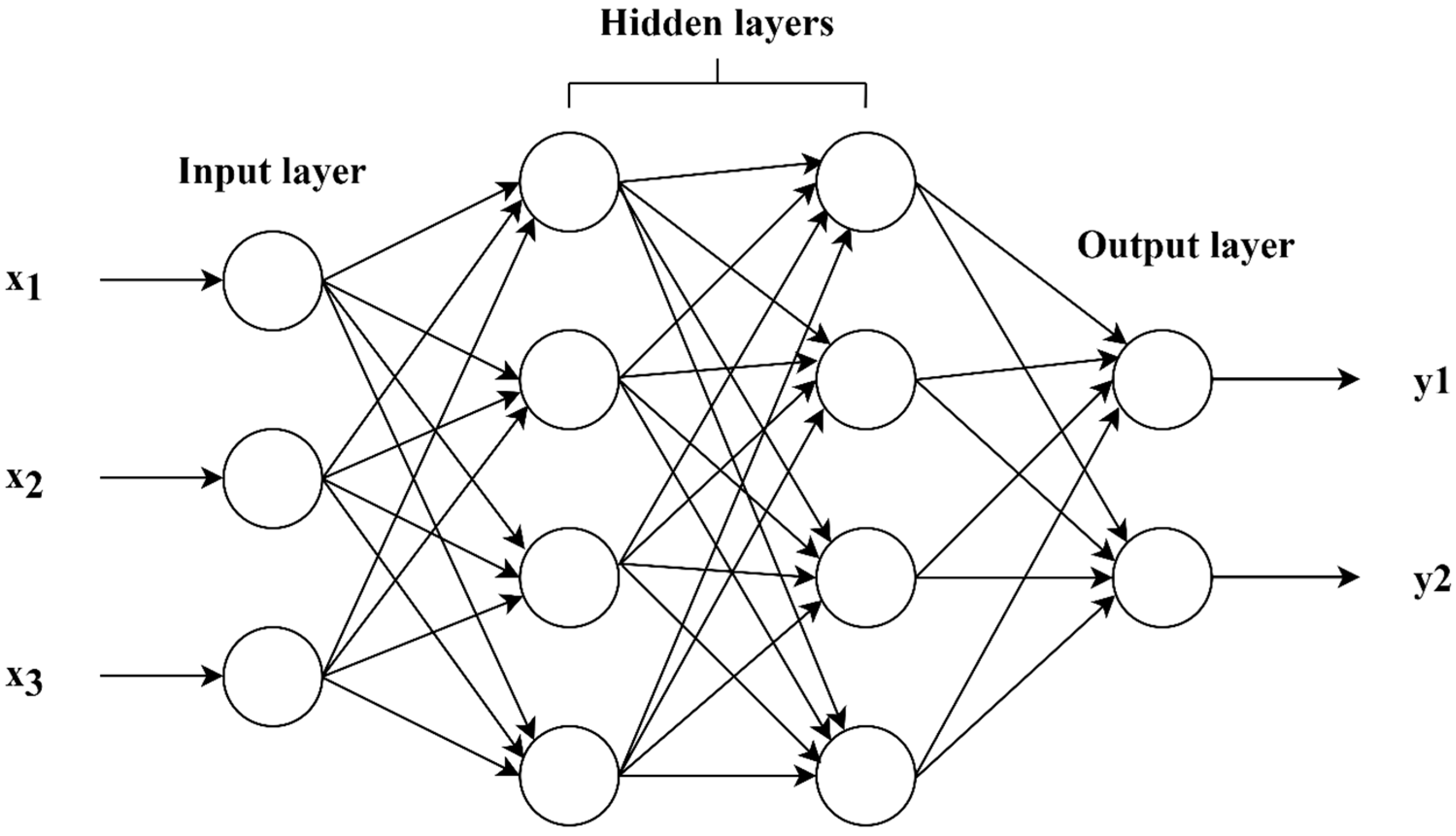
ANNs represent a form of nonlinear regression model that performs input–output mapping using a set of coefficients or weights [41,44]. ANNs are among the primary tools used in ML for pattern recognition, prediction, and forecasting [49], and have been successfully applied in various fields of scientific research. They consist of a network of processing units called neurons, which work collaboratively to solve specific problems. Typically, ANNs consist of input and output variables, along with one or more hidden layers (Figure 3). Each layer is fully connected to the subsequent layer through interconnection weights. These weights are initially assigned randomly and then adjusted during the training process [6]. The neural network layers contain multiple nodes and are structured as follows: (i) an input layer for introducing data into the system, (ii) one or more hidden layers for data processing during learning, and (iii) an output layer for generating predictions and decisions [50].

2.4. Performance Evaluation Criteria

The performance of the ANN models developed in this study was evaluated by comparing them with the reference FAO-56 PM method using standard statistical indicators, including the coefficient of determination (R²), Nash–Sutcliffe efficiency (NSE), root mean square error (RMSE), and mean absolute error (MAE) (

Table 2. Model performance evaluation metrics.

No.	Performance Criteria	Equation	Acceptable Range
1	Coefficient of determination (R2)	$R^2={\displaystyle \frac{[{\sum }_{i=1}^n(X_i-\underset{\_}{X})(Y_i-\underset{\_}{Y}){]}^2}{{\sum }_{i=1}^n(X_i-\underset{\_}{X}{)}^2{\sum }_{i=1}^n(Y_i-\underset{\_}{Y}{)}^2}}$	0 to 1
2	Nash–Sutcliffe efficiency (NSE)	$NSE=1-{\displaystyle \frac{{\sum }_{i=1}^n{\left(Y_i-X_i\right)}^2}{{\sum }_{i=1}^n{\left(X_i-\underset{\_}{X}\right)}^2}}$	0 to 100
3	Root mean square error (RMSE)	$RMSE=\sqrt{{\displaystyle \frac{1}{n}}{\displaystyle \sum _{i=1}^n}{\left(Y_i-X_i\right)}^2}$	>0
4	Mean absolute error (MAE)	$MAE={\displaystyle \frac{1}{n}}{\displaystyle \sum _{i=1}^n}\left|Y_i-X_i\right|$	>0

where $n$ is the number of observations, $X_i$ is the observed ET₀ value, $Y_i$ is the estimated ET₀ value, $\underset{\_}{X}$ is the mean of the observed ET₀ values, and $\underset{\_}{Y}$ is the mean of the estimated ET₀ values.

), to assess their accuracy and reliability. The model performance evaluation metrics and corresponding equations presented in Table 2 were adapted from previous studies [42,46].

3. Results and Discussion

3.1. FAO-56 PM Method

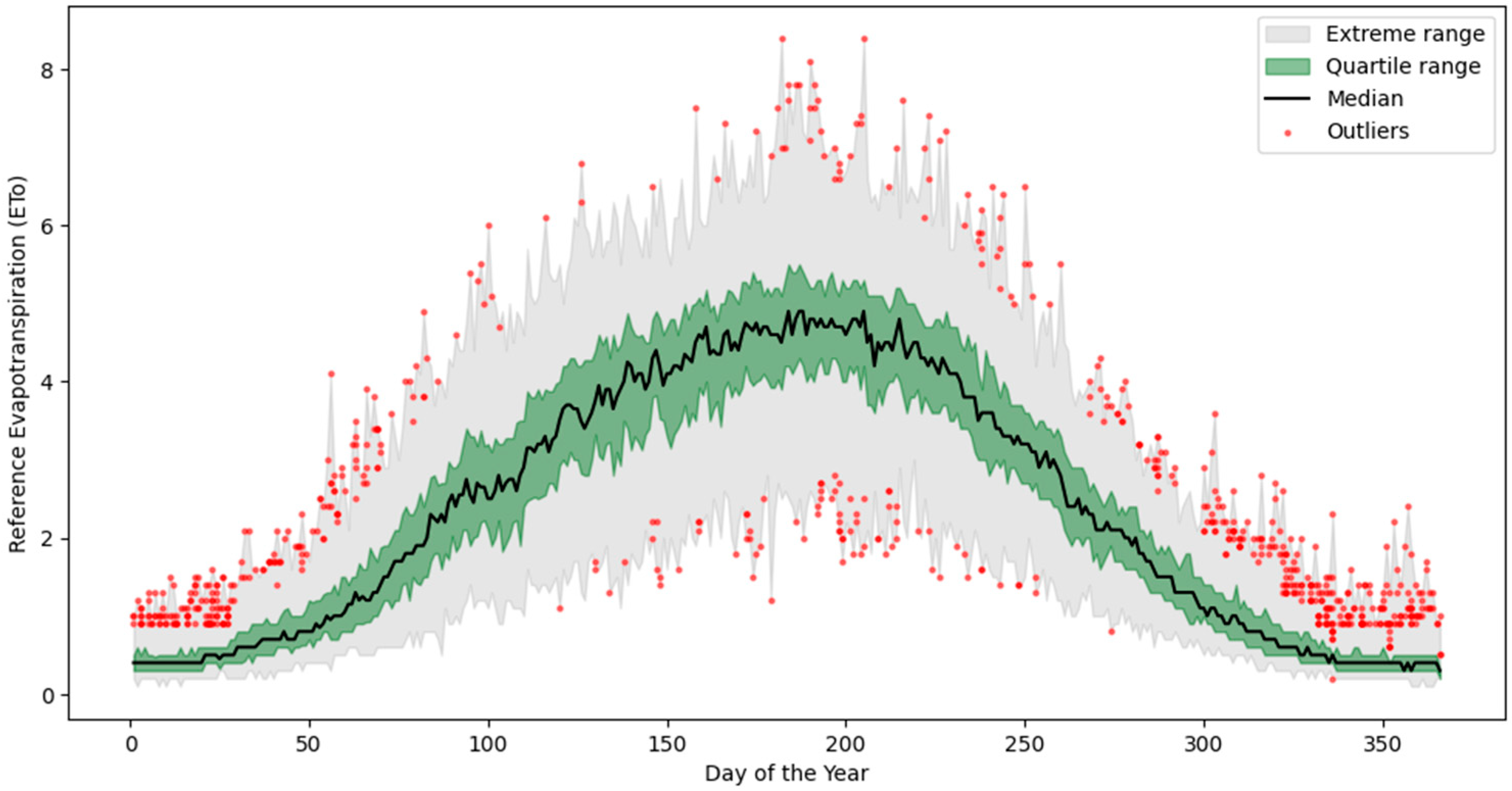
Daily ET₀ values were calculated for the period from 1950 to June 2023 using the FAO-56 PM method. Figure 4 illustrates the average daily ET₀ values over this period. ET₀ remained low during the winter months and progressively increased during spring, reaching its peak in July with a maximum of 8.4 mm/day. This seasonal trend is consistent with increased solar radiation, temperature, and wind speed during the summer.

The interquartile range indicates the spread of the middle 50% of the data, while the extreme range displays the minimum and maximum values recorded for each day. A higher number of outliers is observed during the summer months, likely resulting from interannual climatic variability and occasional extreme weather events.

These findings align with the expected seasonal dynamics of ET in temperate continental climates and underline the influence of meteorological factors such as temperature, radiation, and wind on daily ET₀ values.

3.2. Performance of ANN Models

The ANN model was developed using different combinations of input variables. For the period from 1950 to June 2023, the data were temporally divided into training, testing, and validation sets, with 70% of the first data used for training, 10% for model validation, and 20% for testing.

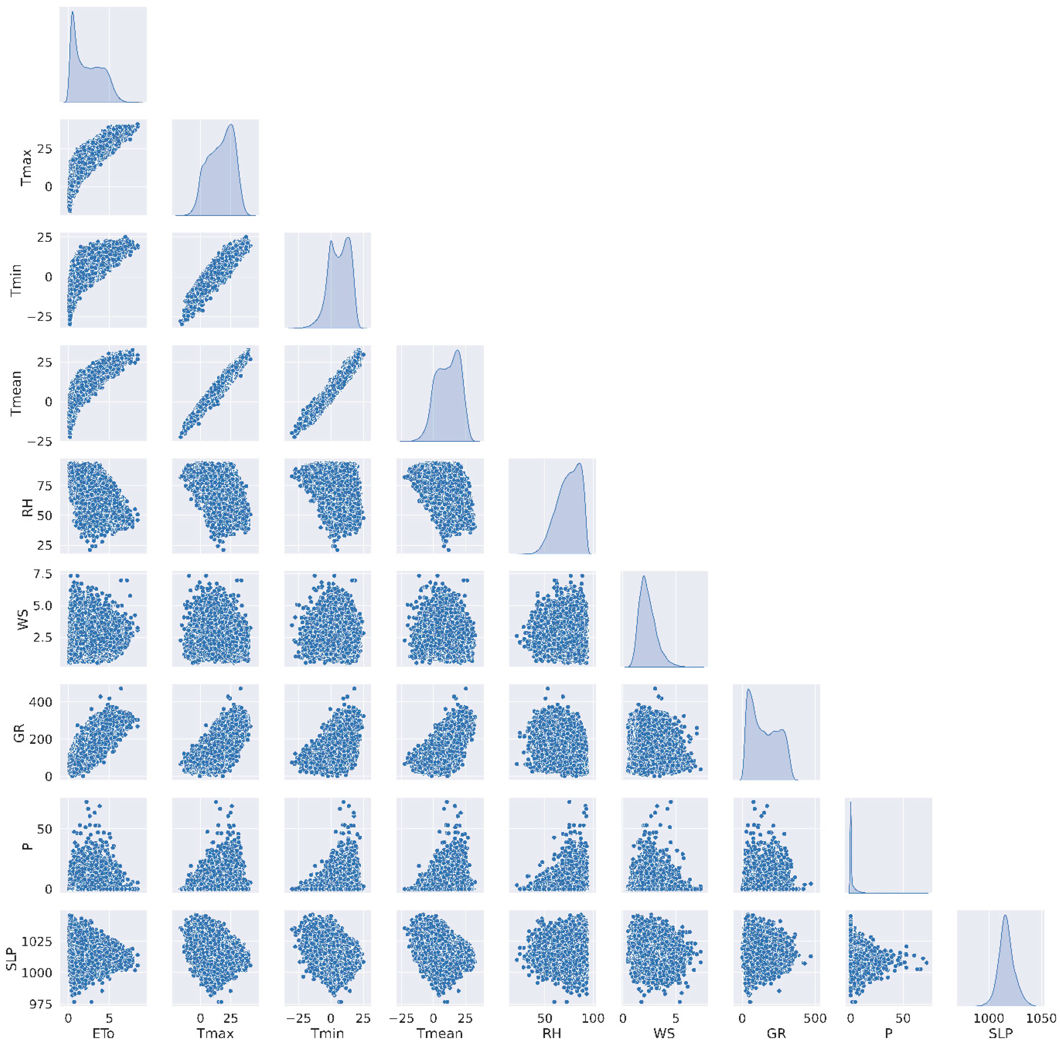
To examine the relationships between the meteorological variables used as model inputs, a pairwise scatterplot matrix (pairplot) was created (Figure 5). This visualization allows for the identification of potential linear and nonlinear dependencies between variables and provides an overview of their distributions. Strong linear correlation relationships are particularly evident among temperature-related parameters (T_max, T_min, T_mean), while other variables, such as WS, GR, P, and SLP, exhibit more scattered patterns.

The model begins with an input layer in which all input variables are normalized to enhance learning efficiency. Normalization was performed to scale the input variables to a range between 0 and 1. The ANN model consists of hidden layers, each containing a specific number of neurons. The hyperbolic tangent (tanh) activation function was used in the hidden layers due to its ability to model nonlinear patterns in the data. The output layer consists of a single neuron that predicts the normalized ET₀ values, with a linear activation function. For model training, the mean square error (MSE) was used as the loss function, while model optimization was performed using the Adam algorithm with default parameters and a learning rate of 1 × 10⁻⁴. Additionally, L2 regularization was applied to each hidden layer with a regularization coefficient of 4 × 10⁻⁵, whereas a reduced regularization value (1 × 10⁻⁸) was applied to the final linear output layer. This approach contributes to improved model generalization. The training was conducted using a batch size of 1024, while validation results were evaluated every 10th or 50th epoch to accelerate the training process without compromising accuracy. This approach enabled faster model training while maintaining a high level of predictive performance and generalization. The number of trainable parameters for the proposed ANN architecture is 6391 trainable parameters.

The performance of the developed ANN models was evaluated using different combinations of input variables and compared with three additional machine learning approaches: Random Forest (RF), Extreme Gradient Boosting (XGBoost), and K-Nearest Neighbours (KNN). Each model was trained and evaluated under identical conditions across the same eight input-variable scenarios (S1–S8), enabling a systematic comparison of model performance. The scenarios were designed to represent progressively reduced meteorological data availability, a situation commonly encountered in practice. The scenarios were defined as follows:

• S1: all eight variables included (T_max, T_min, T_mean, RH, WS, GR, P, SLP)
• S2: exclusion of sea-level pressure (T_max, T_min, T_mean, RH, WS, GR, P)
• S3: exclusion of minimum temperature (T_max, T_mean, RH, WS, GR, P, SLP)
• S4: exclusion of mean temperature (T_max, RH, WS, GR, P)
• S5: exclusion of precipitation (T_max, RH, WS, GR)
• S6: inclusion of only T_max, WS, and GR
• S7: inclusion of only T_max and GR
• S8: inclusion of only T_max

This stepwise reduction in input dimensionality enabled direct assessment of the trade-off between meteorological data availability and model accuracy, which is of particular practical relevance in regions where complete meteorological records are unavailable. The comparative results are presented in

Table 3. Performance of ANN models for the estimation of ET₀.

R2 by Model and Input Scenarios (S1–S8)
Model	S1	S2	S3	S4	S5	S6	S7	S8
ANN	0.971	0.97	0.969	0.966	0.965	0.953	0.938	0.851
Gradient Boosting	0.968	0.97	0.967	0.964	0.964	0.952	0.939	0.852
Random Forest	0.971	0.97	0.97	0.964	0.963	0.95	0.932	0.834
KNN	0.965	0.965	0.966	0.962	0.964	0.952	0.939	0.848

and Supplementary Table S1 (see Supplementary Materials).

The results demonstrated strong and consistent predictive performance across all machine learning models, but for the most scenarios the ANN outperformed others, or was second best. For the full-input scenario (S1: T_max, T_min, T_mean, RH, WS, GR, P, SLP), the ANN model achieved the highest accuracy, with R² = 0.971, RMSE = 0.30 mm/day, MAE = 0.21 mm/day, and NSE = 0.971, marginally outperforming Random Forest (R² = 0.971), Gradient Boosting (R² = 0.968), and K-Nearest Neighbours (R² = 0.965). For the full performance metrics (R², RMSE, MAE, NSE) across all scenarios and models, please refer to Supplementary Table S1 (see Supplementary Materials).

The relatively small differences in predictive performance among the tested models, which remained consistent across all eight input-variable scenarios, indicate that the obtained results are robust and not dependent on the characteristics of a single modelling approach. This consistency additionally suggests that the high predictive accuracy reflects genuine relationships within the meteorological data captured by machine learning models, rather than model specific overfitting.

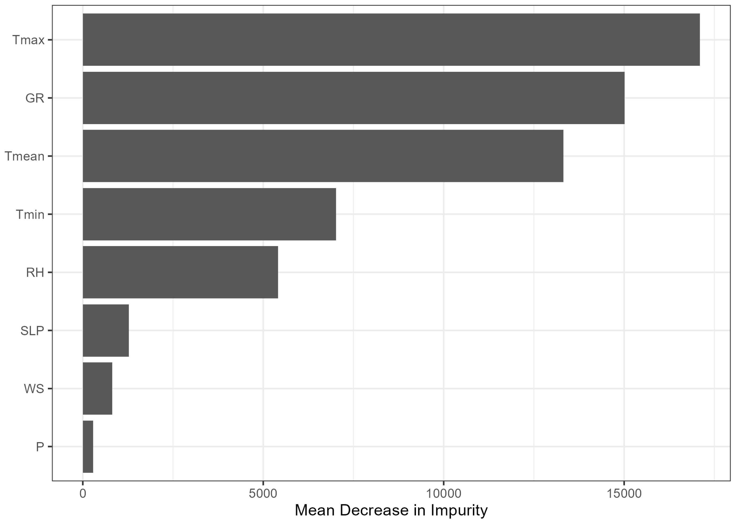
The performance metrics in Table 3 and Supplementary Table S1 (see Supplementary Materials) illustrate a clear decline in model accuracy as the number of input variables decreases, emphasizing the importance of input diversity for machine learning based ET₀ estimation. Accordingly, not all variables have the same importance and information in it regarding the estimation of ET₀. Therefore, we assessed the importance of variables using the Random Forest mean decrease in impurity criterion (Figure 6).

The feature importance analysis showed that maximum temperature (T_max; importance = 17,099) and global radiation (GR; 15,015) were the most influential predictors of ET₀, followed by mean temperature (T_mean; 13,319) and minimum temperature (T_min; 7016). Relative humidity (RH; 5408) also contributed substantially to model performance, whereas sea-level pressure (SLP; 1281), wind speed (WS; 814), and precipitation (P; 284) exhibited comparatively lower importance values.

These findings are physically consistent with the nature of evapotranspiration processes, which are primarily governed by surface energy availability (represented by radiation and temperature-related variables) and atmospheric moisture conditions (partly reflected by RH). The dominance of radiation and temperature variables additionally explains why the machine learning models retained high predictive accuracy even under reduced input scenarios that included only temperature and radiation related predictors (S3–S7). After removing the GR from the feature set, and retaining only T_max (S8), the significant drop in performance off all models is observed. Accordingly, the configuration that included only T_max as the input variable achieved the best performance among single-input models, with R² = 0.85, NSE = 85.01%, RMSE = 0.68 mm/day, and MAE = 0.53 mm/day. Although it outperformed other single-variable configurations, its accuracy remained substantially lower than that of multi input scenarios. This outcome underscores the limitations of using a single meteorological parameter for estimating ET₀, as such models fail to capture the full complexity of ET dynamics. A gradual decline in performance was evident with the reduction in input dimensionality, as indicated by increasing RMSE and decreasing R² values.

The analysis indicates that ANN models are capable of generating highly accurate ET₀ estimates, especially when provided with a diverse set of meteorological inputs. These results are consistent with the findings reported by Makwana et al. [41], who demonstrated that ANN models with five input variables (T_max, T_min, RH, WS, BSS) outperformed simpler configurations and showed strong agreement with FAO-56 PM estimates. Their study also identified T_max as the most influential variable. Also, Dimitriadou and Nikolakopoulos [40] evaluated and compared nineteen Multi-Layer Perceptron (MLP) and Radial Basis Function (RBF) models against ET₀ values estimated using the FAO-56 PM method. The models were developed using different combinations of meteorological input variables, ranging from two to seven parameters. Their results demonstrated high predictive accuracy, with R² values ranging from 0.961 to 0.980, which is comparable to the performance achieved in the present study. Similar, Naresh et al. [42] evaluated the performance of ANN models for estimating ET₀ in the semi-arid region of Haryana State, India. Daily meteorological data collected during the period 2011–2020, including maximum and minimum air temperature, relative humidity, wind speed, and sunshine duration, were used as model inputs. The ANN results were compared with the standard FAO-56 PM method. The authors reported that the best-performing ANN configuration was obtained using the Levenberg–Marquardt (LM) training algorithm with a single hidden layer consisting of 13 neurons, achieving an R² value of 0.986, which is very similar to the accuracy obtained in the present study.

El-Magd et al. [43] demonstrated that ANN models achieved high predictive accuracy when temperature-related variables were included among the input parameters, which is consistent with the findings of the present study. Similarly, Kumar et al. [45] found that ANN models achieved the highest predictive accuracy when all available meteorological input parameters were included, while reduced input combinations resulted in lower model performance. A similar trend was observed in the present study, where the best ANN performance was achieved using a larger number of meteorological variables, whereas model accuracy gradually decreased as the number of input parameters was reduced. Comparable conclusions were presented by Skhiri et al. [46], who showed that ANN models provided accurate ET₀ estimates based on available meteorological data and identified temperature-related variables as highly influential for model performance. These findings are in agreement with the results obtained in the present study, where temperature variables were also among the most important inputs for accurate ET₀ prediction. Shu et al. [20] also emphasized the potential of machine learning approaches for improving ET₀ estimation in data-deficient regions through parameter optimization and regionalization techniques. Their findings further support the applicability of machine learning-based methods for reliable ET₀ estimation under conditions of limited meteorological data availability.

Raimondi et al. [51] evaluated both linear (multiple linear regression, Lasso, Ridge, and Elastic Net) and non-linear machine learning models (regression tree, random forest, XGBoost, support vector regression—SVR, and artificial neural networks—ANNs) for ET₀ estimation across sixteen meteorological stations located in the climatically heterogeneous Veneto region of Italy. The study utilized daily meteorological data for the period 1994–2022, including air temperature, solar radiation, precipitation, and relative humidity. Model performance was benchmarked against the FAO-56 PM equation. Among the tested approaches, SVR, XGBoost, and ANN demonstrated the best predictive capabilities, with R² and NSE values close to 0.96, which was also almost identical to present study.

Although numerous studies have confirmed the high potential of machine learning and ANN approaches for ET₀ estimation, most developed models are region-specific and calibrated under particular climatic conditions. Consequently, their direct application to regions with different climatic and environmental characteristics may be limited, highlighting the importance of developing and validating local or regionally adapted ET₀ prediction models.

For Serbia, Gocić et al. [52] also applied ANN models for the estimation of ET₀. In their study, the FAO-56 PM equation was used as the reference method for ET₀ calculation based on meteorological data collected during the period 1980–2010. However, the ANN models developed in their research achieved lower predictive performance (R² = 0.911) compared to the ANN model obtained in the present study. Similarly, Gocić and Arab Amiri [53] developed ANN models for predicting monthly ET₀ time series using different time lags at six meteorological stations in Serbia for the period 1980–2010. For the Novi Sad meteorological station, three ANN models with different time lags were tested, achieving R² values of 0.81, 0.93, and 0.95, respectively. Although satisfactory results were obtained, the performance of the models remained lower than that achieved in the present study. The improved accuracy obtained in this research may be attributed to the use of a larger and more recent dataset (in our study from 1950 to 2023) and different ANN architectures.

Reference evapotranspiration is an important component of the hydrological cycle and agricultural water management. Accurate estimation of ET₀ plays a crucial role in understanding environmental changes and hydrological processes, particularly in crop irrigation scheduling and water resources management at the river basin scale. As a key variable in agro-hydrological applications, ET₀ estimation is often challenged by the high cost and complexity of direct measurements, as well as by the extensive meteorological data requirements of indirect methods, such as FAO-56 PM. Therefore, the results obtained in this study can be used to manage irrigation scheduling and estimate water balance in more precise and cost efficient way for farmers in Serbia.

4. Conclusions

This study evaluated the effectiveness of ANN models in estimating ET₀ using meteorological data from the Novi Sad station (Vojvodina, Serbia). Various input combinations and ANN architectures were tested and compared with the FAO-56 PM method. The results showed that ANN models can accurately predict ET₀, especially when a larger number of meteorological parameters is included. The highest performance was achieved using all eight input variables (T_max, T_min, T_mean, RH, WS, GR, P, SLP) with a two-hidden-layer structure, resulting in R² = 0.97, NSE = 97.07%, RMSE = 0.23 mm/day, and MAE = 0.21 mm/day. This result suggests that model accuracy improves with greater input diversity and proper network design. Models with reduced input sets also demonstrated satisfactory performance, particularly those including some of the temperature and radiation features (S1–S7). GR prove to be very important variable, which carries a lot of information important for the estimation of the ET₀. After removal of GR the performance of all machine learning model is significantly reduced (S8). The findings confirm the potential of ANN models as reliable tools for ET₀ estimation, indicating their suitability for application in regions with limited meteorological data availability. Future research could explore the application of additional ML models, incorporate data from multiple meteorological stations, and include time series analysis to further improve ET₀ estimation accuracy.

References

1. Thomas, A. Development and Properties of 0.25-Degree Gridded Evapotranspiration Data Fields of China for Hydrological Studies. J. Hydrol. 2008, 358, 145–158. [Google Scholar] [CrossRef]
2. Komatsu, H.; Kume, T.; Otsuki, K. The Effect of Converting a Native Broad-Leaved Forest to a Coniferous Plantation Forest on Annual Water Yield: A Paired-Catchment Study in Northern Japan. For. Ecol. Manag. 2008, 255, 880–886. [Google Scholar] [CrossRef]
3. McVicar, T.R.; Roderick, M.L.; Donohue, R.J.; Li, L.T.; Van Niel, T.G.; Thomas, A.; Grieser, J.; Jhajharia, D.; Himri, Y.; Mahowald, N.M.; et al. Global Review and Synthesis of Trends in Observed Terrestrial Near-Surface Wind Speeds: Implications for Evaporation. J. Hydrol. 2012, 416–417, 182–205. [Google Scholar] [CrossRef]
4. Lin, P.; He, Z.; Du, J.; Chen, L.; Zhu, X.; Li, J. Impacts of Climate Change on Reference Evapotranspiration in the Qilian Mountains of China: Historical Trends and Projected Changes. Int. J. Climatol. 2018, 38, 2980–2993. [Google Scholar] [CrossRef]
5. Saggi, M.K.; Jain, S. Reference Evapotranspiration Estimation and Modeling of the Punjab Northern India Using Deep Learning. Comput. Electron. Agric. 2019, 156, 387–398. [Google Scholar] [CrossRef]
6. Patil, A.P.; Deka, P.C. An Extreme Learning Machine Approach for Modeling Evapotranspiration Using Extrinsic Inputs. Comput. Electron. Agric. 2016, 121, 385–392. [Google Scholar] [CrossRef]
7. Kumar, M.; Raghuwanshi, N.S.; Singh, R.; Wallender, W.W.; Pruitt, W.O. Estimating Evapotranspiration Using Artificial Neural Network. J. Irrig. Drain. Eng. 2002, 128, 224–233. [Google Scholar] [CrossRef]
8. Jahanbani, H.; El-Shafie, A.H. Application of Artificial Neural Network in Estimating Monthly Time Series Reference Evapotranspiration with Minimum and Maximum Temperatures. Paddy Water Environ. 2011, 9, 207–220. [Google Scholar] [CrossRef]
9. Abdullahi, J.; Elkiran, G. Prediction of the Future Impact of Climate Change on Reference Evapotranspiration in Cyprus Using Artificial Neural Network. Procedia Comput. Sci. 2017, 120, 276–283. [Google Scholar] [CrossRef]
10. Trajkovic, S.; Kolakovic, S. Evaluation of Reference Evapotranspiration Equations under Humid Conditions. Water Resour. Manag. 2009, 23, 3057–3067. [Google Scholar] [CrossRef]
11. Allen, R.G.; Pereira, L.S.; Raes, D.; Smith, M. Crop Evapotranspiration: Guidelines for Computing Crop Water Requirements; FAO Irrigation and Drainage Paper No. 56; Food and Agriculture Organization (FAO): Rome, Italy, 1998. [Google Scholar]
12. Fisher, D.K.; Pringle, H.C., III. Evaluation of Alternative Methods for Estimating Reference Evapotranspiration. Agric. Sci. 2013, 4, 51–60. [Google Scholar] [CrossRef]
13. Milly, P.C.D.; Dunne, K.A. Potential Evapotranspiration and Continental Drying. Nat. Clim. Change 2016, 6, 946–949. [Google Scholar] [CrossRef]
14. Zhu, B.; Feng, Y.; Gong, D.; Jiang, S.; Zhao, L.; Cui, N. Hybrid Particle Swarm Optimization with Extreme Learning Machine for Daily Reference Evapotranspiration Prediction from Limited Climatic Data. Comput. Electron. Agric. 2020, 173, 105430. [Google Scholar] [CrossRef]
15. Chia, M.Y.; Huang, Y.F.; Koo, C.H. Support Vector Machine Enhanced Empirical Reference Evapotranspiration Estimation with Limited Meteorological Parameters. Comput. Electron. Agric. 2020, 175, 105577. [Google Scholar] [CrossRef]
16. Basso, B.; Martinez-Feria, R.A.; Rill, L.; Ritchie, J.T. Contrasting Long-Term Temperature Trends Reveal Minor Changes in Projected Potential Evapotranspiration in the US Midwest. Nat. Commun. 2021, 12, 1476. [Google Scholar] [CrossRef]
17. Tabari, H.; Grismer, M.E.; Trajkovic, S. Comparative Analysis of 31 Reference Evapotranspiration Methods under Humid Conditions. Irrig. Sci. 2013, 31, 107–117. [Google Scholar] [CrossRef]
18. Kisi, O.; Sanikhani, H.; Zounemat-Kermani, M.; Niazi, F. Long-Term Monthly Evapotranspiration Modeling by Several Data-Driven Methods without Climatic Data. Comput. Electron. Agric. 2015, 115, 66–77. [Google Scholar] [CrossRef]
19. Zhang, D.; Lin, J.; Peng, Q.; Wang, D.; Yang, T.; Sorooshian, S.; Liu, X.; Zhuang, J. Modeling and Simulating of Reservoir Operation Using the Artificial Neural Network, Support Vector Regression, Deep Learning Algorithm. J. Hydrol. 2018, 565, 720–736. [Google Scholar] [CrossRef]
20. Shu, Z.; Zhou, Y.; Zhang, J.; Jin, J.; Wang, L.; Cui, N.; Wang, G.; Zhang, J.; Wu, H.; Wu, Z.; et al. Parameter Regionalization Based on Machine Learning Optimizes the Estimation of Reference Evapotranspiration in Data Deficient Area. Sci. Total Environ. 2022, 844, 157034. [Google Scholar] [CrossRef]
21. Monteith, J.L. Evaporation and environment. In The State and Movement of Water in Living Organisms; Proceedings of the 19th Symposium of the Society for Experimental Biology; Cambridge University Press: Cambridge, UK, 1965; pp. 205–234. [Google Scholar]
22. Droogers, P.; Allen, R.G. Estimating Reference Evapotranspiration under Inaccurate Data Conditions. Irrig. Drain. Syst. 2002, 16, 33–45. [Google Scholar] [CrossRef]
23. Trajkovic, S. Hargreaves versus Penman-Monteith under Humid Conditions. J. Irrig. Drain. Eng. 2007, 133, 38–42. [Google Scholar] [CrossRef]
24. Traore, S.; Wang, Y.-M.; Kerh, T. Artificial Neural Network for Modeling Reference Evapotranspiration Complex Process in Sudano-Sahelian Zone. Agric. Water Manag. 2010, 97, 707–714. [Google Scholar] [CrossRef]
25. Almorox, J.; Quej, V.H.; Martí, P. Global Performance Ranking of Temperature-Based Approaches for Evapotranspiration Estimation Considering Köppen Climate Classes. J. Hydrol. 2015, 528, 514–522. [Google Scholar] [CrossRef]
26. Feng, Y.; Cui, N.; Zhao, L.; Hu, X.; Gong, D. Comparison of ELM, GANN, WNN and Empirical Models for Estimating Reference Evapotranspiration in Humid Region of Southwest China. J. Hydrol. 2016, 536, 376–383. [Google Scholar] [CrossRef]
27. Jayashree, T.R.; Reddy, N.V.S.; Acharya, U.D.; Eslamian, S. Prediction of Reference Crop Evapotranspiration: Empirical and Machine Learning Approaches. In Handbook of Hydroinformatics; Elsevier: Amsterdam, The Netherlands, 2023; pp. 253–268. ISBN 9780128219614. [Google Scholar]
28. Rahimi Khoob, A. Comparative Study of Hargreaves’s and Artificial Neural Network’s Methodologies in Estimating Reference Evapotranspiration in a Semiarid Environment. Irrig. Sci. 2008, 26, 253–259. [Google Scholar] [CrossRef]
29. Dai, X.; Shi, H.; Li, Y.; Ouyang, Z.; Huo, Z. Artificial Neural Network Models for Estimating Regional Reference Evapotranspiration Based on Climate Factors. Hydrol. Process. 2009, 23, 442–450. [Google Scholar] [CrossRef]
30. Kumar, M.; Raghuwanshi, N.S.; Singh, R. Artificial Neural Networks Approach in Evapotranspiration Modeling: A Review. Irrig. Sci. 2011, 29, 11–25. [Google Scholar] [CrossRef]
31. Martí, P.; Royuela, A.; Manzano, J.; Palau-Salvador, G. Generalization of Eto Ann Models through Data Supplanting. J. Irrig. Drain. Eng. 2010, 136, 161–174. [Google Scholar] [CrossRef]
32. Pour-Ali Baba, A.; Shiri, J.; Kisi, O.; Fard, A.F.; Kim, S.; Amini, R. Estimating Daily Reference Evapotranspiration Using Available and Estimated Climatic Data by Adaptive Neuro-Fuzzy Inference System (Anfis) and Artificial Neural Network (Ann). Hydrol. Res. 2013, 44, 131–146. [Google Scholar] [CrossRef]
33. Antonopoulos, V.Z.; Antonopoulos, A.V. Daily Reference Evapotranspiration Estimates by Artificial Neural Networks Technique and Empirical Equations Using Limited Input Climate Variables. Comput. Electron. Agric. 2017, 132, 86–96. [Google Scholar] [CrossRef]
34. Ferreira, L.B.; Da Cunha, F.F.; De Oliveira, R.A.; Fernandes Filho, E.I. Estimation of Reference Evapotranspiration in Brazil with Limited Meteorological Data Using ANN and SVM—A New Approach. J. Hydrol. 2019, 572, 556–570. [Google Scholar] [CrossRef]
35. Jyothi; Reddy, G.V.S.; Babu, B.M.; Kulkarni, P.S.; Ananda, N. Artificial Neural Network Models for Estimation of Potential Evapotranspiration in a Semi-Arid Region of Raichur, Karnataka. J. Agric. Eng. 2020, 57, 172–181. [Google Scholar] [CrossRef]
36. Kisi, O. Generalized Regression Neural Networks for Evapotranspiration Modelling. Hydrol. Sci. J. 2006, 51, 1092–1105. [Google Scholar] [CrossRef]
37. Landeras, G.; Ortiz-Barredo, A.; López, J.J. Comparison of Artificial Neural Network Models and Empirical and Semi-Empirical Equations for Daily Reference Evapotranspiration Estimation in the Basque Country (Northern Spain). Agric. Water Manag. 2008, 95, 553–565. [Google Scholar] [CrossRef]
38. Walczak, S.; Cerpa, N. Artificial Neural Networks. In Encyclopedia of Physical Science and Technology; Elsevier: Amsterdam, The Netherlands, 2003; pp. 631–645. ISBN 9780122274107. [Google Scholar]
39. Mallikarjuna, P.; Jyothy, S.A.; Sekhar Reddy, K.C. Daily Reference Evapotranspiration Estimation Using Linear Regression and Ann Models. J. Inst. Eng. India Ser. A 2012, 93, 215–221. [Google Scholar] [CrossRef]
40. Dimitriadou, S.; Nikolakopoulos, K.G. Artificial Neural Networks for the Prediction of the Reference Evapotranspiration of the Peloponnese Peninsula, Greece. Water 2022, 14, 2027. [Google Scholar] [CrossRef]
41. Makwana, J.J.; Deora, B.S.; Parmar, B.S.; Patel, C.K.; Saini, A.K. Modelling of Reference Evapotranspiration Using Artificial Neural Network in Semi-Arid Region of North Gujarat. J. Agric. Eng. 2022, 59, 193–200. [Google Scholar] [CrossRef]
42. Naresh, R.; Kumar, M.; Kumar, S.; Singh, K.; Sharma, P. Estimation of Reference Evapotranspiration Using Artificial Neural Network Models for Semi-Arid Region of Haryana. J. Agrometeorol. 2023, 25, 145–150. [Google Scholar] [CrossRef]
43. El-Magd, A.A.; Baraka, S.M.; Eid, S.F.M. Using artificial neural networks to predict the reference evapotranspiration. J. Water Land Dev. 2023, 57, 1–8. [Google Scholar] [CrossRef]
44. Makwana, J.J.; Tiwari, M.K.; Deora, B.S. Development and Comparison of Artificial Intelligence Models for Estimating Daily Reference Evapotranspiration from Limited Input Variables. Smart Agric. Technol. 2023, 3, 100115. [Google Scholar] [CrossRef]
45. Kumar, S.; Sharda, R.; Goyal, P.; Siag, M.; Kaur, P. Reference Evapotranspiration Modelling Using Artificial Neural Networks under Scenarios of Limited Weather Data: A Case Study in the Malwa Region of Punjab. Environ. Model. Assess. 2024, 29, 589–620. [Google Scholar] [CrossRef]
46. Skhiri, A.; Ferhi, A.; Bousselmi, A.; Khlifi, S.; Mattar, M.A. Artificial Neural Network for Forecasting Reference Evapotranspiration in Semi-Arid Bioclimatic Regions. Water 2024, 16, 602. [Google Scholar] [CrossRef]
47. Copernicus Climate Change Service (C3S). Climate Data and Services. Implemented by ECMWF as Part of the Copernicus Programme. Available online: https://climate.copernicus.eu (accessed on 6 February 2024).
48. Jensen, M.E.; Burman, R.D.; Allen, R.G. (Eds.) Evapotranspiration and Irrigation Water Requirements; American Society of Civil Engineers (ASCE): New York, NY, USA, 1990. [Google Scholar]
49. Maier, H.R.; Dandy, G.C. Neural Networks for the Prediction and Forecasting of Water Resources Variables: A Review of Modelling Issues and Applications. Environ. Model. Softw. 2000, 15, 101–124. [Google Scholar] [CrossRef]
50. Liakos, K.; Busato, P.; Moshou, D.; Pearson, S.; Bochtis, D. Machine Learning in Agriculture: A Review. Sensors 2018, 18, 2674. [Google Scholar] [CrossRef] [PubMed]
51. Raimondi, G.; Bonato, J.; Maucieri, C. Machine Learning Models for Reference Evapotranspiration Estimation in New Locations under Data-Limited Conditions in Northeastern Italy. Eur. J. Agron. 2026, 178, 128132. [Google Scholar] [CrossRef]
52. Gocić, M.; Motamedi, S.; Shamshirband, S.; Petković, D.; Ch, S.; Hashim, R.; Arif, M. Soft Computing Approaches for Forecasting Reference Evapotranspiration. Comput. Electron. Agric. 2015, 113, 164–173. [Google Scholar] [CrossRef]
53. Gocić, M.; Arab Amiri, M. Reference Evapotranspiration Prediction Using Neural Networks and Optimum Time Lags. Water Resour. Manag. 2021, 35, 1913–1926. [Google Scholar] [CrossRef]
Figure 1. Location of the meteorological station used in the study.
Earth 07 00088 g001
Figure 2. Mean values of the meteorological variables at the Novi Sad station for the period from 1950 to June 2023.
Earth 07 00088 g002
Figure 3. Architecture of the ANN model.
Earth 07 00088 g003
Figure 4. Multi-year average daily ET0 at the Novi Sad station for the period 1950–2023.
Earth 07 00088 g004
Figure 5. Pairplot of meteorological variables used as inputs for ET0 modeling, showing scatter plots below the diagonal and variable distributions along the diagonal.
Earth 07 00088 g005
Figure 6. Variable importance (mean decrease in impurity).
Earth 07 00088 g006