SAR-Based Flood Extent Mapping with a Lightweight Siamese U-Net and Differential Attention Mechanism

Abstract

Floods are among the most catastrophic natural disasters globally, causing significant damage to both life and infrastructure. Consequently, immediate and accurate assessment of inundated areas is critical for effective emergency response. While optical remote sensing is typically used for flood assessment, it is often ineffective during active flood events due to persistent cloud cover and precipitation. To address this, this research develops a deep learning method utilizing Synthetic Aperture Radar (SAR), which offers all-weather, 24 h imaging capabilities. Specifically, an attention-based differential Siamese U-Net was developed to detect temporal changes in bi-temporal SAR imagery (e.g., Sentinel-1) acquired before and after flood events. The method was evaluated on the S1GFloods dataset, comprising 5360 bi-temporal Sentinel-1 SAR image pairs across 46 flood incidents on six continents. Experimental results demonstrate a flood Intersection over Union (IoU) of 92.43%, an F1 score of 96.07%, and a recall of 97.64%. These metrics rank the proposed approach third overall among top-performing methods on this dataset. Notably, the high recall rate indicates the model is particularly beneficial for emergency response, as it minimizes the number of undetected flooded areas. Despite utilizing a CNN-based architecture that is less complex than Vision Transformer models, this method achieves results comparable to the state-of-the-art DAM-Net, with a performance difference of only 0.77%.

1. Introduction

Floods are known as one of the most destructive natural events worldwide, resulting in significant casualties, widespread infrastructure collapse, and substantial economic deficits [1,2]. According to recent estimates, flood disasters affect millions of people annually and account for a significant proportion of natural disaster-related casualties. The ability to rapidly and accurately delineate flood extents is essential for emergency response coordination, evacuation planning, damage assessment, and post-disaster recovery efforts.

Past methods of monitoring floods, such as conducting site visits, rely on in-field data collection and are therefore plagued by serious obstacles to their implementation during actual flood events: field staff are frequently denied access to flooded areas; the risk to field personnel is extremely high; and ground surveys can only cover a small portion of the area. Further, since the flood evolves rapidly, there is a need to collect new data at relatively short time intervals, which cannot be accomplished using traditional ground-based methods.

Satellite remote sensing offers an indispensable tool for the monitoring of flood events, capable of providing large-scale and frequent synoptic coverage of affected areas. Optical satellites like Sentinel-2 and Landsat produce high-resolution, multispectral images that are well-suited for defining boundaries of bodies of water (in the absence of cloud cover) [3]. The principal drawback limiting the usefulness of optical sensors for flood mapping is that the type of weather that causes the majority of flooding (heavy rainfall) typically results in thick cloud cover that blocks line-of-sight between the satellite and the Earth’s surface. Past studies indicate that up to 80 percent of optical imagery collected during floods is contaminated by clouds—at a time when it is most critical to collect flood-related information.

Because SAR is an active microwave sensing system, it can capture data and images without being affected by atmospheric conditions that typically limit optical imagery. As such, SAR sensors use microwaves (in the electromagnetic spectrum; wavelengths of 1 cm to 1 m) to transmit energy and receive the backscattered signals as they reflect off the Earth’s surface [4]. The active nature of SAR enables it to collect imagery regardless of solar illumination, thus enabling daytime and nighttime observation capabilities. Additionally, microwave energy used in SAR systems (such as C-, L-, and X-bands) can penetrate clouds, rain, and aerosols, enabling reliable “all-weather” data collection for many disaster-response applications [5].

The physical basis for detecting water bodies in SAR imagery lies in the way smooth surfaces reflect incident microwave signals. Water with no ripples will create specular reflections from the sensor, which will result in all the incoming energy being scattered away from the sensor in a mirrored way because of the surface’s smoothness compared to the radar frequency wavelength; thus, there is very little backscattered energy returned to the sensor, so water bodies will be identified by their characteristic “dark” appearance in the SAR imagery [4]. In the SAR image, the contrast between the relatively low-backscattered water surfaces and the relatively high-backscattered terrain surrounding the water surfaces is the basic signature used to develop SAR-based algorithms to detect flooding [6].

Under the Copernicus Programme, the ESA has significantly improved the operational use of SAR for flood monitoring through the Sentinel-1 mission [7]. Two satellite systems, namely, Sentinel-1A and Sentinel-1B, provide high-quality C-band SAR imagery with a revisit cycle of less than six days (and shorter where higher latitude exists), 10 m spatial resolution, and dual polarization capability (VV/VH). The Sentinel-1 mission is also characterized by its free and openly available data—thus, it can be used globally—and by its systematic image acquisition pattern that guarantees availability of baseline images to support all change-detection methods [8]. Due to these characteristics, Sentinel-1 has become the widely utilized source of data for flood monitoring services in operation worldwide, and specifically for The Global Flood Monitoring (GFM) product provided by the Copernicus Emergency Management Service [9].

SAR is inherently advantageous for flood mapping; however, the ability to accurately delineate flood extent using SAR data is limited by several technical challenges. The first challenge is speckle noise, which is an inherent part of the data obtained when using coherent imaging systems. Speckle causes a “grainy” effect in the image data that creates difficulties with identifying boundaries and can make it difficult to use a threshold as a basis for detecting flooding [4]. A second challenge arises from land cover types that produce radar backscatter similar to water bodies, such as smooth asphalt, airport runways, mountain shadows, and certain moist bare soils, which can lead to false flood detections [1].

Detecting floods in urban areas is particularly challenging due to the dihedral scattering mechanism that occurs when floodwaters are on the street in between two or more buildings. The radar signal will be reflected off the top of the flood waters (specular) and then off an adjacent building wall, which returns with much greater strength to the sensor [10,11]. This phenomenon makes it difficult to detect flooding in urban environments as these areas typically appear brighter than they were before the flood, contrary to what is generally anticipated—complicating development of detection algorithms based upon the dark water signature.

Deep learning techniques have provided significant improvements in this area by providing a method to learn and represent features of flood signals in an approach that is able to differentiate between true flood signals and noise/confounding factors [12]. Deep Learning Techniques (such as CNNs) have seen wide use in SAR Flood Detection where many are using U-Net architectures to perform well in tasks such as semantic segmentation [13]. More recent developments with the use of Vision Transformers (ViTs) have achieved high levels of performance on benchmarking SAR flood detection [14], as they are able to capture relationships between spatial features over larger distances.

This work proposes a Siamese U-Net architecture together with a Differential Attention mechanism for bi-temporal SAR flood detection. The approach is designed to exploit the change-detection paradigm, comparing post-flood and pre-flood image pairs to determine newly inundated regions while suppressing permanent water bodies and false alarm sources. Our contributions are summarized below:

(1) Siamese decoder and encoder architecture with weight-shared branches is proposed, employing a simplified Differential Attention module that explicitly models temporal change features through learned attention weights.

(2) Comprehensive experimental evaluation is conducted on the S1GFloods dataset, demonstrating competitive performance with state-of-the-art methods while maintaining architectural simplicity.

(3) Offering a high-recall flood-detection framework to advance SAR-based flood mapping with a model specifically suited for emergency response contexts that prioritize minimizing missed inundation regions.

2. Study Area and Dataset

2.1. S1GFloods Dataset Overview

The research was conducted using the S1GFloods dataset (Saleh et al., 2024) [14,15], which represents a major improvement to SAR-based flood detection benchmarks. The S1GFloods dataset provides greater geographical coverage and a greater variety of flood events than previous datasets, making it ideal for developing new deep learning models. Data used to create the S1GFloods dataset were obtained using Sentinel-1 GRD IW-mode acquisitions.

The S1GFloods dataset includes 5360 bi-temporal image pairs (i.e., 10,720 individual SAR images organized into pre-flood and post-flood pairs) produced from the satellite Sentinel-1. Each pair of images was taken at two different times (pre and post) of an event involving flooding and has been annotated using ground-truth maps of the flooded areas created by experts. The S1GFloods dataset captures 46 flood events distributed among six continents over a time span of 7 years (from 2015 to 2022). Because of its global scope, this dataset ensures that all training models will be able to generalize to different geographical contexts as well as flood types and land cover classifications. It is important to clarify that S1GFloods is distinct from the earlier Sen1Floods11 dataset of Bonafilia et al. [3]: while Sen1Floods11 provides 4831 single-temporal Sentinel-1 chips for one-time flood segmentation, S1GFloods provides 5360 bi-temporal pre-flood/post-flood pairs specifically constructed for change-detection learning. The present study uses only the S1GFloods dataset.

The S1GFloods dataset includes six flood-type categories: heavy rainfall (HR), overflowing rivers (ORs), broken dams (BDs), cyclones (e.g., Cyclone Shaheen CS), tropical storms (TSs), and inundation caused by hurricanes (Hs). These different flood categories ensure that the trained model will experience a variety of flooding patterns, progressions and associated land cover characteristics. Examples of affected landscapes include: urban/rural settlements; wetlands and riverine corridors; mountainous landscapes; agricultural/land vegetation; and coastal zones. Representative sample image pairs from the S1GFloods dataset are illustrated in Figure 1.

2.2. Data Preprocessing Pipeline

The creators of the S1GFloods dataset used the ESA’s Python version of the snappy toolkit [14], the Python API for the Sentinel Application Platform (SNAP), to preprocess the dataset. A description of the processing workflow executed on the Sentinel-1 GRD data can be found in

Table 1. Preprocessing chain applied to S1GFloods.

Step	Process	Purpose
1	Orbital Correction	Precise satellite positioning using POD files
2	Thermal Noise Correction	Subtraction of sensor-generated thermal noise
3	Border Noise Correction	Elimination of artifacts along image edges
4	Radiometric Calibration	Conversion to σ0 backscatter coefficient
5	Terrain Correction	Geometric correction using Range Doppler with DEM
6	Decibel Conversion	Logarithmic scaling: σdB0 = 10 × log10(σ0)
7	Normalization	Scaling from dB range to 8-bit PNG (0–255)

.

Radiometric calibration is necessary for all forms of quantitative analysis, as it transforms the sensor-dependent digital numbers (DNs) into a physical radiometric quantity of measure of surface reflectivity (normalized by the illuminated area). Calibration is accomplished through conversion to the sigma nought (σ⁰) backscattering coefficient. Topographic correction or terrain correction is needed to correct for distortion resulting from topography, which would result in inaccurate positioning on a map of any feature that is detected.

One of the most important decisions made during the preprocessing of the S1GFloods dataset was to intentionally avoid filtering out speckle. Traditional SAR processing workflows apply spatial filters (Lee, Frost, Gamma-MAP) to reduce speckle noise at the cost of spatial resolution loss. The dataset creators elected to preserve the original speckle characteristics, allowing deep learning models to learn speckle-robust feature representations directly from the data rather than relying on potentially information-destructive filtering operations [14].

Ground-truth labels were generated through a semiautomated process. Initial water masks were produced using an established backscatter threshold of σ⁰ = −18 dB, a value commonly employed for water body detection in C-band SAR imagery. These initial masks were subsequently refined by skilled remote sensing interpreters using contemporaneous high-resolution optical imagery as reference, ensuring label accuracy for model training.

2.3. Dataset Partition

The dataset was split into training, validation, and test subsets as specified in

Table 2. Dataset partition.

Subset	Samples	Percentage
Training	3751	70%
Validation	804	15%
Test	805	15%

. It is important to emphasize that this partition differs from the original 80/10/10 split employed by Saleh et al. [14]. The larger validation and test sets in the present study were selected to provide more robust performance estimation. Random sampling was used for partitioning, consistent with the proportional split strategy used in the original S1GFloods study, which distributes samples from each flood event across all subsets to ensure representation of all flood types while maintaining temporal pairing constraints [14]. As noted by recent benchmark analyses [16], this approach, common among SAR flood detection datasets, poses a risk of spatial autocorrelation between training and test samples, though it ensures fair comparison with prior work on this benchmark.

2.4. Comparison with Existing Flood Detection Datasets

The S1GFloods dataset offers the greatest diversity in terms of flood event coverage and geographic distribution among existing benchmarks [15], making it particularly suitable for developing models with strong generalization capabilities.

Table 3. Flood detection datasets.

Dataset	Pairs	Size	Events	Period
MM-Flood	1748	2000 × 2000	42	2014–2021
SEN12-FLOOD	336	512 × 512	–	2018–2019
Sen1Floods11	4831	512 × 512	11	2016–2019
ETCI-2021	33405	256 × 256	5	2017–2019
S1GFloods	5360	256 × 256	46	2015–2022

presents a comparison of S1GFloods dataset with other publicly available SAR flood detection datasets [17,18].

3. Methodology

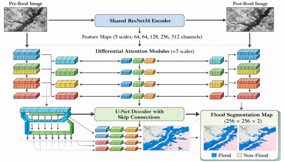
The proposed method employs a Siamese encoder–decoder architecture for bi-temporal SAR image analysis. The network architecture, illustrated in Figure 2, comprises three principal components: (1) shared encoder that extracts multi scale features from both pre-flood and post-flood images; (2) Differential Attention modules that compute change features at multiple spatial scales; and (3) U-Net decoder generates the final flood segmentation map.

The bi-temporal approach utilizes a change-detection strategy to compare pre-flood and post-flood event images; by doing so, it allows for an identification of permanent water bodies corresponding to those that are present in both the pre-event and post-event images and the flood-affected areas as those that appear only in the post-event images. Using this temporal differencing method significantly reduces the amount of false positive identifications resulting from permanent water bodies.

3.1. Siamese Encoder

ResNet34, which is a representation learning model [19,20], is used as an encoder initialized with pre-trained weights on the ImageNet dataset. This architecture was selected because it offers a good trade-off between representational capability and computational cost and has been demonstrated to be successful for numerous remote sensing applications. Using pre-trained weights on ImageNet data, although there are domain differences between ImageNet data and SAR data, the prior work [12] demonstrated that this approach accelerates convergence and improves generalization in the task of remote sensing semantic segmentation.

The Siamese architecture shares weights between two separate but parallel encoding paths which process pre-flood and post-flood imagery to enable a similar transformation on each path resulting in a consistent representation of features for meaningful time-based comparison to be performed. Weight sharing also reduces the total parameter count compared to independent encoders while providing implicit regularization against overfitting to acquisition-specific artifacts [21].

The encoder produces feature maps at five scales with channel dimensions of [64, 64, 128, 256, 512], corresponding to progressively increasing receptive fields and semantic abstraction levels. Siamese architecture allows for a hierarchical representation of features at multiple scales to allow for capturing detail within boundaries as well as larger contextual elements.

The Sentinel-1 mission acquires data in dual co-/cross-polarization (VV and VH). For this study, the VV (vertical-transmit, vertical-receive) polarization channel was used as the SAR input. This choice is consistent with established practice for SAR-based water body and flood detection, where the VV channel is preferred because smooth water surfaces produce strong specular reflection and consequently very low VV backscatter, yielding the characteristic dark-water signature [5,6]. The S1GFloods dataset [14] further reinforces this choice: ground-truth water masks were generated using a backscatter threshold of σ⁰ = −18 dB, a well-established VV threshold for C-band SAR water detection. To meet the three-channel input requirement of the ImageNet-pre-trained ResNet34 encoder, the single-channel VV intensity image (delivered by the S1GFloods preprocessing pipeline as an 8-bit grayscale PNG) was replicated across the three input channels. The cross-polarized VH channel was not used in the present implementation; explicit dual-polarization processing through a modified two-channel input architecture is identified as a direction for future work (Section 5.2).

3.2. Differential Attention Module

The key differentiator of the proposed system’s architecture is the Differential Attention module. This module represents how two time-based representations are related in order to improve a change-detection performance model. It uses a temporal difference at each encoder level as follows:

$${\mathrm{D}}^{\left(\mathrm{l}\right)}=\left|{\mathrm{F}}_{\mathrm{p}\mathrm{o}\mathrm{s}\mathrm{t}}^{\left(\mathrm{l}\right)}-{\mathrm{F}}_{\mathrm{p}\mathrm{r}\mathrm{e}}^{\left(\mathrm{l}\right)}\right|$$

(1)

Here, F_pre and F_post represent the feature map generated from the pre-flood image and the post-flood image, at scale l. The absolute difference function allows the module to capture the degree of change (i.e., magnitude) without being sensitive to the sign of the intensity difference.

An attention map is subsequently computed to weight the importance of different spatial locations based on both the post-flood features and the detected changes:

$${\mathrm{A}}^{\left(\mathrm{l}\right)}=\mathrm{\sigma }\left(\mathrm{C}\mathrm{o}\mathrm{n}\mathrm{v}\left(\left[{\mathrm{F}}_{\mathrm{p}\mathrm{o}\mathrm{s}\mathrm{t}}^{\left(\mathrm{l}\right)},{\mathrm{D}}^{\left(\mathrm{l}\right)}\right]\right)\right)$$

(2)

where [·,·] denotes channel-wise concatenation, Conv represents a sequence of convolutional layers with batch normalization and ReLU activation, and σ denotes the sigmoid function constraining attention weights to the range [0, 1].

The final change feature map is derived through elementwise multiplication:

$${\mathrm{C}}^{\left(\mathrm{l}\right)}={\mathrm{D}}^{\left(\mathrm{l}\right)}\odot {\mathrm{A}}^{\left(\mathrm{l}\right)}$$

(3)

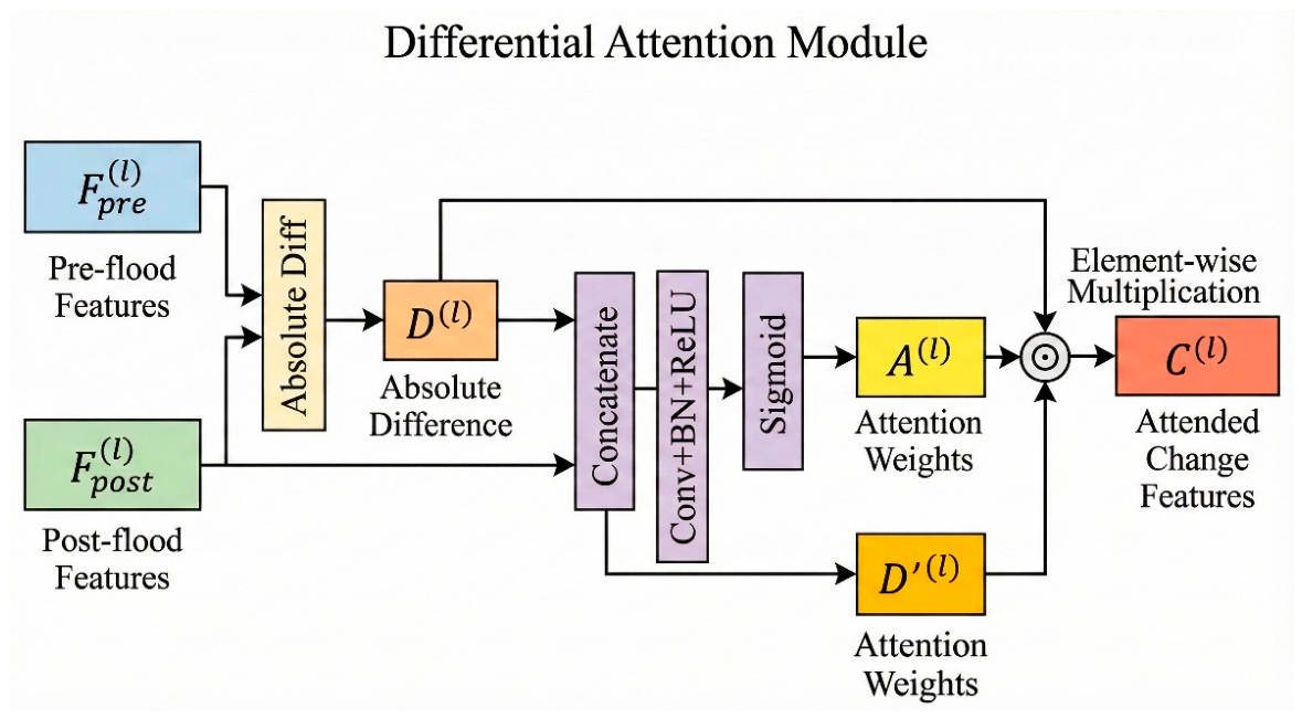
This multiplicative gating mechanism enables the network to emphasize genuine flood-induced changes while suppressing noise and pseudo-changes arising from factors such as varying imaging conditions, seasonal vegetation changes, or speckle variation. The learned attention weights provide an interpretable mechanism for understanding which spatial regions contribute most strongly to the final prediction. The complete design of the Differential Attention module is provided in Figure 3. The module computes absolute difference between bi-temporal features, concatenates with post-flood features, applies convolutional layers with sigmoid activation to generate attention weights, and produces attended change features through element-wise multiplication.

3.3. U-Net Decoder

The decoder follows the established U-Net architecture [13], employing transposed convolutions for spatial up-sampling and skip connections from encoder stages. Skip connections enable fusing low-level spatial information with higher level semantic features, facilitating precise boundary delineation that is critical for accurate flood extent mapping. The decoder configuration is specified in

Table 4. Decoder configuration.

Block	Input Ch.	Output Ch.	Skip
Dec5	512	256	Stage 4
Dec4	256 + 256	128	Stage 3
Dec3	128 + 128	64	Stage 2
Dec2	64 + 64	32	Stage 1
Dec1	32 + 64	16	Stage 0
Head	16	2	–

.

The final segmentation head produces a two-channel output representing background and flood-class probabilities, from which the flood mask is derived through argmax selection.

3.4. Loss Function

The network is trained using a combined loss function that incorporates both region-based and distribution-based objectives:

L_total = λ_dice L_dice + λ_focal L_focal

(4)

where λ_dice = λ_focal = 0.5.

The Dice loss [22] directly optimizes the overlap between segmentation mask predictions and ground-truth segmentation masks:

L_dice = 1 − (2 ∑p_i g_i + ε)/(∑p_i + ∑g_i + ε)

(5)

where p_i and g_i denote the predicted probability and ground-truth label for pixel i, respectively, and ϵ is a smoothing constant to prevent division by zero.

Focal loss [23] was developed to handle class imbalances by reducing the value of correctly classified samples, therefore allowing training to focus on difficult boundary pixel regions and rare classes:

L_focal = −α_t(1 − p_t)^γ log(p_t)

(6)

where γ = 2.0 controls the focusing parameter and α_t provides class weighting.

This loss combination differs from the original DAMNet formulation, which employs Dice loss with a contrastive loss for metric learning. The substitution of Focal loss for contrastive loss changes the training objective from metric learning to hard example mining, which may account for some of the precision–recall trade-off differences observed in experimental results.

3.5. Training Configuration

The AdamW optimizer was selected because its decoupled weight-decay regularization has been shown to improve generalization compared to the original Adam optimizer [24]. The cosine annealing schedule with warm restarts provides periodic increases in learning rate, facilitating escape from suboptimal local minima during training.

Data Augmentation of the training set was only performed with the Albumentations Library [25] as follows: horizontal/vertical flip with a probability of 0.5, random 90-degree rotation with a probability of 0.5, Gaussian blur with a probability of 0.3, Gaussian noise injection with a probability of 0.3.

These data augmentation methods were used in conjunction with all other image types and their respective masks for consistency of spatial correspondence.

The training was completed utilizing a single NVIDIA A100-SXM4-40GB GPU and utilized Mixed Precision Arithmetic (FP16) to minimize memory requirements and maximize computational performance in Google Colab. The training hyperparameters are summarized in

Table 5. Training hyperparameters.

Hyperparameter	Value
Optimizer	AdamW
Initial Learning Rate	1 × 10−4
Weight Decay	1 × 10−4
Batch Size	16
Maximum Epochs	100
Early Stopping Patience	20 epochs
Gradient Clipping	Max norm 1.0
Learning Rate Schedule	Cosine Annealing with Warm Restarts

.

3.6. Evaluation Metrics

These four metrics were used to assess segmentation results:

• Intersection over Union (IoU): IoU measures the amount of intersection in predicted versus ground-truth bounding boxes, defined by the formula IoU = TP/(TP+ FP + FN); TP, FP, and FN represent true positives, false positives and false negatives.
• F1-Score: F1 Score is the average of Precision and Recall to provide a good balance for assessing detection quality; F1 = 2 × (Precision × Recall)/(Precision + Recall).
• Precision: Precision is the ratio of true positive predictions over total number of predicted pixels; Precision = TP/(TP + FP).
• Recall: Recall is the ratio of true positive predictions over total number of actual pixels; Recall = TP/(TP + FN).

4. Results

4.1. Quantitative Results

The segmentation results indicate a high level of accuracy in delineating flooded areas from satellite imagery (

Table 6. Performance on S1GFloods Test Set.

Metric	Value (%)
Flood IoU	92.43
Background IoU	96.13
Mean IoU	94.28
F1-Score (Flood)	96.07
Precision (Flood)	94.55
Recall (Flood)	97.64

). The model achieves a flood IoU of 92.43% and a background IoU of 96.13%, yielding a robust mean IoU of 94.28%. These values suggest that the model is capable of learning well-defined class boundaries and maintaining strong consistency across both foreground (flood) and background classes. The slightly higher IoU for the background class is common in flood-mapping tasks, where background regions tend to be more spatially extensive and less heterogeneous compared to flood-affected areas. The precision of 94.55% indicates that most predicted flooded pixels are correct, while the recall of 97.64% demonstrates that the model is highly sensitive and capable of detecting the majority of true flooded areas. This high recall is particularly important in disaster response, where missed detections can lead to underestimation of affected regions. The slight gap between recall and precision suggests a tendency toward over-segmentation, meaning the model occasionally labels non-flood pixels as flooded; however, this trade-off is often acceptable in operational contexts that prioritize minimizing false negatives. This characteristic is desirable for disaster-response applications, where minimizing missed flood areas is typically prioritized over reducing false alarms. Table 6 presents the performance metrics results in detail.

To quantify the variability of these metrics across the test set, we computed bootstrap 95% confidence intervals (2000 resamples) on the per-sample flood IoU and F1 distributions. The per-sample mean flood IoU is 87.71% (95% CI: [86.76%, 88.60%]) and the per-sample mean F1 is 92.70% (95% CI: [91.98%, 93.45%]). These per-sample averages are lower than the aggregate flood IoU of 92.43% reported above because the aggregate metric is computed from the global confusion matrix (effectively pixel-weighted), whereas the per-sample mean equally weights each test patch regardless of flood extent; small patches with sparse flood pixels disproportionately reduce the per-sample average. Both estimates are reported to provide complementary views of model performance.

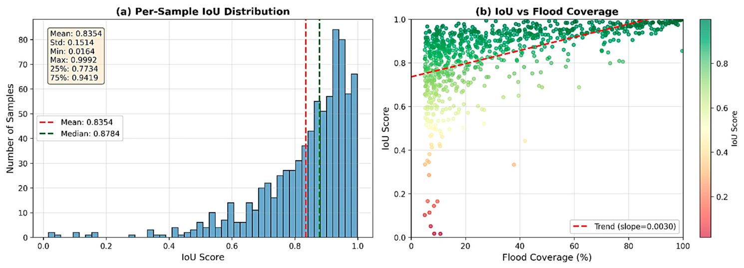
The per-sample IoU distribution shows that the model performs consistently well across most test cases, with IoU values heavily concentrated above 0.80 and a median (0.8784) exceeding the mean (0.8354), indicating generally high-quality predictions with a small number of low-performing outliers (Figure 4a). These outliers likely correspond to challenging scenes with limited or fragmented flood regions. The IoU–flood-coverage analysis further reveals a weak positive correlation, suggesting that samples with larger flood extents tend to yield slightly higher accuracy due to clearer spatial patterns and stronger contextual cues, while lower IoU scores occur primarily in images with minimal flood coverage, where small misclassifications disproportionately affect performance (Figure 4b). Overall, the results demonstrate robust segmentation across diverse conditions, with performance reductions mainly associated with small, difficult-to-detect flooded areas.

4.2. Training Dynamics

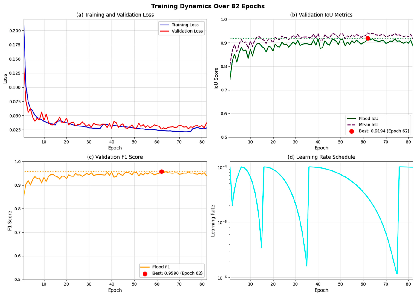
Training proceeded for 82 epochs before early stopping was triggered due to no more improvement in validation loss over 20 consecutive epochs. The best model, selected based on minimum validation loss, was obtained at epoch 62. The total training time was approximately four hours on the specified hardware.

The validation IoU metrics show steady improvement, with both flood IoU and mean IoU stabilizing above 0.90 and reaching their peak around epoch 62, indicating strong generalization to unseen data. Similarly, the validation F1-score follows an upward trend before plateauing near 0.95, reinforcing the model’s consistent performance across epochs. The cosine annealing learning rate schedule with warm restarts provided periodic increases in learning rate, which appeared to facilitate escape from suboptimal local minima and contributed to the stable convergence behavior observed during training. The training and validation curves are presented in Figure 5.

4.3. Comparison with State-of-the-Art Methods

Table 7. Comparison with state-of-the-art methods on the S1GFloods dataset.

Method	Architecture	OA (%)	Precision (%)	Recall (%)	F1 (%)	IoU (%)
DAM-Net [14]	Vision Transformer	97.8	97.4	95.6	96.5	93.2
Proposed Method	CNN + Attention	97.37	94.55	97.64	96.07	92.43
Siam-NestedUNet	CNN	97.2	95.1	95.7	95.4	92.7
BIT	Vision Transformer	97.7	97.7	93.8	95.7	92.2
SNUNet-CD	CNN	97.0	95.5	93.1	94.3	90.5
SwinSUNet	Vision Transformer	97.1	96.8	92.5	94.6	89.8
DTCDSCN	CNN	96.4	95.6	92.1	93.8	88.3
FC-Siam-Conc [21]	CNN	96.8	96.3	91.2	93.7	88.1
FC-Siam-Diff [21]	CNN	94.9	94.5	90.0	92.2	85.4

introduces a comparison of the proposed method with current approaches evaluated on S1GFloods dataset. The benchmark results for comparison methods are reproduced from Saleh et al. [14].

The proposed method achieves the third-highest IoU among the compared methods, trailing DAM-Net by 0.77% and Siam-NestedUNet by 0.27%. However, the proposed method achieves the highest recall (97.64%) among all methods, exceeding DAM-Net by 2.04 percentage points. This suggests that the proposed approach may be particularly effective at minimizing missed detections, albeit with a slightly higher false positive rate.

4.4. Model Complexity Analysis

Table 8. Model complexity comparison.

Method	Architecture	Params (M)	FLOPs (G)
DAM-Net	ViT	19.5	32.0
Proposed	CNN + Attention	34.0	32.7
BIT	ViT	24.4	25.2
SwinSUNet	ViT	28.2	31.3
DTCDSCN	CNN	31.3	26.4
SNUNet-CD	CNN	12.0	109.6
FC-Siam-Conc	CNN	1.5	10.6

compares the model complexity of different approaches. The proposed method contains 34.0 million parameters, which is larger than DAM-Net (19.5M) but comparable to other CNN-based methods. The increased parameter count is primarily attributable to the ResNet34 encoder, which provides robust feature extraction at the cost of additional parameters.

In addition to parameter count and FLOPs, we measured wall-clock inference time on an NVIDIA A100-SXM4-40GB GPU with FP16 mixed precision. Averaged over 1000 forward passes (after 50 warm-up runs) at 256 × 256 input resolution, the proposed model achieves a per-image latency of 15.34 ± 1.09 ms when processing a single image (throughput ≈ 65 images/sec) and 1.33 ms per image when processing batches of 16 (throughput ≈ 755 images/sec). These figures indicate that the model is well within the budget required for real-time operational flood mapping pipelines: a single Sentinel-1 IW scene tiled into 256 × 256 patches at 10 m resolution can be processed in under one minute on a single A100, even in the single-image (batch = 1) regime.

4.5. Ablation Study on Fusion Strategy

To isolate the contribution of the Differential Attention module, we trained two ablation variants from scratch on the S1GFloods training split using identical hyperparameters (encoder: ResNet34 ImageNet-pretrained; loss: 0.5 × Dice + 0.5 × Focal; optimizer: AdamW, lr = 1 × 10⁻⁴; up to 50 epochs with patience = 15) and evaluated all three on the same test split (

Table 9. Fusion strategy ablation on S1GFloods Test Set (805 samples). All variants share the same ResNet34 Siamese encoder, U-Net decoder, training loss, and optimizer; only the per-scale fusion module differs.

Variant	Fusion	IoU (%)	F1 (%)	Precision (%)	Recall (%)	Params (M)
A	Concat (no diff, no attn)	91.68	95.66	93.38	98.05	25.14
B	Diff-only (no attn)	90.48	95.00	94.96	95.04	24.44
C	Diff + Attention (proposed)	92.43	96.07	94.55	97.64	33.95

): (i) Variant A—Concatenation, where pre and post features are concatenated and reduced to C channels via a 1 × 1 convolution (no explicit difference, no attention); (ii) Variant B—Pure difference, using the absolute element-wise difference |F_post − F_pre| with no attention; and (iii) Variant C—Differential Attention (proposed), as described in Section 3.2.

The results in Table 9 reveal a non-monotonic relationship between the three variants. Variant B (90.48% flood IoU) underperforms the simpler Variant A (91.68% flood IoU) by 1.20 percentage points, indicating that the absolute difference operation alone discards absolute backscatter information that is informative for distinguishing flood-induced water from permanent dark surfaces (e.g., asphalt, terrain shadows, or seasonally bare soil). The proposed Differential Attention (Variant C, 92.43% flood IoU) compensates for this information loss by re-incorporating the post-flood features through the attention pathway σ(Conv([F_post, D])), yielding +1.95 pp flood IoU over Variant B and +0.75 pp over Variant A. This empirically validates each architectural choice: the difference operation provides the temporal change signal, while the attention mechanism is essential for preserving the absolute backscatter context that the bare differencing destroys. Notably, the simple Concat baseline (Variant A) already achieves competitive performance (95.66% F1, 98.05% recall) at lower parameter cost (25.14M vs. 33.95M), suggesting it as a useful lightweight alternative when computational resources are constrained.

4.6. Error Analysis

Based on the precision–recall balance, the error characteristics of the proposed method can be characterized as shown in

Table 10. Error analysis with potential causes.

Error Type	Rate	Potential Causes
False Negatives	2.36%	Partial flooding, mixed pixels at boundaries, wind-roughened water
False Positives	5.45%	Shadow regions, smooth nonwater surfaces, seasonal vegetation changes

.

The higher false positive rate compared to false negative rate indicates that the model is biased toward detecting potential flood areas. This bias is consistent with the high recall achieved and may be desirable for disaster-response applications where missing flooded areas carries higher cost than false alarms.

4.7. Qualitative Analysis

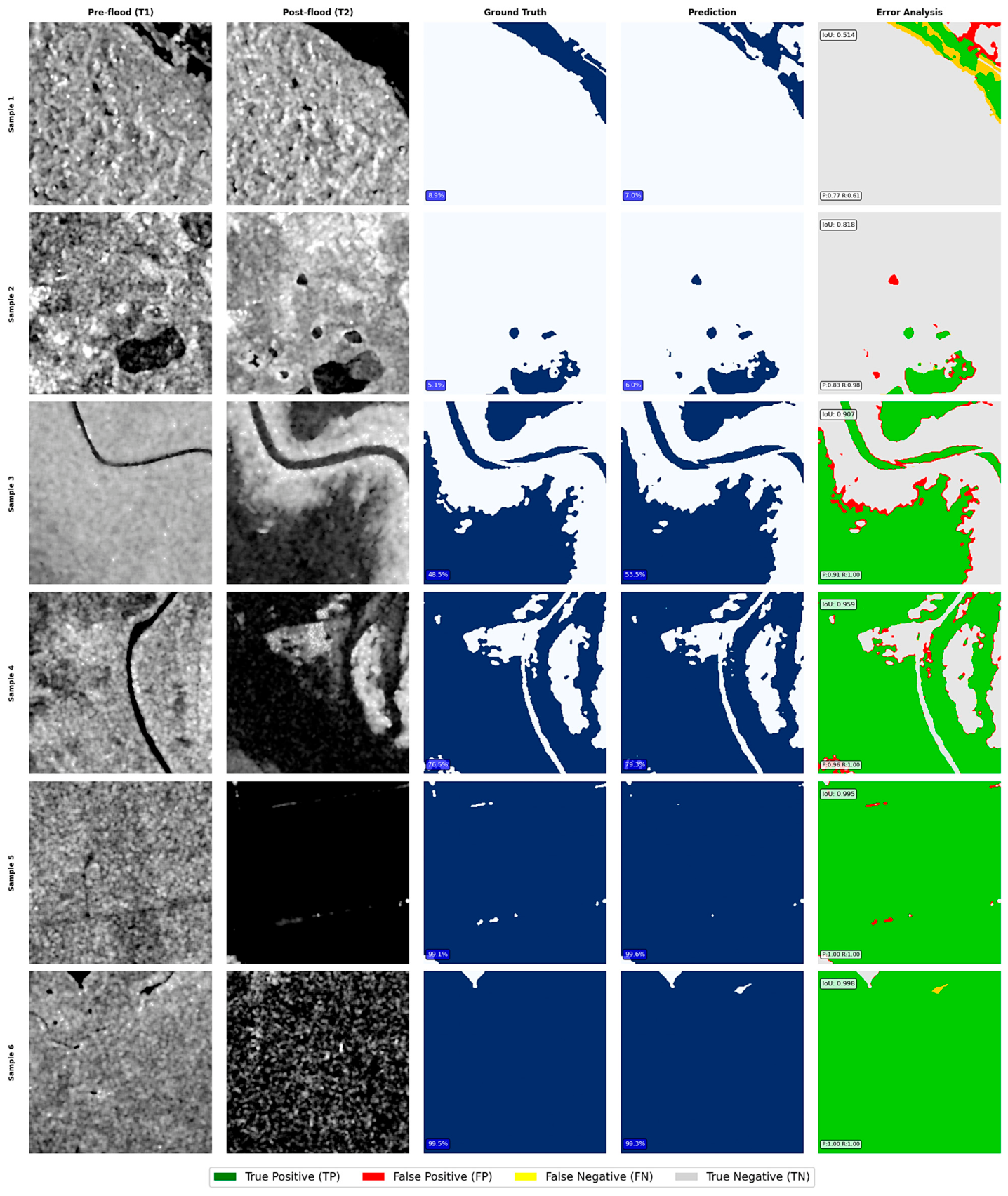
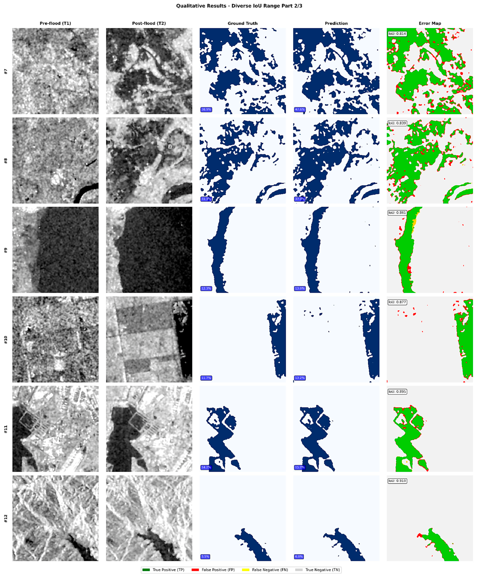
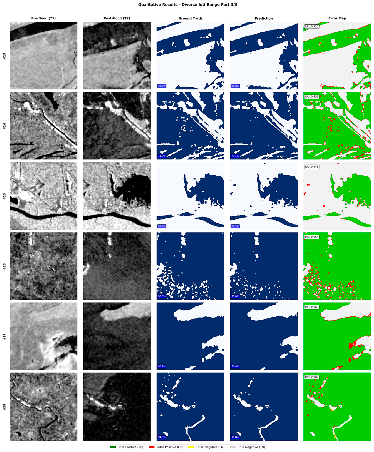
Qualitative segmentations for test examples in Figure 6 are compared to ground-truth, and visually demonstrate that the proposed model can effectively and accurately identify and delineate flood boundaries under various conditions.

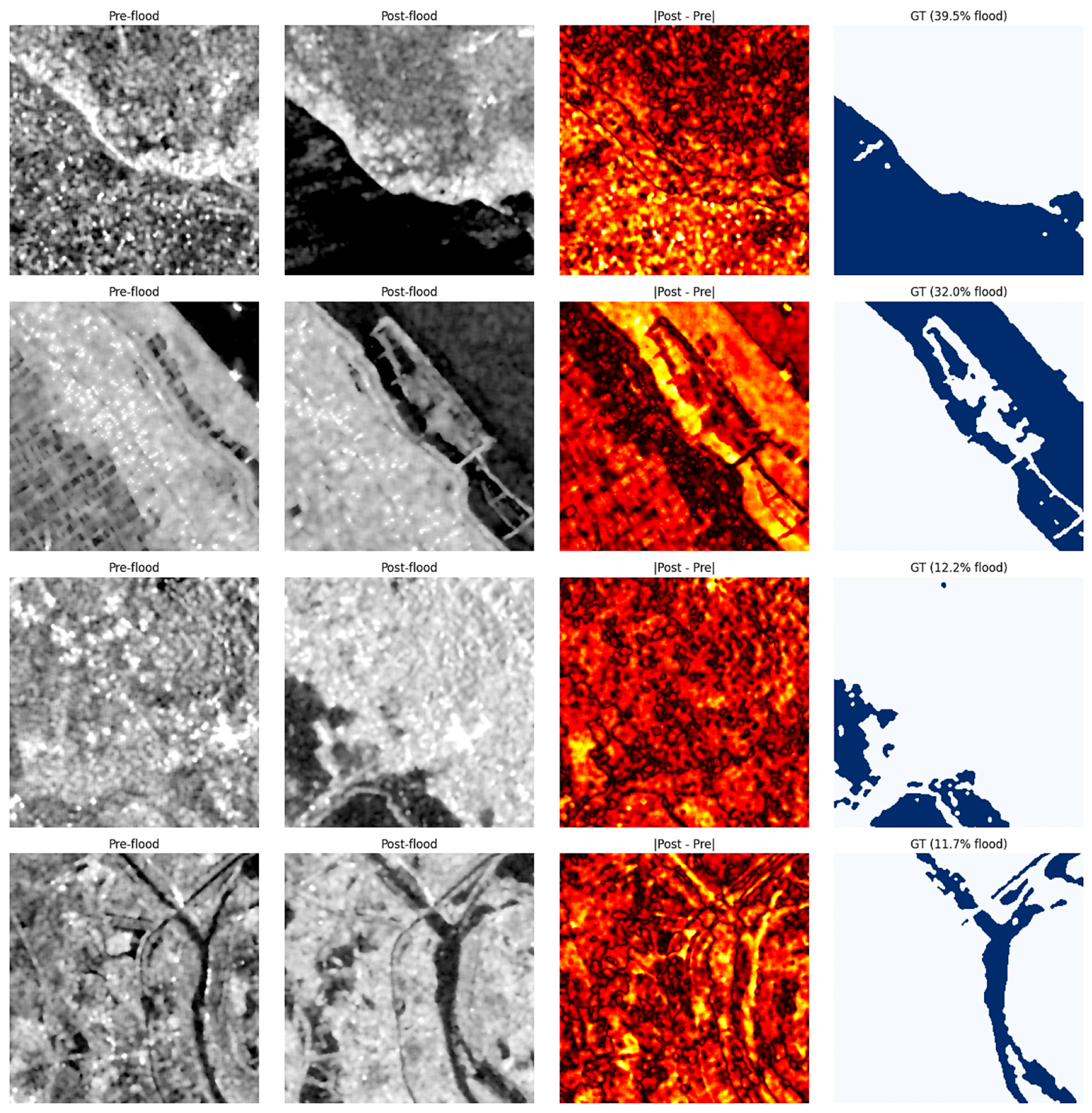
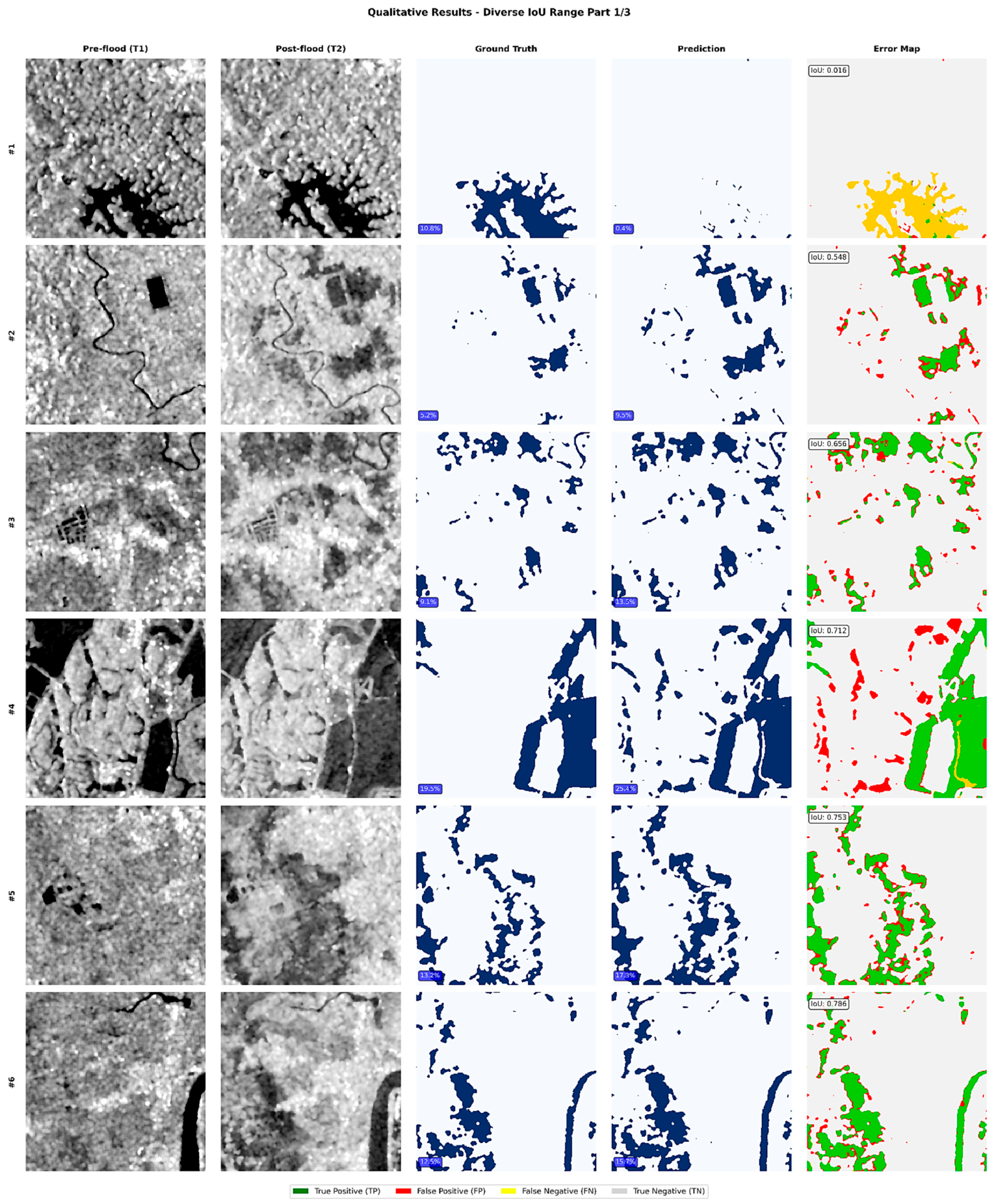
Additional qualitative results are presented in Figure A1 for non-standard water bodies and dense vegetation areas, in Figure A2 for urbanized regions, and in Figure A3 for man-made and fine-scale water structures.

4.8. Large-Scale Operational Demonstration

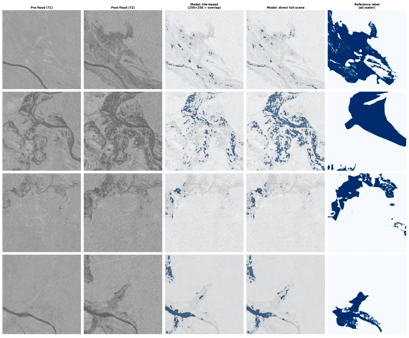
To demonstrate the model’s capacity for large-scale operational deployment beyond the 256 × 256 training tile size, we evaluated the proposed Siamese U-Net on full-resolution 512 × 512 bi-temporal Sentinel-1 chips drawn from the Sen1Floods11_Modified dataset covering Ghana flood events with 10–37% flood coverage. Because the architecture is fully convolutional, the model accepts arbitrary spatial input sizes that are multiples of 32; we therefore compared two inference modes: (i) direct full-scene inference at the native 512 × 512 resolution, and (ii) tile-based inference using overlapping 256 × 256 windows with 64-pixel overlap and Hann-window blending in the overlap regions. Figure 7 visualizes both modes alongside the pre-flood and post-flood SAR images and the reference label. The two inference modes produce visually consistent flood maps, confirming that operational deployment on arbitrarily large Sentinel-1 scenes is feasible through tile-based processing. Combined with the inference latency reported in Section 4.4, a complete Sentinel-1 IW scene (e.g., 25,000 × 16,500 pixels) can be processed via tile-based inference in under five minutes on a single A100 GPU, making the proposed pipeline suitable for near-real-time operational flood mapping.

5. Discussion

5.1. Limitations

The potential limitations of the proposed research are provided below:

(1) Data Split Methodology: Like both studies and the previous evaluation of DAM-Net, the use of partitioning strategies for samples from the same flood event results in the possibility that some samples from the same flood event could be found in multiple partitions (e.g., training, validation, testing). This is an issue, as described by Bountos et al. [16], with SAR flood detection datasets such as S1GFloods as the use of this method causes spatial autocorrelation between samples from the same geographic area and samples from the same satellite pass to be included in both training and testing. Using geographic splitting based on flood event would have provided better separation between the training and testing of the models and improved evaluation of their ability to generalize to completely unseen events and areas.

(2) Urban Flood Detection: In urban environments, double-bounce scattering leads to flooded zones appearing brighter than they were before flooding occurred, which is contrary to the general assumption of “dark water” that most SAR-based flood-detection algorithms use [10]. The attention mechanism may help with learning a weighting that can partially account for this; however, explicit treatment of urban flooding was not implemented into this model.

(3) Splitting Border Challenge: Although it was identified in the study conducted by Saleh et al. [14] that the division of very large satellite images into fixed size patches could create ambiguities in scenarios when the boundary of a flood falls on the edge of an image patch, this ambiguity creates a potential degradation in the ability to detect floods. This limitation is inherent in all patch-based methods and will be a major limitation for the use of satellite data for operational flood mapping.

(4) Polarization Utilization: In addition to using the current method to replicate the single channel intensity image across the three input channels, as opposed to utilizing the complementary information found within the VV and VH polarizations, the use of a polarimetric method would provide for better separation between flooded vegetative areas and flooded urban areas [26].

5.2. Future Work

The future research can be directed towards following aspects:

(1) Event Based Split Evaluation: In accordance with the S1GFloods benchmark, a random partition was used in the present research to provide a fair basis for the comparison of results; however, the use of such a methodology can result in patches of the same flood being included in both the training and testing data which can create spatial autocorrelation, as noted by Bountos et al. [16]. A future line of research will include using an event-based geographic splitting strategy (leave-one-flood-out), which would allow for testing of the model on completely unseen flood events and allow for better assessment of the model’s ability to generalize in realistic applications.

(2) Multi-Sensor Fusion: The fusion of SAR Sentinel-1 (synthetic aperture radar) data with Sentinel-2 optical data can be used to enhance the quality of flood mapping by providing additional spectral information in cases of a clear sky (cloud-free) [27]. This is especially true in difficult environments (e.g., flooded vegetation or urban environment) in which SAR-based techniques have difficulty due to inherent limitations of the technique.

(3) Large-Scale Mapping Validation: Large-scale flood inundation mapping applications (such as those illustrated by the Nebraska and Iran examples in the S1GFloods dataset and where reference F1-scores were reported to be 89.3 percent and 87.2 percent, respectively [14]) will provide opportunities to evaluate the utility of the developed model for operational flood monitoring systems.

6. Conclusions

In this research, a Siamese U-Net architecture that incorporates Differential Attention for flood extent mapping using SAR has been presented. Our method was tested on the S1GFloods dataset, yielding a flood IoU of 92.43%, an F1-Score of 96.07%, and a recall of 97.64%. The proposed method’s results are comparable to other top performing methods, as they were only 0.77% less than the DAM-Net benchmark. Additionally, it utilizes a more basic architecture (a CNN encoder) compared to the Vision Transformer used as the backbone for the DAM-Net. The proposed method’s high recall demonstrates its ability to perform well in disaster-response scenarios, in which detecting all flooded regions is emphasized. The Differential Attention mechanism allows for an interpretive way to detect the bi-temporal change due to flooding by emphasizing the flood-induced changes and suppressing both noise- and pseudo-changes. Overall, the reported metrics highlight that the model performs reliably in identifying flood extent, with strong generalization across classes and a favorable precision–recall balance. These results indicate that the segmentation approach is well-suited for practical deployment in flood monitoring and rapid damage assessment workflows.