Fast Firefighting Water Capacity Assessment Using a Streamlined Single-Loop Hybrid Search ^†

Abstract

The water distribution system firefighting capacity is widely estimated using decades-old methods that are inefficient for the scale of typical models nowadays. This article introduces an updated algorithm that streamlines the estimation by using a single iterative loop that simultaneously solves for hydrant capacity and the hydraulic effects on the network. The method features a hybrid physically based and heuristic local search approach, and a strategy to easily rank the criticality of network elements that might violate service level constraints. Tests on three models of varying size demonstrate the significant accuracy and efficiency benefits of the proposed approach.

1. Introduction

Water distribution systems should possess sufficient spare capacity for firefighting eventualities. Regulations in several countries thus require that each hydrant can provide sufficient flow while maintaining the regular operating service pressure level throughout the system [1]. Although determining this capacity for individual hydrants is relatively straightforward, large utilities struggle to efficiently conduct systemwide assessments because of the complexity of their networks and the numerous hydrants to be considered.

Existing simulation engines utilize iterative methods developed decades ago to perform these types of assessments [2]. However, these are often inefficient in ways that become apparent with complex networks. First, they need to sequentially search for a “critical element”, i.e., the junction whose low pressure or the pipe whose high velocity might first violate the established limits if the estimated demand were to increase. Second, they deploy different search algorithms of varying levels of efficiency depending on whether velocity constraints in pipes should be considered in addition to pressure constraints in junctions. Together, these limitations have led to methods involving multiple nested loops with computational times of several hours (or even days) for a single proposed configuration of a complex network. This article thus introduces an algorithm for quickly determining the capacity of single hydrants by streamlining these steps, previously bottlenecks, into a single agile loop.

2. Methods

Fire flow analyses typically comprise the following three levels of firefighting demand at each hydrant: the “required”, “available”, and “design” flow. The required demand is that which is expected to be sufficient to extinguish fires given the built or planned infrastructure. The available flow is the maximum that can be extracted with at least a minimum pressure at the hydrant, notwithstanding the impact on the network. The design flow is the maximum available without violating service-level constraints in the network. The three levels, and their impact on the system’s hydraulic behavior, are all important in planning and operational firefighting decision-making processes [3].

Assuming a steady-state operation scenario, computing the required and available demands and their impact on the network can be performed with a single hydraulic run each, e.g., using the Global Gradient Algorithm (GGA) [4]. On the other hand, computing the design flow has traditionally been carried out by iteratively solving the network hydraulics multiple times. This is mostly due to the uncertainty of which junction or pipe will ultimately be the one that limits the flow before violating its constraint—the “critical” element. Taking the traditional InfoWater solver as an example (one of the most used in the industry), there is a three-level loop [5] as follows: (1) An outer loop that iterates over potential critical elements, (2) an intermediate loop that iterates over guesses for the design flow value, and (3) an inner hydraulic loop that evaluates the impact.

The method proposed here is based on the GGA implementation in EPANET [6], and it expands upon some of its constituting steps to simultaneously find, in a single loop, solutions for the selection of the critical element j, the design flow Q, and the resulting hydraulic impact. The steps are performed at each iteration of the loop until convergence is achieved or a maximum iteration count is reached. Figure 1 summarizes the original steps [7] and the modifications introduced here.

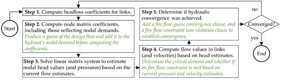
Figure 1. Step loop with proposed modifications in italics.

Once the loop exits, the last guess for the design flow Q produced in Step 2 is returned. The next subsections present the details of the modifications in steps 2, 4, and 5.

2.1. Producing Design Fire Flow Guesses

As a preliminary part of Step 2 in the GGA, the design fire flow demand guess Q is produced by a two-layer strategy, with a preferred physically based layer that is faster and generally more accurate, and a back-up heuristic layer in case the first one fails.

2.1.1. Physically Based Design Fire Flow Guess

A Cholesky decomposition [8] creates a quadratic regression model for the design fire flow demand Q in terms of the critical variable x as follows:

$$Q=c_1{x}^2+c_{2}x+c_3,$$

(1)

based on the three last guesses for $Q$ and their corresponding values for $x$. $x$ is pressure if the critical element is a junction or velocity if it is a pipe. Before the first iteration, the previous guesses are initialized with those from the static demand, required flow, and available flow conditions. The new guess for $Q$ is computed by plugging into this model a value of $x$ equal to the violation threshold $x^{*}$. While simpler regression training methods can be used, using Cholesky allows for higher-degree polynomials, although the second degree is concordant with observations [2].

2.1.2. Heuristic Back-Up Design Fire Flow Guess

${∆}_i=Q_i-Q_{i-1}$ is the change in $Q$ between the current iteration $i$ and the previous one $i-1$. $d_i\in \{+,-\}$ is the direction of ${∆}_i$. The guess produced with Equation (1) is expected to be smaller than the previous one ($d_i=-$) if at least one constraint was violated in the previous iteration $i-1$ (see Section 2.2) or larger ($d_i=+$) if none were. However, given the inexact intermediate estimates of $x$ before hydraulic convergence is achieved, that guess might not be in the desired direction of change. This can also be a consequence of non-typical hydraulic behavior in the presence of pumps and valves, where the parabolic assumption in Equation (1) might not (locally) hold. In such a case, a heuristic local search overrides the physically based guess by modifying the previous guess $Q_{i-1}$ as follows:

$$Q_i=Q_{i-1}+m_i·{∆}_{i-1},\mathrm{w}\mathrm{h}\mathrm{e}\mathrm{r}\mathrm{e}{m}_i=\left\{\begin{array}{cc}1.1& \mathrm{i}\mathrm{f}{d}_i=d_{i-1}\\ -0.4& \mathrm{o}\mathrm{t}\mathrm{h}\mathrm{e}\mathrm{r}\mathrm{w}\mathrm{i}\mathrm{s}\mathrm{e}\end{array}\right.$$

(2)

This update guarantees the new guess $Q_i$ is in the correct direction. The values for the multiplier $m$ were tuned through trial-and-error to expand the change rate (1.1) when subsequent guesses have fallen short, and to contract it (−0.4) when the target is overshot. While this heuristic local search is less elegant than something like binary search (or “bisection”), it does not require knowing the bounds of the design fire flow $Q$ beforehand.

2.2. Selecting the Critical Element and Evaluating Constraint Violation

The critical element is usually the junction whose pressure violation is the largest in the simulation with the available fire flow; however, how should we compare the pressure violations with the velocity violations when the latter are included? Or how do we account for cases where the controls make the system’s response non-continuous and/or non-monotonous thus potentially “shifting” element criticality away? Here, we propose ranking criticality after the pressures and the velocities are known at the end of Step 4, by using the “relative closeness” $r_j$ of the variable $x_j$ of each potential critical element $j$ to their corresponding threshold $x_j^{*}$. $r_j$ is the ratio of the difference between $x_j$ and $x_j^{*}$, and the range of variation in $x_j$ in the static, required, and available flow runs. $r_j$ is negative when there is a violation and positive when there is none. The critical element $j_{\mathrm{c}\mathrm{r}\mathrm{i}\mathrm{t}}$ is thus chosen as the one with the smallest value of $r_j$, $j_{\mathrm{c}\mathrm{r}\mathrm{i}\mathrm{t}}=\arg {\mathrm{m}\mathrm{i}\mathrm{n}}_j{r}_j$. This normalized metric not only allows us to fairly compare junctions and pipes but also elements with wildly different variation ranges.

2.3. Determining Convergence

Aside from the regular criteria used to establish convergence in Step 5 of the GGA loop, here, we introduce two additional checks that must be satisfied. The first one is that no constraints are violated, that is $r_{j_{\mathrm{c}\mathrm{r}\mathrm{i}\mathrm{t}}}\ge 0$. The second one is that the change in the last two design flow guesses is smaller than a user-defined precision value $\epsilon$; that is $\left|{∆}_i\right|<\epsilon$.

3. Experimental Setup and Results

We implemented the proposed algorithm in C++ within InfoWater Pro [5]. To test its accuracy, we used a playground water distribution model, “Small”, and two real-world ones, “Medium” and “Large”. For each, we ran an analysis with only pressure constraints, and another with velocity constraints added. To determine the accuracy of the obtained design fire flow, we compared the threshold value $x_{j_{\mathrm{c}\mathrm{r}\mathrm{i}\mathrm{t}}}^{*}$ with the modeled critical value $x_{j_{\mathrm{c}\mathrm{r}\mathrm{i}\mathrm{t}}}$ when the fire demand was applied; they are ideally equal. Table 1 summarizes the characteristics of the three models (number of pipes, number of hydrants analyzed, and average demand), and the results obtained using the legacy and the proposed algorithms. The results shown are the mean absolute error (MAE) of $x_{j_{\mathrm{c}\mathrm{r}\mathrm{i}\mathrm{t}}}$ across all hydrants, and the MAE relative to $x_{j_{\mathrm{c}\mathrm{r}\mathrm{i}\mathrm{t}}}^{*}$ (RMAE). We also list the number of hydrants for which the flow was limited by pressure and not by velocity, and the number of hydrants where the critical element was different (shifted) from that of the available flow condition.

Table 1. Characteristics of the three test models and results using legacy and proposed algorithms.

	Small	Medium	Large
Pipes|hydrants|average demand (L/s)	58|30|3.66	2092|1638|790	151,597|200|12,650
Pressure MAE: legacy|proposed	0.01587|0.00141 (psi)	0.00082|0.00031 (mwc)	0.02269|0.00931 (psi)
Pressure RMAE: legacy|proposed	0.0794%|0.0070%	0.0041%|0.0015%	0.1135%|0.0466%
Critical element shift	0	73	3
Press. and vel. RMAE: legacy|proposed	0.2240%|0.0011%	0.0730%|0.0008%	0.2031%|0.0697%
Pressure-limited hydrants|crit. shift	18|1	1004|47	30|0

To test the performance, we analyzed 51 hydrants in the Large model, with ten replicated runs in which we measured the time it took to determine the design fire flow in an Intel Core i7-11850H CPU with 32 GB RAM. With pressure constraints only, it took an average of 6.12 s with the legacy algorithm and 6.18 with the proposed one. With both pressure and velocity constraints, it took 48.51 (legacy) and 15.28 s (proposed).

4. Conclusions

The tests showed that the proposed single-loop hybrid search algorithm significantly improved the accuracy of design fire flow estimations in models of different sizes. Errors were reduced to 41% in the worst-case scenario and down to 0.5% in the best-case scenario compared to those of the legacy InfoWater algorithm. The largest reductions occurred in analyses with both pressure and velocity constraints. While the performance test in the Large model did not show benefits when only pressure constraints were considered, the proposed method displayed a significant speed-up of 3.17 when adding the velocity constraints. Additionally, while not very common, the occasional shifting of the critical element also validated the need to simultaneously consider all the potential critical elements in the analysis. The algorithm was released publicly in version 2024.3 of InfoWater Pro.

References

- American Water Works Association. Distribution System Requirements for Fire Protection; American Water Works Association: Washington, DC, USA, 2008. [Google Scholar]
- Boulos, P.F.; Rossman, L.A.; Orr, C.H.; Heath, J.E.; Meyer, M.S. Fire Flow Computation with Network Models. J. Am. Water Works Assoc. 1997, 89, 51–56. [Google Scholar] [CrossRef]
- Kanta, L.; Zechman, E.; Brumbelow, K. Multiobjective Evolutionary Computation Approach for Redesigning Water Distribution Systems to Provide Fire Flows. J. Water Resour. Plan. Manag. 2012, 138, 144–152. [Google Scholar] [CrossRef]
- Todini, E.; Pilati, S. A Gradient Algorithm for the Analysis of Pipe Networks. In Computer Applications in Water Supply: Volume 1—Systems Analysis and Simulation; Research Studies Press Ltd.: Baldock, UK, 1988; pp. 1–20. [Google Scholar]
- Autodesk Inc. InfoWater Pro Documentation. Available online: https://help.autodesk.com/view/INFWP/ENU/ (accessed on 3 September 2024).
- Rossman, L.A.; Woo, H.; Tryby, M.; Shang, F.; Janke, R.; Haxton, T. EPANET 2.2 User Manual; Water Infrastructure Division, Center for Environmental Solutions and Emergency Response, US Environmental Protection Agency: Cincinnati, OH, USA, 2020.
- EPANET Hydraulic Solver Source Code. Available online: https://github.com/OpenWaterAnalytics/EPANET/blob/dev/src/hydsolver.c (accessed on 3 September 2024).
- Hernández, F.; Liang, X. Hybridizing Bayesian and Variational Data Assimilation for High-Resolution Hydrologic Forecasting. Hydrol. Earth Syst. Sci. 2018, 22, 5759–5779. [Google Scholar] [CrossRef]
Disclaimer/Publisher’s Note: The statements, opinions and data contained in all publications are solely those of the individual author(s) and contributor(s) and not of MDPI and/or the editor(s). MDPI and/or the editor(s) disclaim responsibility for any injury to people or property resulting from any ideas, methods, instructions or products referred to in the content. |
© 2024 by the author. Licensee MDPI, Basel, Switzerland. This article is an open access article distributed under the terms and conditions of the Creative Commons Attribution (CC BY) license (https://creativecommons.org/licenses/by/4.0/).