Abstract
Periodic series of period T can be mapped into the set of permutations of . These permutations of period T can be classified according to the relative ordering of their elements by the horizontal visibility map. We prove that the number of horizontal visibility classes for each period T coincides with the number of triangulations of the polygon of vertices that, as is well known, is the Catalan number . We also study the robustness against Gaussian noise of the permutation patterns for each period and show that there are periodic permutations that better resist the increase of the variance of the noise.
1. Introduction
Periodic or noisy periodic time series appear in many natural phenomena. Strictly speaking, real signals are approximately periodic and are considered to incorporate a certain seasonality [1,2]. They can also be solutions of dynamical systems, either discrete or continuous [3,4]. In practice, periodicity is finite, that is, it appears in a finite set of points. However, theoretically, these periodic series extend to infinity and, thus, they allow the consideration of the limit of infinite periods. This paper is focused on the study of the complete set of periodic natural series for each period . Indeed, there are other classical approaches, such as, for instance, the Fourier analysis, that provide a complete set of solutions to this problem. However, our approach does not pretend to surpass them but, on the contrary, to offer an alternative viewpoint for studying this kind of time series.
A discrete series , infinite or not, is said to be periodic if there is a natural number T such that for all , that is, after a transient period . For real valued series , there are infinite periodic series for each period T (see Figure 1 for an example). However, this infinite number of cases can be reduced to a finite number by means of the application of discrete mappings, such as the horizontal visibility map [5]. It is worth pointing out that, for the horizontal visibility map, the time scale is not relevant, since only the values of any pair of points are compared. This means that the same horizontal visibility pattern is obtained if the time units are either seconds or years or, in the case of spatial series, either millimeters or kilometers.
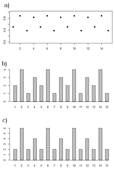
Figure 1.
(a) is a real-valued time series obtained from the logistic map with initial condition , after a transient period of time steps. The growth rate value is: , which corresponds to a period 4 solution. (b) is the corresponding permutation set obtained by ranking the values of the real-valued series. (c) The associated horizontal visibility pattern is: .
2. Permutations of Periodic Series and Their Horizontal Visibility Patterns
A real valued periodic time series can be mapped into a positive integer series in which the elements within the period are ranked according to their value. For instance, as shown in Figure 1, a period 4 series with real values:
obtained from the logistic equation, , , is mapped into the positive integer series: . Thus, any real valued time series can be transformed using this method. Let us assume that the largest value is fixed as the first value in each period. Then, if no equal values occur within the period, there are possible permutations for the period T. Formally, given a periodic series of period T, we define its permutation pattern as the natural numbers that rank the values within the period, starting from the largest, that takes the value T. It is worth noting that all of these permutation patterns are effectively generated by applying the generic function Rank, a command that is defined in most programming languages.
All periodic patterns can be obtained as permutations of the set and studied by applying combinatorial techniques [6,7]. In this context, the question is how these permutation patterns can be classified with regards to a definite order, for example, that turns out from the horizontal visibility map [5].
Two points of the series, and with , are said to see each other horizontally if
Since the horizontal visibility algorithm is only dependent on the relative values between the points of the integer series, it turns out that different permutation patterns could be classified within the same category. Indeed, the application of the horizontal visibility map enables a substantial reduction of the set of all permutation patterns.
In practice, for any permutation pattern, we can obtain the associated horizontal visibility pattern: for each value of the series, we calculate the ordinal of its horizontal visibility basin, that is, the number of points that are horizontally seen from the said value, for example, as shown in Figure 1, the horizontal visibility pattern of the permutation is . This means that the largest value has six points in its visibility basin and the remaining points, 1,3,2 have two, four and two points, respectively, in their visibility basins.
In order to count the number of horizontal visibility patterns that exist for each permutation pattern of period T, it is convenient to represent the values of the period as a convex polygon of vertices. To each vertex of this polygon, we assign the corresponding value of the element of the series and read counterclockwise (see Figure 2). If we link the vertices forming the corresponding horizontal visibility graph, the projection of the edges forms a triangulation of the polygon. If we map each of the permutations into a polygon and compute their triangulation, we obtain all of the possible triangulations of these polygons of vertices. For example, Figure 3 depicts the six polygons that appear for period . Please note that the label 4 appears twice, in order to close the period.
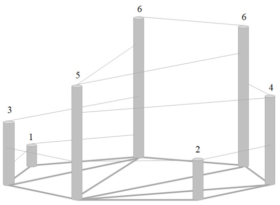
Figure 2.
Tridimensional representation of a labeled heptagon that corresponds to the permutation pattern of period : . Its horizontal visibility pattern is obtained summing all the edges of the vertices, counting both 6-vertices. The projection of the horizontal visibility links on the plane yields the triangulation.
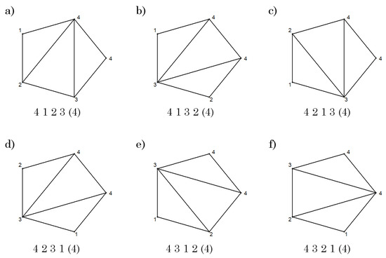
Figure 3.
The six polygon triangulations related to the six possible permutation patterns for the period time series. As can be observed, triangulations (b,d) are equal and correspond to the same horizontal visibility pattern. On the other hand, the other four triangulations (a,c,e,f) have a unique correspondence (see Table 1).
The triangulation of convex polygons is a classical problem and it is well known that, for a polygon of vertices, the number of possible triangulations is given by the Catalan number :
This means that the infinite real valued series of period T can be reduced to horizontal visibility patterns. Nonetheless, even after this reduction, the number of horizontal visibility patterns increase exponentially with the period:
For example, for a period , the number of possible horizontal visibility patterns rises to .
A property that can be immediately deduced from the polygon triangulations is that the total visibility, , of any horizontal visibility pattern is the same for each period [8]: it is the sum of the edges that appear in the triangulated polygon multiplied by 2:
It can also be proven that, for each period T, the maximum visibility that any permutation pattern can attain is . In addition, the other permutation patterns reach other maxima: (see Table 2). For instance, for , there are four permutations with the largest visibility and two permutation patterns with a maximum visibility of 5. Note that the maximum visibility might not occur for the largest value. For instance, the permutation pattern corresponds to the horizontal visibility pattern: .

Table 2.
Number of maximal visibilities for low period series.
Another property that is worth mentioning is the average visibility of a point for each period, [9]. It is obtained from the total visibility of each period divided by the period:
Evidently, it tends to four as T tends to infinity.
The correspondence between permutation patterns and horizontal visibility patterns is not evident, as shown in Table 3. Columns provide the relation between permutations and horizontal visibility pattens. The first column indicates the number of permutations that are related univocally to a visibility pattern for each period T (rows). Similarly, the entries of the second column provide the number of permutations that are related to two visibility patterns for each period T, and so on. This table forms a reduced schelon matrix with some internal patterns that deserve to be commented on briefly. The entries of the first column grow as , whereas for the second column, they grow as . For the first three rows, the number of columns with non null entries are 2, 3 and 6. Surprisingly, there are some columns, for example, 7 and 9, which appear for the first time at period and , respectively. Unfortunately, the table is not complete, so no rigorous conclusions can be drawn for a larger order of columns and rows.
Table 3.
Each entry indicates the number of permutations for period T that corresponds to the number of visibility patterns. For instance, for period , there are eight permutation patterns related one-to-one to one visibility pattern. The other two appear each from two permutations and four come from three different permutations (see Table 1). The sum of each row yields the total number of visibility patterns for each period. The total permutation patterns for each period are obtained from each row, multiplying the entry by the value of each column. For example, the sum of the entries of the second row, for , gives the Catalan number and the weighted sum () equals the number of permutations .
Table 1 also shows the number of maxima (pinnacles) in the permutation patterns [6,10]. For these two periods , there are permutations that have no maximum, while others exhibit only one. The former permutations are related one-to-one to a horizontal visibility pattern. On the other hand, those permutations with one pinnacle can share the same horizontal visibility pattern. As a matter of fact, if the pinnacle takes the value of 3, for each horizontal visibility pattern there are two permutations, whereas if this value is 4, this correspondence is 3 to 1. Table 3 provides this equivalence for each period precisely.
Table 1.
The 6 and 24 permutation patterns for period and . These patterns correspond to 5 and 14 different horizontal visibility patterns. The number of interior pinnacles [6] and their values are shown in the fourth and the fifth columns.
3. Patterns of Noisy Periodic Series
As has been described in the previous section, for each period, more than one permutation is reduced to the same horizontal visibility pattern. The question is whether this equivalence remains when the signal is affected by any kind of noise, in particular Gaussian noise. It is expected that, when the intensity of the noise is small, the permutations of the noisy signal fall in the same visibility class as the non-perturbed time series and, consequently, all have the same horizontal visibility pattern. A similar problem has also been studied in [9]. Here, we focus on the problem of robustness against noise, for example, how Gaussian noise affects the permutation patterns as a function of the variance [11].
The way noisy series have been considered is detailed as follows:
(i) For each period T, we generate the synthetic permutations.
(ii) From each of these patterns, a series is generated.
(iii) To each of these series we add a random variable according to a normal distribution of null mean and standard deviation (specifically, the R-function [12]).
(iv) We vary the standard deviation from 0 to 6, with increments of 0.1. Consequently, 61 noisy series are generated from the initial permutation.
(v) The visibility algorithm is applied for all of the 61 series, including the periodic synthetic series.
(vi) To compare the noisy series with the periodic one, we count the number of coincidences between each pair of noisy-periodic series.
Figure 4 depicts the proportion of digit coincidences between the horizontal visibility patterns obtained from the noisy permutations as a function of the variance of the Gaussian noise for low periods. The same plot for each of the visibility patterns for period is presented in Figure 4. The proportion of coincidences is greater in both permutations, corresponding to the same visibility pattern: .
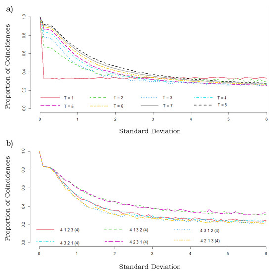
Figure 4.
(a) Proportion of coincidences (Y-axis) between the digits of the original series formed by repeated permutations and the noisy series that result after applying a Gaussian noise of standard deviation referred to in the X-axis. Please note that the level of coincidences achieved for large values of the standard deviation is compatible with a loss of memory, that is, the loss of any relationship with the original permutation as it is evident for period . (b) For , six visibility permutation patterns exist. When a time series formed by the repetition of each pattern is perturbed by a Gaussian noise with a standard deviation given in the X-axis, the proportion of coincidences with the original series decreases as shown in this figure. Note that the two series formed from the permutation patterns that correspond to the same horizontal visibility pattern: are more robust against white noise.
4. Concluding Remarks
Periodic or noisy periodic patterns appear in data sets from multiple fields of science [2]. In particular, a huge amount of data is formed by time series in which a unique variable, either discrete or continuous, is presented as a function of time that, indifferently, can also be considered discrete or continuous [3,4]. Many mathematical models also exhibit this oscillatory behavior and have been applied extensively to study its properties. Visibility algorithms are useful tools for the analysis of univariate series, for example, time series [13]. In particular, the horizontal visibility map provides analytical results about different types of series, namely periodic, random, fractional or chaotic [5]. Contrary to the natural visibility algorithm, the properties derived from the horizontal visibility map only depend on the ratio between the values of the points of the series, not on the distance between them. As shown in this paper, this enables a complete reduction of the infinite number of real valued periodic series to a finite set of visibility patterns. We prove that the number of horizontal visibility patterns for any period T is given by the Catalan number . Despite this huge reduction, the number of horizontal visibility patterns still grows exponentially as a function of T.
This exponential growth contrasts with the low number of visibility patterns that are found in the logistic map [14]. This is a consequence of the form of the field, , which sets the following rules of period doubling bifurcations:
- If previous values are such that , then the new duplicated values verify .
- The new points coming from and must be intercalated in time.
For instance, if these rules are applied to each period in the Feigenbaum cascade, a sequence of horizontal visibility patterns appears that, at the limit of the infinite period, converge to the ruler sequence [14,15]. Other unknown integer patterns are to be discovered in each of the infinite period doubling cascades that occur in the bifurcation diagram of the logistic and, in general, in unimodal maps.
Lastly, we would like to point out that it is also possible to obtain an elementary periodic pattern that corresponds to a given horizontal visibility pattern. The algorithm seeks to find a periodic pattern with the minimum positive integers that are compatible with the horizontal visibility map. Starting from the initial pattern , the program recurrently increases these values until the given horizontal visibility pattern is obtained. For example, for the horizontal visibility pattern , associated with permutation: , the elementary periodic pattern would be . It is important to remark that this relationship is one-to-one, that is, it is the unique elementary pattern that yields the given horizontal visibility pattern.
Institutional Review Board Statement
Not applicable.
Informed Consent Statement
Not applicable.
Data Availability Statement
Not applicable.
Conflicts of Interest
The authors declare no conflict of interest.
References
- Barnett, A.G.; Dobson, A.J. Analysing Seasonal Health Data; Springer: Berlin/Heidelberg, Germany, 2010. [Google Scholar]
- Franses, P.H.; Paap, R. Periodic Time Series Models; Oxford University Press: Oxford, UK, 2004. [Google Scholar]
- Galor, O. Discrete Dynamical Systems; Springer: Berlin/Heidelberg, Germany, 2007. [Google Scholar]
- Guckenheimer, J.; Holmes, P. Nonlinear Oscillations, Dynamical Systems, and Bifurcations of Vector Fields; Springer Science & Business Media: Berlin/Heidelberg, Germany, 2013. [Google Scholar]
- Luque, B.; Lacasa, L.; Ballesteros, F.; Luque, J. Horizontal visibility graphs: Exact results for random time series. Phys. Rev. E 2009, 80, 046103. [Google Scholar] [CrossRef] [PubMed] [Green Version]
- Davis, R.; Nelson, S.A.; Petersen, T.K.; Tenner, B.E. The pinnacle set of a permutation. Discret. Math. 2018, 341, 3249–3270. [Google Scholar] [CrossRef] [Green Version]
- Elizalde, S. A survey of consecutive patterns in permutations. In Recent Trends in Combinatorics; Beveridge, A., Griggs, J.R., Hogben, L., Musiker, G., Tetali, P., Eds.; The IMA Volumes in Mathematics and Its Applications 159; Springer International Publishing: Cham, Switzerland, 2016. [Google Scholar] [CrossRef] [Green Version]
- Nuño, J.C.; Muñoz, F.J. The partial visibility curve of the Feigenbaum cascade to chaos. Chaos Solitons Fractals 2020. [Google Scholar] [CrossRef] [Green Version]
- Núñez, A.; Lacasa, L.; Valero, E.; Gómez, J.; Luque, B. Detecting series periodicity with horizontal visibility graphs. Int. J. Bifurc. Chaos 2012, 22. [Google Scholar] [CrossRef] [Green Version]
- André, D. Étude sur les maxima, minima et séquences des permutations. In Annales Scientifiques de l’École Normale Supérieure. 3e série, Tome 1, pp. 121–134; Gauthier-Villars (Éditions scientifiques et médicales Elsevier): Paris, France, 1884. [Google Scholar]
- Amigó, J.M. Permutation Complexity in Dynamical Systems; Springer Series in Synergetics; Springer: Berlin/Heidelberg, Germany, 2010. [Google Scholar]
- Team RC. R: A Language and Environment for Statistical Computing; R Foundation for Statistical Computing: Vienna, Austria, 2018; Available online: https://www.R-project.org/ (accessed on 4 June 2021).
- Lacasa, L.; Luque, B.; Ballesteros, F.; Luque, J.; Nuño, J.C. From time series to complex networks: The visibility graph. Proc. Natl. Acad. Sci. USA 2008, 105, 4972–4975. [Google Scholar] [CrossRef] [PubMed] [Green Version]
- Nuño, J.C.; Muñoz, F.J. Universal visibility patterns of unimodal maps. Chaos 2020. [Google Scholar] [CrossRef] [PubMed]
- Nuño, J.C.; Muñoz, F.J. On the ubiquity of the ruler sequence. arXiv 2020, arXiv:2009.14629. [Google Scholar]
Publisher’s Note: MDPI stays neutral with regard to jurisdictional claims in published maps and institutional affiliations. |
© 2021 by the authors. Licensee MDPI, Basel, Switzerland. This article is an open access article distributed under the terms and conditions of the Creative Commons Attribution (CC BY) license (https://creativecommons.org/licenses/by/4.0/).