Lightweight 2D Map Construction of Vehicle Environments Using a Semi-Supervised Depth Estimation Approach ^†

Abstract

This paper addresses the problem of constructing a real-time 2D map for driving scenes from a single monocular RGB image. We presented a method based on three neural networks (depth estimation, 3D object detection, and semantic segmentation). We proposed a depth estimation neural network architecture that is fast and accurate in comparison with the state-of-the-art models. We designed our model to work in real time on light devices (such as an NVIDIA Jetson Nano and smartphones). The model is based on an encoder–decoder architecture with complex loss functions, i.e., normal loss, VNL, gradient loss (dx, dy), and mean absolute error. Our results show competitive results in comparison with the state-of-the-art methods, as our method is 30 times faster and smaller.

1. Introduction

This paper tackles the problem of constructing a 2D map of the vehicle environment from a single monocular RGB image. This computer vision problem is essential for driver assistant systems because it could be used for dangerous situation detection, camera-based GPS, vehicle motion prediction, etc. We propose a method that covers 3D object detection, which provides information about vehicle, pedestrian, and bike locations and helps to estimate the vehicle orientation; semantic segmentation, which is one of the most famous computer vision problems that helps to identify the surrounding environment objects such as roads, trees, and buildings; and depth estimation, that will be used to understand the vehicle environment in the 3D space to build a 2D map with an approximate distance for each object identified by the 3D detector.

Depth distribution is subject to highly dynamic changes due to the object’s location in the scene, for example, an image that includes multiple tiny objects on a table or an image of a park including people, a river, and sky. Differences between the object distance values make it a complex problem. To solve this problem, many researchers have proposed different approaches such as adaptive blocks or attention-based approaches. Transformers [1] have also had a huge impact on this particular problem because splitting the image into multiple chunks helps to isolate the jumps in the depth values. Unfortunately, the methods available at the moment have high complexities in terms of running time and memory.

The vehicle environment can be tracked simply and the camera has a fixed place. Thus, the depth gradient does not change a lot. However, it has an approximately static change (the positions of most objects, i.e., cars, people, buildings, and trees, change but within a lower range).

Instead of making the neural network architecture more complicated to adapt to the depth changes, we propose to use a simple encoder–decoder architecture with a hybrid loss function to obtain a light and accurate model.

The main motivation of our work is that the currently existing methods are not suitable for real-time applications on mobile devices. Our general idea is to apply complex post-calculations (hybrid loss) to compute the loss from the output of a basic encoder–decoder architecture to obtain the best performance using light neural network models to reduce inference in real time.

The main contributions of the paper include the following: (1) a light neural network architecture with a hybrid loss function for training to obtain an accurate light model; (2) an open-source dataset that includes vehicle environment videos; and (3) comparison results between our approach and the state-of-the-art methods using a shared dataset.

2. Related Work

Depth estimation in images from a monocular image is a well-known task in computer vision. There are multiple approaches that have been considered using different training data. In paper [2], the authors proposed an approach to enhance self-learning for depth estimation using a reprojection loss. To solve the problem of gradient locality of bilinear samples and avoid local minima, they proposed a multi-scale image reconstruction and depth estimation. Thus, the loss is taken at each scale of the decoder. An auto masking loss helps to ignore the violated pixels by camera motion assumptions.

The authors of paper [3] introduced another approach for unsupervised learning. They used a Generative Adversarial Network (GAN) for the generation of synthetic data and combined these data with real images during the training process to determine the geometric information from a single image. To reduce the gap between synthetic data and real data they proposed an approach that maps the corresponding domain-specific information related to the primary task into shared information.

Paper [4] proposed further enhancements to self-learning techniques for depth estimation by introducing a self-attention layer, as well as a discrete disparity volume, based on the hypothesis that the robustness and sharpness of the depth estimation are allied with the possibility of predicting uncertain depth maps. These depth maps can be used by autonomous systems to improve decision making even in unsupervised depth estimation techniques.

The authors of paper [5] used video sequences and time recurrence in tandem with geometric constraints to estimate depth maps. They introduced a spatial reprojection layer to maintain the spatio-temporal consistency between the levels.

A tool for merging different depth estimation datasets for training even if the annotations are incompatible was introduced in paper [6], presenting a robust training objective against the changes in depth range and scale. They published their work under the name Midas.

The authors of paper [7] presented an approach for enhancing current research on the topic of monocular depth estimation. According to their observations, there is a trade-off between a consistent scene structure and high frequencies, allowing them to propose a simple depth merging network.

The proposed neural network architecture in paper [8] uses the transformer approach as a backbone, replacing the CNN from the encoder, although one version of the model (DPT-hybrid) still has a CNN encoder which is used with the transformer for feature extraction. However, the DPT-Large model uses only a transformer for feature extraction and obtained the best results with the validation data.

Paper [9] proposed a new loss function to enforce the geometric constraints. Virtual normal loss (VNL) allows aligning the spatial relationship between the prediction and the ground truth as point clouds. The prediction of the model results in accurate depth maps and point clouds.

Paper [10] presented a simple encoder/decoder architecture (encoder: EfficientNet b5 and decoder: UNet) for designing an adaptive block (AdaBins), using a transformer (mini Vit) to divide the depth ranges into bins then obtaining the depth map from the bins. This work is the current state-of-the-art method for the NYUv2 dataset.

We used the methods presented in the following papers [8,9] to annotate our dataset for the training of the neural network architecture presented in this paper. Furthermore, we compared the obtained results with the current state-of-the-art method [10] with the following parameters: accuracy, loss, running time, and the number of parameters used.

3. Method

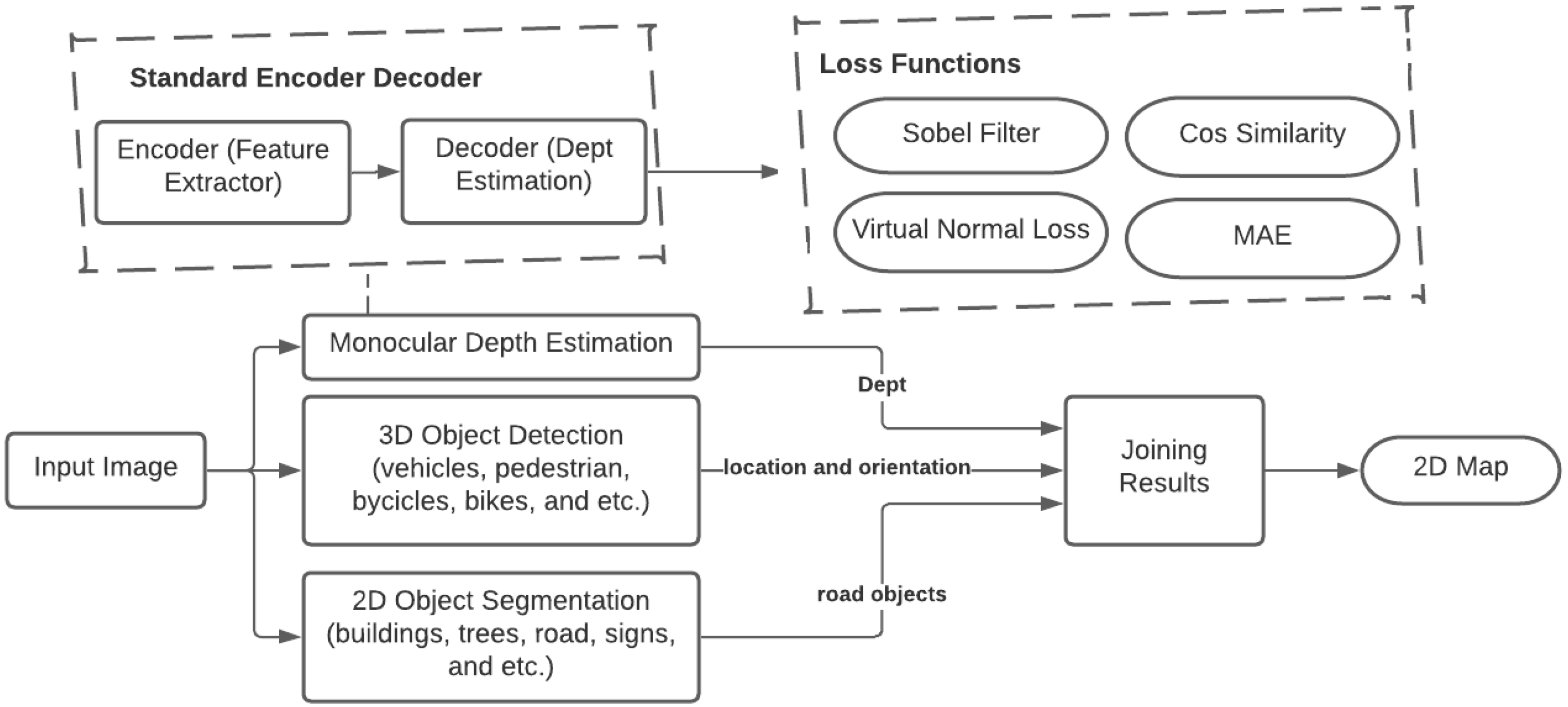
To construct a 2D map from an RGB image, we propose the following main steps (see Figure 1). In the top of the figure, we show the full system architecture to build a 2D map, on the bottom we show our proposed approach for depth estimation: (1) design and train a neural network model for monocular depth estimation to obtain information about the depth of each object in the scene; (2) chose the best 3D object detection model to detect the dynamic objects and their orientation (vehicles, pedestrians, bikes, etc.); and (3) find and enhance a semantic segmentation model to obtain information about the static objects (trees, buildings, etc.).

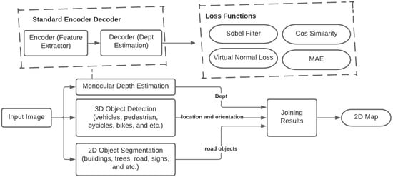
Figure 1. General scheme of the proposed method.

In the scope of this paper, we mostly concentrated on the topic of depth estimation since it is the most important part to reduce running time and memory allocation for 2D map construction. We tried several neural network architectures and the best one is based on the EfficientNetb0 encoder and Nested UNet (UNet++) decoder. We developed the architecture and trained it on our dataset with a hybrid loss function that consists of multiple weighted loss functions (VNL loss, cosine similarity loss, gradient loss, and log MAE loss). We describe in detail the proposed neural network architecture as well as the hybrid loss function in Section 5.

4. Dataset

We used a previously developed platform to collect the data for our dataset in a real environment. To record the data in the vehicle, we used the Drive Safely mobile system (http://mobiledrivesafely.com, accessed on 9 June 2023) developed for Android-based smartphones. The system is a driver assistant and monitoring system which is responsible for detecting dangerous situations in vehicle cabins and providing recommendations to the driver, as well as collecting all information on the cloud server [11]. For the presented paper, the most important information is the data from road cameras.

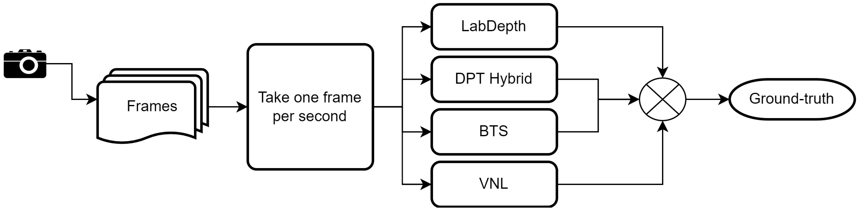
We collected the data from ten drivers that drove vehicles in St. Petersburg, Russia, for a few months. The collected dataset is publicly available at http://doi.org/10.5281/zenodo.8020598 (accessed on 9 June 2023). The image size from the road cameras is 480 × 640. For training, we scaled them down to 420 × 420 and applied center cropping to a 416 × 416 area to exclude border areas that contain noise and distortion. To annotate the data, we used pseudo-labeling and an ensemble of different open-source models that were trained on the KITTI dataset (see Figure 2). The ensemble is based on a weighted mean average using the following weights [0.4, 0.3, 0.2, 0.1] from top to bottom. For each image in the dataset, we used the following four models (LapDept, DTP Hybrid, BTS, and VNL) to obtain the predictions. After that, we took the weighted average between all four masks and saved the results as our ground truth.

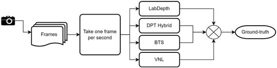
Figure 2. The proposed labeling process for the recorded dataset.

5. Monocular Depth Estimation Model Architecture

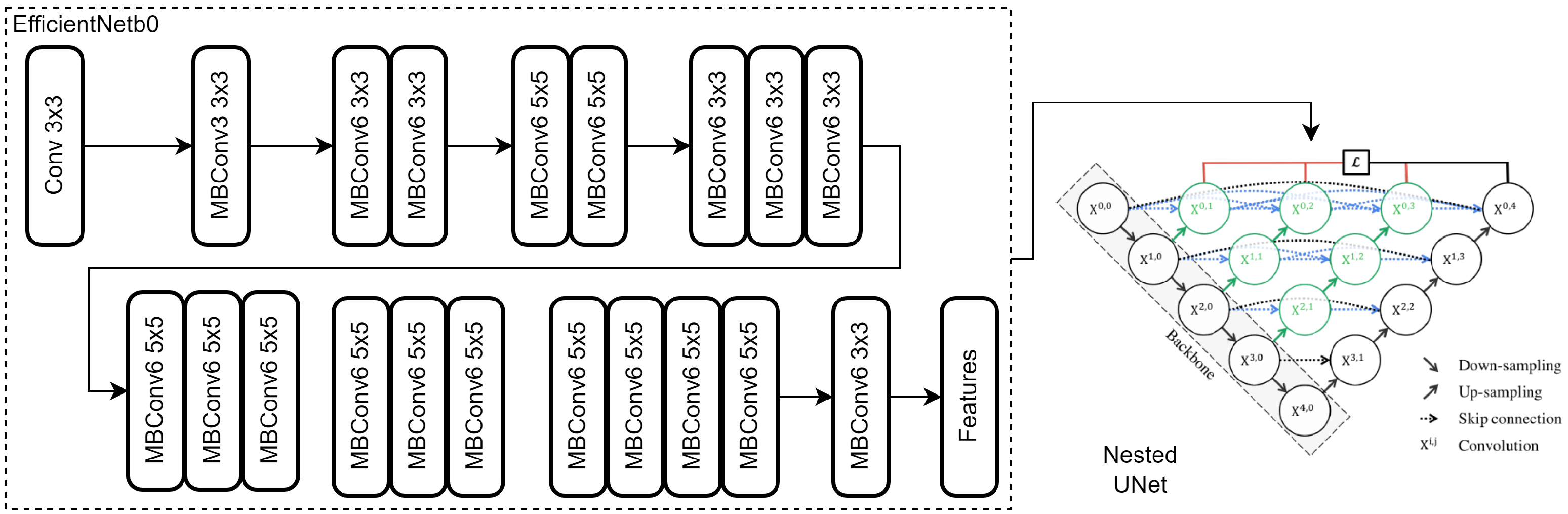
This section describes the proposed efficient depth estimation model with high performance for both evaluation metrics and loss computations, as well as running time, weight size, and parameters (applied to be run on modern smartphones and NVidia Jetson Nano devices). We propose a simple encoder–decoder architecture. The encoder (feature extractor) is MobileNetV3 for smartphones and EfficientNet-b0 [12] for the NVidia Jetson Nano. We chose the UNetPlusPlus architecture as a decoder to minimize the gap between encoder–decoder feature maps and to obtain a better gradient flow. Figure 3 shows the basic architectures of EfficientNet and nested UNet (UNetPlusPlus). We propose a similar architecture for smartphones but replaced EfficientNet-b0 with MobileNetv3. The top part of the figure presents the encoder (feature extractor) that is EfficientNet-b0. For our proposed model, we replaced it with MobileNetv3. The bottom part presents the UNetPlusPlus architecture that consists of similar multiple blocks with decreasing numbers of nodes. The black arrows indicate down-sampling, the red arrows indicate up-sampling, and the dotted arrows indicate skip connections. Each node represents a convolution layer [13].

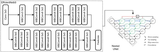
Figure 3. The proposed light-weight efficient depth estimation model [14].

5.1. UNetPlusPlus Architecture

We describe the UNetPlusPlus architecture in detail since it will have a significant effect on depth estimation. The main difference between UNet and nested UNet is that the latter has a loss estimated from four semantic levels (deep supervision named by authors). Nested UNet inherited the dense blocks from the DenseNet architecture as follows.

The output of the previous convolution layers is concatenated with the current convolution by upsampling the lower dense block. The multi-semantic levels will give Nested UNet a more adaptive property to handle the gradient changes in the depth mask that will help to make the architecture itself capable of performing depth estimations without adding more complex layers or heads.

5.2. Loss Functions

The loss function is an important key factor in obtaining a good performance of the neural network model. We suggest a combination of different loss functions to obtain the best performance using a light model: (1) Sobel filter, an image processing technique used for edge extractions by taking the derivatives along the x- and y-axes; (2) mean absolute error (MAE); (3) cos similarity loss, a calculation of the dot product of two vectors (predictions and ground truth); and (4) virtual normal loss (VNL), a method to construct the point cloud from the depth masks and use the camera parameters to project the 2D mask in the 3D space to assure high-order geometric supervision in the 3D space.

To calculate the approximated derivatives for horizontal and vertical changes, we propose a Sobel loss function that can express the changes as follows, where $G_x,G_y$ are the approximated gradients in x, y directions and img is the input image. From the above, we calculate two losses. Multiplying by $\frac{1}{N}$ means taking the average value.

$$G_x=\left[\begin{array}{c}1\\ 2\\ 1\end{array}\right]\ast \left(\left[\begin{array}{ccc}+1& 0& -1\end{array}\right]\ast \mathbf{img}\right)$$

(1)

$$G_y=\left[\begin{array}{c}+1\\ 0\\ -1\end{array}\right]\ast \left(\left[\begin{array}{ccc}1& 2& 1\end{array}\right]\ast \mathbf{img}\right)$$

(2)

$$los{s}_{dx}=log\left(\right|(G_{x_{pred}}-G_{x_{gt}})|+1)\ast \frac{1}{N}$$

(3)

$$los{s}_{dy}=log\left(\right|(G_{y_{pred}}-G_{y_{gt}})|+1)\ast \frac{1}{N}$$

(4)

The log mean absolute error indicates taking the logarithm of the MAE between the predictions and ground truth (gt).

The cosine similarity loss is calculated by the following and we can calculate the loss as the distance.

$$\begin{array}{c}\hfill similarity=\frac{pred.gt}{max\left(\right|\left|pred\right|{|}_2.\left|\right|gt|{|}_2,eps)},los{s}_{cos}=|1-similarity|\ast \frac{1}{N}\end{array}$$

(5)

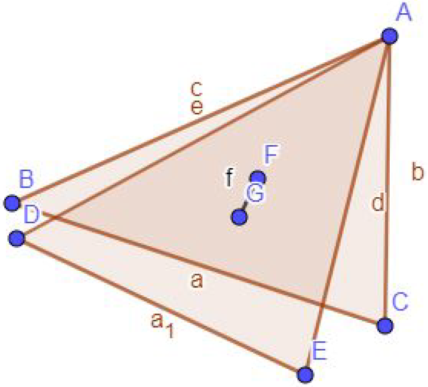
To calculate the virtual normal loss, we chose random multiple groups from the predicted depth mask and their correspondents from the ground truth. Each group consists of three points that are not co-linear (similar to making random triangulations for the depth map). Our goal is to minimize the difference between the centers of these triangles (see Figure 4). Let us assume that triangle ABC is from the predicted depth map and ADE is the corresponding triangle in the ground truth depth mask. F and G are the centers of ABC and ADE, respectively. We minimize the distance f.

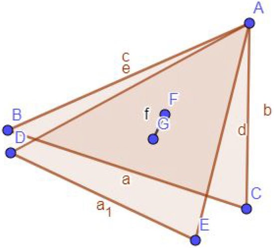
Figure 4. Virtual normal loss clarification.

Thus, we propose $los{s}_{vn}=\frac{1}{M}\ast {\sum }_{i=0}^M{f}_i$, where M is the number of the groups. We propose the hybrid loss to construct the loss function by the following: $loss=a1.los{s}_{vn}+a2.los{s}_{cos}+a3.los{s}_{log-mae}+a4.los{s}_{gradient-loss},$ where a1, a2, a3, and a4 are the coefficients for the weighted average loss. We calculate empirically that for the best results, the following values should be used (0.5, 4, 1, and 1).

Furthermore, we tried to add the chamfer distance to the losses list, which caused worse results by about 2%. This is because of the countering between the chamfer distance and the VN loss. The goal of the former is to minimize the distance between the centers of the triangles and the other is to move the triangles’ corners. On the other hand, the pseudo-labeled ground truth has huge jumps between the depth levels, so it is not suitable to use the chamfer distance. Another idea was to add a discriminator to classify the predictions and the ground truth. The generator (our model) was updated using the proposed loss with the discriminator loss (semi-GAN approach). It did not impact the results, so we decided to remove it.

6. Experiments and Discussion

The main goal of the proposed experiments is to evaluate the proposed model on real data as well as to compare the results obtained with the AdaBins approach, which is the state-of-the-art approach at the moment for monocular depth estimation. We compared both on our recorded dataset as well as on the NYU dataset.

6.1. Running Time

In this subsection, we present the running time for different depth estimation methods as well as for our proposed method (see Table 1). This table shows the running time of different methods for monocular depth estimation on the GPU and CPU. Moreover, it shows the number of parameters for each model (the complexity of the model). The image’s height and width are both equal to 416 in all experiments and the GPU used was a Tesla V100 16 Gb (accessible in Colab Pro). Furthermore, CPU experiments were performed on a Colab CPU. We use Colab for the following reasons: (1) reproducibility (anyone can run tests in the same environment and obtain the same results) and (2) ease of use for most developers.

Table 1. Running time of methods for monocular depth estimation.

Method	Parameters	CPU	GPU
AdaBins	78.257 M	15,000 ms	150 ms
DPT-Hybrid	123.146 M	4200 ms	52 ms
MiDas small	21.320 M	250 ms	17 ms
VNL	115.360 M	5500 ms	73 ms
LapDepth	73.131M	1700 ms	56 ms
Proposed (effb0)	6.569 M	850 ms	15 ms
Proposed (MNv3)	3.007 M	500 ms	10 ms

6.2. Evaluation on the NYU Dataset

We trained our model on over 50 K images from the unlabeled NYU dataset. Unfortunately, due to the difference between the chosen data for training between different methods, it is not a sufficient comparison but it can show an overall perspective of each method (see Table 2). The table shows the evaluation metrics for each method on the NYU dataset. For the RMSE (root mean square error) and ABS_REL (absolute relative error), lower is better, see [15]. log_10 is the log_10 difference between the target and prediction and (Delta1, Delta2, Delta3) presents the accuracy with different thresholds. Ours (large) is the model that uses EfficientNet-b0 as a feature extractor and Ours (small) is the model using MobileNetV3 as a feature extractor.

Table 2. Comparison of the different methods on the NYU dataset.

Method	Encoder	Decoder	RMSE	ABS_REL	log_10	Delta1	Delta2	Delta3
AdaBins	EfficientNet-b5	UNet + miniViT	0.364	0.103	0.044	0.903	0.984	0.997
DPT-Hybrid	ViT transformer	DPT	0.357	0.110	0.045	0.904	0.988	0.998
VNL	ResNext-101 (32 × 4d)	-	0.416	0.111	0.048	0.845	0.976	0.994
LapDepth	ResNext101	Laplacian	0.384	0.105	0.045	0.895	0.983	0.996
Ours (large)	EfficientNet-b0	UNet++	0.514	0.120	0.047	0.825	0.973	0.992

6.3. Evaluation of Recorded Dataset

We trained our model on 7000 images from the pseudo-labeled data for the presented dataset (see Section 4). The goal of this research is to achieve the best performance on the dataset not only in terms of accuracy but also in terms of running time and complexity. The results showed that the proposed model is more than 30 times faster and smaller and it also has a smaller ABS_REl than the state-of-the-art method (see Table 3), where RMSE is the root mean square error, ABS_REL is the absolute relative error (lower is better, see [15]), log_10 is the log_10 difference between target and prediction, and (Delta1, Delta2, Delta3) present the accuracy with different thresholds.

Table 3. Evaluation metrics for each method on our dataset.

Method	Encoder	Decoder	RMSE	ABS_REL	log_10	Delta1	Delta2	Delta3
AdaBins	EfficientNet-b5	UNet + miniViT	0.5136	0.1176	0.0477	0.8638	0.9658	0.9884
Ours (large)	EfficientNet-b0	UNet++	0.5960	0.1173	0.04885	0.8559	0.9597	0.9841
Ours (small)	MobileNetV3	UNet++	0.6088	0.1197	-	0.8494	0.9564	0.9821

6.4. Results

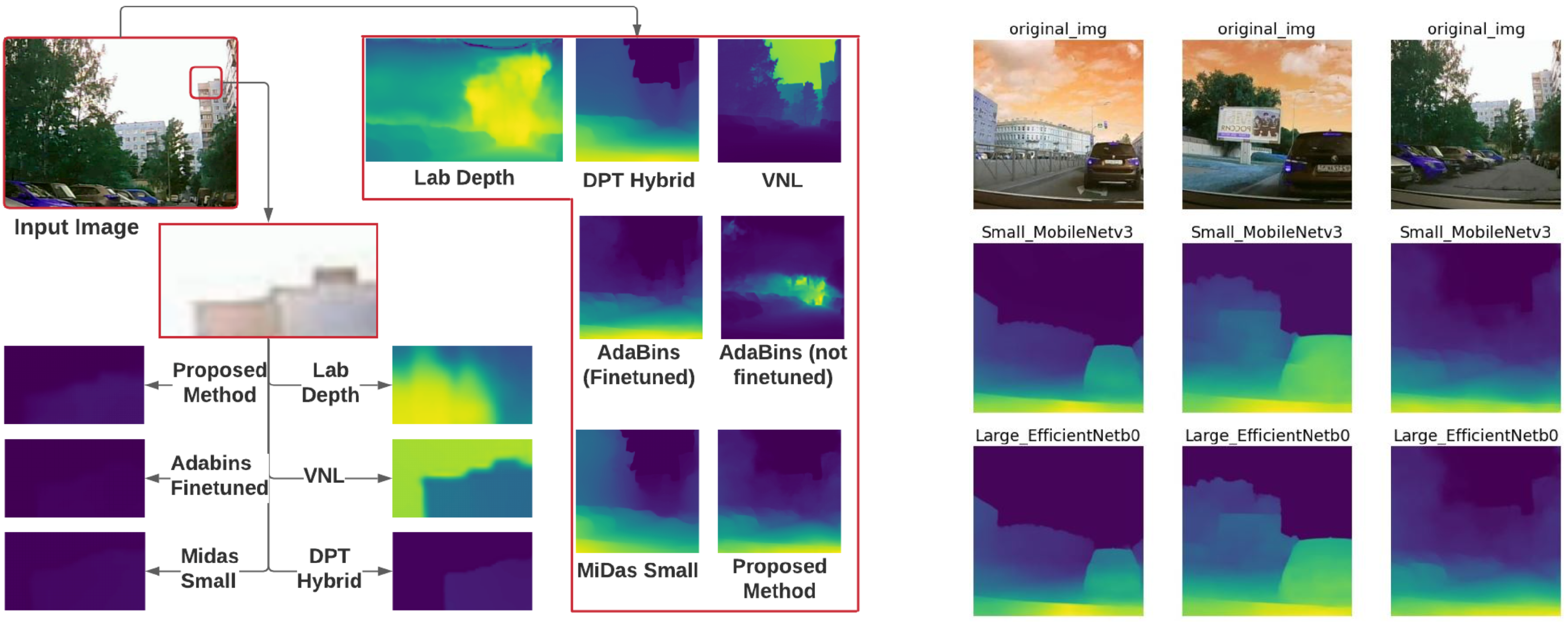
In this section, we present results examples and provide a visual comparison between our small and large models and with the existing methods that were trained on the KITTI dataset as well as on our data. In Figure 5, in the right image we present the depth map output calculated by our method. The first row presents the input images, the second illustrates the output of our small model (MobileNetv3 encoder), and the third is the output of our large model (EfficientNetB0 encoder). The left image presents a visual comparison with other methods.

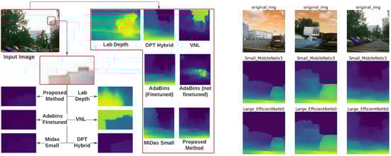
Figure 5. Left image: visual comparison between the methods; right image: depth map output calculated by our method.

7. Conclusions

We introduced a novel approach for real-time depth estimation that includes an efficient neural network architecture and a hybrid loss function. The approach shows competitive results in comparison to the state-of-the-art methods in terms of accuracy, and improvements in terms of running time and size. Based on the presented approach, we propose the method for 2D map construction of vehicle environments. In future work, we will add the Adabins block to our model and investigate its performance on our dataset using the proposed hybrid loss which obtained a less accurate model by 2% in Delta1. We will analyze the method for 3D construction of multiple images and build a model for semantic segmentation and depth estimation.

References

- Subakan, C.; Ravanelli, M.; Cornell, S.; Bronzi, M.; Zhong, J. Attention is all you need in speech separation. In Proceedings of the 2021 IEEE International Conference on Acoustics, Speech and Signal Processing (ICASSP), Toronto, ON, Canada, 6–11 June 2021; pp. 21–25. [Google Scholar]
- Godard, C.; Aodha, O.; Firman, M.; Brostow, G.J. Digging into self-supervised monocular depth estimation. In Proceedings of the IEEE/CVF International Conference on Computer Vision (ICCV), Seoul, Republic of Korea, 27 October–2 November 2019. [Google Scholar]
- Koutilya, P.; Zhou, H.; Jacobs, D. Sharingan: Combining synthetic and real data for unsupervised geometry estimation. In Proceedings of the 2020 IEEE/CVF Conference on Computer Vision and Pattern Recognition (CVPR), Seattle, WA, USA, 13–19 June 2020; pp. 13971–13980. [Google Scholar]
- Johnston, A.; Carneiro, G. Self-supervised monocular trained depth estimation using self-attention and discrete disparity volume. In Proceedings of the 2020 IEEE/CVF Conference on Computer Vision and Pattern Recognition (CVPR), Seattle, WA, USA, 13–19 June 2020; pp. 4755–4764. [Google Scholar]
- Fonder, M.; Ernst, D.; Droogenbroeck, M. M4depth: A motion-based approach for monocular depth estimation on video sequences. arXiv 2021, arXiv:2105.09847. [Google Scholar]
- Ranftl, R.; Lasinger, K.; Hafner, D.; Schindler, K.; Koltun, V. Towards robust monocular depth estimation: Mixing datasets for zero-shot cross-dataset transfer. IEEE Trans. Pattern Anal. Mach. Intell. 2020, 44, 1623–1637. [Google Scholar] [CrossRef] [PubMed]
- Miangoleh, S.M.H.; Dille, S.; Mai, L.; Paris, S.; Aksoy, Y. Boosting monocular depth estimation models to high-resolution via content-adaptive multi-resolution merging. In Proceedings of the 2021 IEEE/CVF Conference on Computer Vision and Pattern Recognition (CVPR), Nashville, TN, USA, 20–25 June 2021; pp. 9680–9689. [Google Scholar]
- Ranftl, R.; Bochkovskiy, A.; Koltun, V. Vision transformers for dense prediction. arXiv 2021, arXiv:2103.13413. [Google Scholar]
- Yin, W.; Liu, Y.; Shen, C.; Yan, Y. Enforcing geometric constraints of virtual normal for depth prediction. In Proceedings of the 2019 IEEE/CVF International Conference on Computer Vision (ICCV), Seoul, Republic of Korea, 27 October–2 November 2019; pp. 5683–5692. [Google Scholar]
- Bhat, S.; Alhashim, I.; Wonka, P. Adabins: Depth estimation using adaptive bins. In Proceedings of the 2021 IEEE/CVF Conference on Computer Vision and Pattern Recognition (CVPR), Nashville, TN, USA, 20–25 June 2021; pp. 4008–4017. [Google Scholar]
- Kashevnik, A.; Lashkov, I.; Ponomarev, A.; Teslya, N.; Gurtov, A. Cloud-Based Driver Monitoring System Using a Smartphone. IEEE Sens. J. 2020, 20, 6701–6715. [Google Scholar] [CrossRef]
- Tan, M.; Le, Q. Efficientnet: Rethinking model scaling for convolutional neural networks. In Proceedings of the 36th International Conference on Machine Learning, Volume 97 of Proceedings of Machine Learning Research, Long Beach, CA, USA, 9–15 June 2019; pp. 6105–6114, PMLR; Electronic Proceedings. [Google Scholar]
- Howard, A.; Sandler, M.; Chen, B.; Wang, W.; Chen, L.; Tan, M.; Chu, G.; Vasudevan, V.; Zhu, Y.; Pang, R.; et al. Searching for mobilenetv3. In Proceedings of the 2019 IEEE/CVF International Conference on Computer Vision (ICCV), Seoul, Republic of Korea, 27 October–2 November 2019; pp. 1314–1324. [Google Scholar]
- Available online: https://sh-tsang.medium.com/review-unet-a-nested-u-net-architecture-biomedical-image-segmentation-57be56859b20 (accessed on 9 June 2023).
- Lyu, X.; Liang, L.; Wang, M.; Kong, X.; Liu, L.; Liu, Y.; Chen, X.; Yuan, Y. Hr-depth: High resolution self-supervised monocular depth estimation. In Proceedings of the AAAI Conference on Artificial Intelligence, Virtually, 2–9 February 2021. [Google Scholar]
Disclaimer/Publisher’s Note: The statements, opinions and data contained in all publications are solely those of the individual author(s) and contributor(s) and not of MDPI and/or the editor(s). MDPI and/or the editor(s) disclaim responsibility for any injury to people or property resulting from any ideas, methods, instructions or products referred to in the content. |
© 2023 by the authors. Licensee MDPI, Basel, Switzerland. This article is an open access article distributed under the terms and conditions of the Creative Commons Attribution (CC BY) license (https://creativecommons.org/licenses/by/4.0/).