Optimization of a Speed Controller of a WECS with Metaheuristic Algorithms ^†

Abstract

This paper describes the modeling and control of a high-power wind energy conversion system (WECS) using a variable speed doubly fed induction generator (DFIG) with the application of an MPPT method to obtain the maximum power from the system. We applied metaheuristic algorithms such as particle swarm optimization algorithms (PSO), Harris hawk optimization (HHO), and salp swarm algorithm (SSA) to optimize the speed sensor. The simulation results indicated that the MPPT method with the proposed optimized sensor could generate optimum rotor speed to achieve maximum power output. The simulation was developed using Matlab/Simulink.

1. Introduction

In recent decades, environmental pollution has been increasing, which is worrying, and conventional energy resources are being consumed rapidly, so the world has been turning to renewable energy resources (RES) [1,2]. RES can cover the entire energy needs of the world. There are many renewable energy resources such as solar, hydroelectric, biomass and wind energy, that have a positive impact [3]. Recently, there has been a serious shortage of power generated by conventional resources, so wind power, with its advantages of low cost and clean energy, is the best choice to meet society’s energy needs. Multiple generators may be used with wind turbines, such as DFIG and permanent magnet synchronous generators (PMSG). DFIG is preferred in this area because it has significant advantages [4]. Variable speed wind turbine (VSWT)-based DFIG is superior to others, in addition to its high performance, due to the light weight, low cost, and small capacity of the converters [2,3,4,5]. To ensure high performance and achieve maximum performance, it is necessary to use an MPPT method [5]. Several types of MPPT methods have been applied to extract maximum power from WECS, such as maximum speed ratio (TSR), and disturbance and observation (D&O). In this study, we are interested in speed servo control, which consists of adjusting the electromagnetic torque of the generator in order to fix the mechanical speed to a reference speed that allows maximum power to be obtained from the turbine, based on the TSR technique extract.

2. Modeling of the WECS

The wind turbine absorbs the kinetic energy of the wind and converts it into torque, which turns the rotor blades. Three factors determine the relationship between the wind energy and the mechanical energy recovered by the rotor: the density of the air, the surface area swept by the rotor, and the wind speed. Air density and wind speed are climatological parameters that depend on site-dependent climatological parameters [6]. The power coefficient Cp characterizes the aerodynamic efficiency of the system (Figure 1). It depends on the characteristics of the turbine (blade dimensions, speed ratio and blade tip angle). We used an empirically approximated expression for a wind turbine using the DFIG-type generator defined as follows [7]:

$$C_p=\left[0.5176\left(\frac{116}{{\lambda }^{\prime }}\right)-0.4\beta -5\right]exp\left(\frac{-21}{{\lambda }^{\prime }}\right)+0.0068\lambda$$

(1)

with:

$${\lambda }^{\prime }=\frac{1}{\lambda +0.08\beta }-\frac{0.035}{{\beta }^3+1}$$

(2)

Figure 1. Power coefficient as a function of the speed ratio (λ) and stall angle (β).

In order to obtain the maximum power from the turbine (Figure 1), $C_p$ and $\lambda$ must have the optimal value for $\lambda =8.1$ and $C_p=0.48$. The mechanical power of the wind turbine and the aerodynamic torque is directly determined by:

$$P_t=0.5C_p\left(\lambda ,\beta \right)\rho \pi R^2{V}^3\mathrm{and}{C}_{aer}=\frac{P_t}{{\mathsf{\Omega }}_t}$$

(3)

The gearbox is the connection between the turbine and the generator. It is used to match the highest speed of the generator to the slowest speed of the turbine. The figure below clarifies the structure of the wind energy conversion system (see Figure 2), and it is often modeled by the following two equations:

$$C_t=\frac{{\mathsf{\Omega }}_{mec}}{G}\mathrm{and} C_g=\frac{{\mathsf{\Omega }}_{aer}}{G}$$

(4)

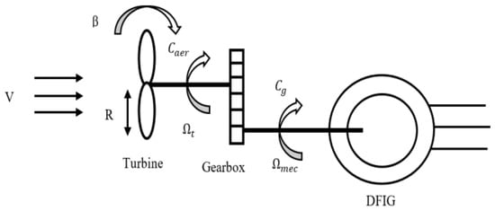
Figure 2. Structure of the wind energy conversion plant.

Modeling of the mechanical transmission can be represented as follows:

$$J\frac{{\mathrm{d}\mathsf{\Omega }}_g}{dt}=C_{mec}=C_g-C_{em}-C_f$$

(5)

The diagram block of the turbine of a horizontal axis variable speed wind turbine is shown in the following figure (Figure 3):

Figure 3. Block diagram of the turbine model.

The MPPT of the Proposed Wind Energy System

The power absorbed by the wind turbine can be maximized by adjusting the coefficient Cp. This coefficient depends on the speed of the generator. It possible to maximize this output using a variable speed wind turbine. It is, therefore, necessary to develop control strategies to maximize the generated electric power (thus, torque) by adjusting the speed of the turbine to its reference value regardless of the wind speed reference value considered as a disturbance variable [8]. The MPPT proposed in this work is the one with known airfoil properties with a control of the speed (the Cp is the one previously defined). This control structure consists of adjusting the torque appearing on the shaft of the Caer turbine in order to fix its speed to a reference value. In order to achieve this, the use of speed control (PI control) is absolutely necessary. The turbine speed reference is that which corresponds to the optimum value of the speed ratio Cpmax (=0, constant), which allows the maximum value of Cp to be obtained. Then we can write:

$${\mathsf{\Omega }}_{ref}=\frac{{\lambda }_{Cpmax}V}{R}$$

(6)

The installation shown in the figure below (Figure 4) represents the implementation of the MPPT with the wind turbine.

Figure 4. Principle of the MPPT proposed for the wind system.

3. DFIG Modeling

The DFIG is a machine that has excelled with its vector control. It is widely used in the wind turbine industry for variable speed wind turbines for various reasons such as the reduction of stress on the mechanical parts, the reduction of noise, and the possibility of controlling active and reactive power. The DFIG model in the d-q reference frame [7] is given by:

$$\{\begin{array}{c}{\mathrm{V}}_{\mathrm{sd}}={\mathrm{R}}_{\mathrm{s}}{\mathrm{i}}_{\mathrm{sd}}+\frac{\mathrm{d}}{\mathrm{dt}}{\mathsf{\phi }}_{\mathrm{sd}}-{\mathrm{w}}_{\mathrm{s}}{\mathsf{\phi }}_{\mathrm{sq}}\\ {\mathrm{V}}_{\mathrm{sq}}={\mathrm{R}}_{\mathrm{s}}{\mathrm{i}}_{\mathrm{sq}}+\frac{\mathrm{d}}{\mathrm{dt}}{\mathsf{\phi }}_{\mathrm{sq}}-{\mathrm{w}}_{\mathrm{s}}{\mathsf{\phi }}_{\mathrm{sd}}\\ {\mathrm{V}}_{\mathrm{rd}}={\mathrm{R}}_{\mathrm{r}}{\mathrm{i}}_{\mathrm{rd}}+\frac{\mathrm{d}}{\mathrm{dt}}{\mathsf{\phi }}_{\mathrm{rd}}-({\mathrm{w}}_{\mathrm{s}}-{\mathrm{w}}_{\mathrm{r}}){\mathsf{\phi }}_{\mathrm{rq}}\\ {\mathrm{V}}_{\mathrm{rq}}={\mathrm{R}}_{\mathrm{r}}{\mathrm{i}}_{\mathrm{rq}}+\frac{\mathrm{d}}{\mathrm{dt}}{\mathsf{\phi }}_{\mathrm{rq}}-({\mathrm{w}}_{\mathrm{s}}-{\mathrm{w}}_{\mathrm{r}}){\mathsf{\phi }}_{\mathrm{rd}}\\ {\mathrm{C}}_{\mathrm{em}}=\frac{3}{2}\mathrm{p}\frac{{\mathrm{L}}_{\mathrm{m}}}{{\mathrm{L}}_{\mathrm{s}}}\left({\mathsf{\phi }}_{\mathrm{qs}}{\mathrm{i}}_{\mathrm{dr}}-{\mathsf{\phi }}_{\mathrm{ds}}{\mathrm{i}}_{\mathrm{qr}}\right)\end{array}$$

(7)

4. Proposed Optimization Algorithm

Metaheuristics are optimization procedures that make it possible to obtain an approximate value of the optimal solution in a reasonable amount of time. The goal is to solve a set of problems in different areas without having to change the basic principle of the algorithm of the method. In our work, we propose three metaheuristic algorithms—particle swarm optimization (PSO), Harris hawks optimization (HHO), and the salp swarm algorithm (SSA)—to see which is best in relation to our system.

4.1. Particle Swarm Optimization (PSO)

PSO is an optimization algorithm based on an evolutionary computational technique. The basic PSO was developed from swarming research such as fish flocking and bird flocking. After first being introduced in 1995, a modified PSO was introduced in 1998 to improve the performance of the original PSO. In PSO, social behavior is modeled by a mathematical equation that allows the particles to be guided during their displacement process [9,10,11,12,13,14,15]. The movement of a particle is influenced by three components: the inertial component, the cognitive component, and the social component. Figure 5 shows a flowchart of the method.

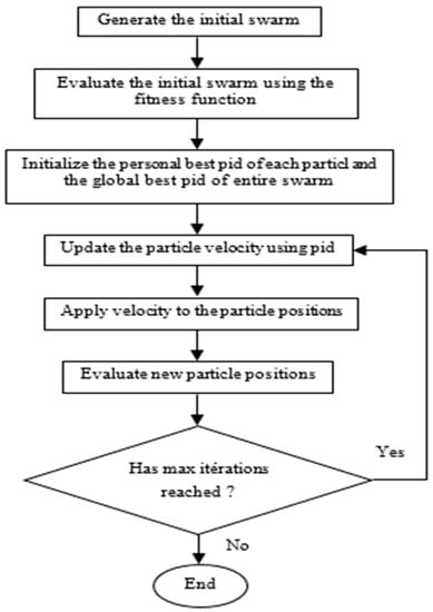
Figure 5. Flowchart of PSO.

4.2. Harris Hawks Optimization (HHO)

The cooperative hunting behavior of Harris hawks has inspired the HHO algorithm and has been mathematically modeled [11,12,13,14]. This algorithm is a population-based algorithm, which was inspired by nature and can be investigated under three main sections of exploration, the transition from exploration to exploitation, along with actual exploitation [14]. The flowchart of the HHO algorithm is shown in Figure 6. The exploration phase of the algorithm mimics the searching behavior of the hawks for prey. This is also the first stage of the algorithm. The mathematical model for this stage has a relation as given in Equation (8) [15]:

$$x\left(\tau +1\right)=\{\begin{array}{c}{x}_r\left(\tau \right)-r_1\left|x_r\left(\tau \right)-2r_{2}x\left(\tau \right)\right|fork\ge 0.5\\ \left(x_p\left(\tau \right)-x_m\left(\tau \right)\right)-r_3\left(L_B+r_4\left(u_B-L_B\right)\right)fork<0.5\end{array}$$

(8)

where $K,r_1,r_2,r_3$ and $r_4$ are random numbers that have a range of [0, 1]. $x_p\left(\tau \right)$ stands for the prey’s position, whereas the current and the next positions of the hawk are shown by $x\left(\tau \right)$ and $x\left(\tau +1\right)$, respectively. The random numbers of $r_1,r_2, r_3$ and $r_4$ are updated in each iteration. $U_B$ and $L_B$ are the search space’s upper and lower bounds, respectively. $x_r\left(\tau \right)$ and x_m represent a randomly selected hawk in the available population and the average position of the population of hawks, respectively.

Figure 6. Flowchart of HHO.

4.3. Salp Swarm Algorithm (SSA)

SSA is one of the random population-based algorithms suggested by Mirjalili [12]. SSA simulates the swarming mechanism of salps when foraging in oceans. In heavy oceans, salps usually shape a swarm known as a salp chain. In the SSA algorithm, the leader is the salp at the front of the chain, and the remainder of salps are called followers. As with other swarm-based techniques, the position of the salps is defined in an s-dimensional search space, where s is the number of variables in a given problem. Therefore, the position of all salps is stored in a two-dimensional matrix called z. It is also assumed that there is a food source called P in the search space as the swarm’s target. The mathematical model for SSA is given as follows: The leader salp can change position by using the next equation [12,13,14]:

$$z_n^1=\{\begin{array}{c}{P}_n+r_1\left((U_n-l_n\right)r_2+l_n) r_3\ge 0\\ P_n-r_1\left((U_n-l_n\right)r_2+l_n) r_3<0\end{array}$$

(9)

where the meanings of all symbols are shown in Table 1.

$$r_1=2e^{-}{\left(-\frac{4a}{A}\right)}^2$$

(10)

Table 1. The meanings of all symbols.

Symbols	Meaning
$z_n^1$	leader position in nth dimension
$P_n$	food source position in nth dimension
$U_n$	upper bound of nth dimension
$l_n$	lower bound of nth dimension
r1, r2, and r3	random variables uniformly produced in the interval of [0, 1]
a	current iteration
A	maximum number of iterations
$z_n^m$	position of mith follower salp in nth dimension
e	time
$v_0$	initial speed

The coefficient r₁ is the essential parameter in SSA because it provides a balance between exploration and exploitation capabilities. To change the position of the followers, the next equations are utilized [16]:

$$z_n^m=\frac{1}{2}c{e}^2+v_{0}e$$

(11)

The flowchart of this algorithm is given as follows in Figure 7:

Figure 7. Flowchart of SSA.

5. Results and Discussion

In the simulation, the analysis was carried out in Matlab/Simulink. We present the results obtained for the dual-feed asynchronous generator (DFIG) with the application of the metaheuristic algorithm to optimize the parameters of the speed controller that provides the maximum power of the wind turbine; Figure 7 represents the block diagram used for the controller with the implementation of the applied optimization algorithms (Figure 8), which is widely used in the literature to evaluate the performance of PID controller design [13,14,15]. Rather than evaluating these error criteria as the objective alone, Zwe-Lee Gaing’s study showed that objective combinations of these error criteria, which include eight factors, are a better way to form a common goal [15,16]. Many researchers use the method presented there. Four indices are commonly used to represent system performance: square integral error (ISE), absolute integral error (IAE), absolute temporal integral error (ITAE), and square temporal integral error (ITSE). They are defined as follows:

$$\begin{array}{c}IAE={{\displaystyle \int }}^{\text{}}\left|e\left(t\right)\right|dt\\ ITAE={{\displaystyle \int }}^{\text{}}t.\left|e\left(t\right)\right|dt\\ ISE={{\displaystyle \int }}^{\text{}}e{\left(t\right)}^{2}dt\\ ITSE={{\displaystyle \int }}^{\text{}}t.\left|e{\left(t\right)}^2\right|dt\end{array}$$

(12)

Figure 8. The block diagram of the implementation of the optimization algorithm for the speed turbine control.

The table below (Table 2) presents the different parameters obtained through the optimization, showing the best results for each algorithm after several tests.

Table 2. The different results obtained by optimization.

Algorithm	ISE	ITSE	IAE	ITAE	Error
PSO-Kp	19.3738	1.5885	23.2340	0.0001	0.4733
PSO-Ki	0.0001	28.5724	0.0001	17.9310
HHO-Kp	50	50	37.0073	50	0.0023
HHO-Ki	34.9314	50	33.8005	30.0855
SSA-Kp	50	50	50	34.2211	0.0003
SSA-Ki	29.9746	34.9321	3.1388	31.7244

The colored values in the table are the best for minimum error for each algorithm used. The following figures show the evolution of various system parameters as a function of time for an average wind speed of 12 m/s and zero setting angle.

Table 2 presents the figures obtained by the most powerful algorithm, the SSA. We note that the SSA algorithm provided the optimal power coefficient Cp = 0.49 with a stall angle $\beta$ = 0 (Figure 9) and a speed ratio $\lambda$ = 8.1 as shown in Figure 10. Figure 11 shows the speed curve plotted with the reference speed, showing a minimum error of ${3 \times 10}^{-3}$ and a stabilization time of $1.0274 \times {10}^5$ s, where Figure 12 and Figure 13 represent, respectively, the active and reactive power stabilizing at 100 s.

Figure 9. Power coefficient (with SSA).

Figure 10. Speed ratio (with SSA).

Figure 11. Mechanical speed (with SSA).

Figure 12. Variation of the stator active power (with SSA).

Figure 13. Variation of the stator reactive power (with SSA).

6. Conclusions

We proposed a full modeling of the VS-WECS in this paper. The system was based on a 1.5 MW DFIG, and the modeling and simulation of the wind turbine conversion chain were performed with a control architecture (MPPT) that maximized energy efficiency. Therefore, we played, on the one hand, on the efficiency of the conversion chain, and on the other hand, on the quality of the reactive power. To extract maximum power, we used a PI speed controller optimized with metaheuristic algorithms (PSO, HHO and SSA). The results obtained with the salp swarm approach (SSA) confirmed the effectiveness of our approach (stability and minimization of the wind turbine speed error). In future work, we will investigate the application of our approach to optimize a grid-connected wind farm.

References

- Sun, H.; Han, Y.; Zhang, L. Maximum Wind Power Tracking of Doubly Fed Wind Turbine System Based on Adaptive Gain Second-Order Sliding Mode. J. Control Sci. Eng. 2018, 2018, 1–11. [Google Scholar] [CrossRef]
- Abdou, E.H.; Abdel-Raheem, Y.; Kamel, S.; Aly, M.M. Sensorless Wind Speed Control of 1.5 MW DFIG Wind Turbines for MPPT. In Proceedings of the Twentieth International Middle East Power Systems Conference (MEPCON), Cairo, Egypt, 18–20 December 2018; Cairo University: Giza, Egypt, 2018; pp. 700–704. [Google Scholar]
- Kaloi, G.S.; Wang, J.; Baloch, M.H. Active and reactive power control of the doubly fed induction generator based on wind energy conversion system. Energy Rep. 2016, 2, 194–200. [Google Scholar] [CrossRef]
- Yin, M.; Xu, Y.; Shen, C.; Liu, J.; Dong, Z.Y.; Zou, Y. Turbine Stability-Constrained Available Wind Power of Variable Speed Wind Turbines for Active Power Control. IEEE Trans. Power Syst. 2017, 32, 2487–2488. [Google Scholar] [CrossRef]
- Falehi, A.D.; Rafiee, M. Maximum efficiency of wind energy using novel Dynamic Voltage Restorer for DFIG based Wind Turbine. Energy Rep. 2018, 4, 308–322. [Google Scholar] [CrossRef]
- Mirecki, A. Etude Comparative de Chaînes de Conversion d’Energie Dédiées à une Eolienne de Petite Puissance. Ph.D. Thesis, Institut National Polytechnique de Toulouse, Toulouse, France, 2005; p. 252. [Google Scholar]
- Djarir, Y. Commande Directe du Couple et des Puissances d’une MADA Associée à un Système Eolien par les Techniques de L’intelligence Artificielle. Ph.D. Thesis, Université Djilali LIABES Sidi-Bel-Abbès, Sidi Bel Abbès, Algeria, 2015; p. 285. [Google Scholar]
- Modeling, Identification and Control Methods in Renewable Energy Systems; Springer Science and Business Media LLC: Marrakech, Morocco, 2019; pp. 1–374.
- Sulaiman, D.R. Multi-objective Pareto front and particle swarm optimization algorithms for power dissipation reduction in microprocessors. Int. J. Electr. Comput. Eng. (IJECE) 2020, 10, 6549–6557. [Google Scholar] [CrossRef]
- Rani, V.L.; Latha, M.M. Particle Swarm Optimization Algorithm for Leakage Power Reduction in VLSI Circuits. Int. J. Electron. Telecommun. 2016, 62, 179–186. [Google Scholar] [CrossRef]
- Izci, D.; Ekinci, S.; Demiroren, A.; Hedley, J. HHO Algorithm based PID Controller Design for Aircraft Pitch Angle Control System. In Proceedings of the International Congress on Human-Computer Interaction, Optimization and Robotic Applications (HORA), Ankara, Turkey, 26–28 June 2020; p. 6. [Google Scholar]
- Hegazy, A.E.; Makhlouf, M.A.; El-Tawel, G.S. Improved Salp Swarm Algorithm for Feature Selection. J. King Saud Univ. Comput. Inf. Sci. 2020, 32, 335–344. [Google Scholar] [CrossRef]
- Kennedy, J.; Eberhart, R. Particle Swarm Optimization. In Proceedings of the IEEE International Joint Conference on Neural Networks, Perth, WA, Australia, 27 November–1 December 1995; pp. 1943–1948. [Google Scholar]
- Heidari, A.A.; Mirjalili, S.; Faris, H.; Aljarah, I.; Mafarja, M.; Chen, H. Harris hawks optimization: Algorithm and applications. Futur. Gener. Comput. Syst. 2019, 97, 849–872. [Google Scholar] [CrossRef]
- Gaing, Z.-L. A Particle Swarm Optimization Approach for Optimum Design of PID Controller in AVR System. IEEE Trans. Energy Convers. 2004, 19, 384–391. [Google Scholar] [CrossRef]
- Kose, E. Optimal Control of AVR System with Tree Seed Algorithm-Based PID Controller. IEEE Access 2020, 8, 89457–89467. [Google Scholar] [CrossRef]
Disclaimer/Publisher’s Note: The statements, opinions and data contained in all publications are solely those of the individual author(s) and contributor(s) and not of MDPI and/or the editor(s). MDPI and/or the editor(s) disclaim responsibility for any injury to people or property resulting from any ideas, methods, instructions or products referred to in the content. |
© 2023 by the authors. Licensee MDPI, Basel, Switzerland. This article is an open access article distributed under the terms and conditions of the Creative Commons Attribution (CC BY) license (https://creativecommons.org/licenses/by/4.0/).