Pathloss Estimation of Digital Terrestrial Television Communication Link Within the UHF Band

Abstract

The global shift to digital terrestrial television broadcasting (DTTB) from the conventional analogue has significantly transformed television culture, necessitating comprehensive technical and infrastructural evaluations. This study addresses the limitations of existing path-loss models for accurately predicting path loss in digital terrestrial television broadcasting in the UHF bands, motivated by the need for reliable, location-specific models that account for seasonal, meteorological, and topographical variations in Abeokuta, Nigeria. The study focuses on path-loss prediction in the UHF band using Ogun State Television (OGTV), Abeokuta, Nigeria, as the transmission source. Eight receiving sites, spaced 2 kilometers apart, were selected along a 16.7 km transmission contour. Daily measurements of received signal strength (RSS) and weather conditions were collected over one year. Seasonal path-loss models ${PL}_{wet}$ for the wet season and ${PL}_{dry}$. For the dry season, models were developed using multiple regression analysis and further optimized using least squares (LS) and gradient descent (GD) techniques, resulting in six refined models: ${PL}_{wet}$, ${PL}_{dry}$, ${PL}_{wet-LS}$, ${PL}_{dry-LS}$, ${PL}_{wet-GD}$, and ${PL}_{dry-GD}$. Model performance was evaluated using Mean Absolute Error, Root Mean Square Error, Coefficient of Correlation, and Coefficient of Multiple Determination. Results indicate that the Okumura model provided the closest approximation to measured RSS for all the receiving sites, while the Hata and COST-231 models were unsuitable. Among the developed models, ${PL}_{wet}$ ($RMSE- 1.2633$, $MAE - 0.9968$, $MSE - 1.5959$, $R - 0.9935$, $R^2 - 0.9871$) and ${PL}_{dry-LS}$($RMSE- 1.1884$, $MAE - 0.7692$, $MSE - 1.4124$, $R - 0.9942$, $R^2 - 0.9883$) were found to be the most suitable models for the wet and dry seasons, respectively. The major influence of location-based elevation and meteorological data on path-loss prediction over digital terrestrial television broadcasting communication lines in Ultra-High-Frequency bands was evident.

1. Introduction

Wireless communication fundamentally depends on the propagation of electromagnetic (EM) waves from a transmitting source to a receiving point. As these waves travel through various media, the received signal experiences path loss, a gradual reduction in power shaped by environmental and atmospheric conditions. Igwe et al. [1] note that this attenuation arises from mechanisms such as reflection, diffraction, and scattering, which occur when EM waves interact with terrain features, vegetation, obstacles, and irregular atmospheric layers. In the UHF band, where wavelengths are short and comparable in size to buildings, vehicles, and trees, these interactions are especially significant. As a result, UHF signals often experience multipath fading, terrain obstruction, and attenuation due to atmospheric moisture—factors that collectively reduce signal reliability, particularly in urban and suburban environments [2].

These challenges make accurate prediction of received signal strength (RSS) both technically necessary and practically difficult. Rapaport [3] emphasizes that the complexity of real propagation environments complicates signal prediction, necessitating the use of path-loss models that account for local conditions. As wireless systems continue to grow in scale and performance requirements, accurate estimation of base station locations, coverage areas, and interference levels has become essential to achieve reliable quality of service (QoS) [4]. However, environmental variables such as terrain elevation, building density, foliage, temperature, humidity, and pressure cause spatial and temporal variations in signal behavior that generic models often fail to capture [5].

In Digital Terrestrial Television (DTTV) systems, these propagation issues are especially critical. DTTV represents a significant advancement over analogue broadcasting, allowing efficient digital encoding, improved picture and sound quality, and enhanced data services [6,7]. Its performance, however, depends heavily on the accuracy of UHF path-loss prediction because signal degradation directly affects coverage uniformity and viewing quality. The sensitivity of UHF signals to changing meteorological conditions further underscores the need for reliable, locally adapted propagation models, especially in regions with diverse weather patterns throughout the year [8,9].

Although numerous empirical and deterministic path-loss models have been proposed and applied globally, their performance varies significantly across different environments. Many existing studies highlight the limitations of applying generalized models to highly variable or complex terrains without calibration. Recent advances in supervised machine learning offer an opportunity to address these limitations, as ML models have demonstrated superior accuracy and computational efficiency by learning directly from measured field data [10,11]. These capabilities allow them to capture nonlinear propagation patterns that traditional models often oversimplify.

Motivated by these considerations, this study focuses on developing an accurate and locally optimized path-loss prediction model for DTTV communication links within selected sites in Abeokuta. The study involves extensive field measurements of received signal strength under varying weather conditions to capture the actual propagation behavior of UHF signals in the study area. Using these measurements as a baseline, a new empirical model is formulated and subsequently optimized using gradient descent and least-squares algorithms to enhance its predictive capability and stability. The final model is rigorously evaluated using five widely accepted statistical performance metrics and benchmarked against standard empirical models to determine its suitability for DTTV planning and deployment in the region.

1.1. Contribution

This study makes several significant contributions to improving path-loss prediction for Digital Terrestrial Television Broadcasting (DTTB) in the UHF band. The study introduces season-specific path-loss models, ${PL}_{wet}$ and ${PL}_{dry}$ developed through multiple regression analysis of empirical data collected over a whole year, allowing for more accurate signal prediction under varying tropical weather conditions. These models were further optimized using gradient descent and least squares techniques to produce four enhanced variants, significantly improving predictive accuracy. A comprehensive empirical dataset was compiled from eight receiver locations along a 16.7 km contour in Abeokuta, Nigeria, with daily measurements of received signal strength and weather parameters, enriching the models with both spatial and temporal depth.

The study conducted a comprehensive comparative analysis of classical path-loss models, including the Okumura, Hata, and COST-231 models, to evaluate their performance under local environmental conditions. Among these, the Okumura model was identified as the most accurate and reliable for predicting path loss in the study area, while the limitations of the other models were also clearly highlighted. Additionally, the research introduced and validated two context-specific models, PL_wet and PL_dry−LS, which proved to be the most effective for the wet and dry seasons, respectively. This demonstrates the importance of adopting context-aware modeling for improved prediction accuracy.

Furthermore, the study revealed that elevation and key meteorological variables, such as humidity and rainfall, exert a substantial influence on UHF signal propagation, underscoring the need for localized, data-driven approaches in terrestrial broadcast network planning. Collectively, these findings provide valuable insights and practical tools to enhance the design, optimization, and reliability of Digital Terrestrial Television Broadcasting (DTTB) networks, particularly in regions with diverse topographical features and varying climatic conditions.

1.2. Paper Organization

The remaining parts of this paper are organized as follows: Section 2 examines existing research and models for path-loss prediction across various environments. It highlights the strengths and limitations of empirical, deterministic, and machine-learning-based models, and discusses gaps in current knowledge. The review also emphasizes the need for localized models that account for environmental factors such as weather, terrain, and urban density, particularly in Sub-Saharan African contexts. A summary table compares key studies, their methodologies, and their relevance to the present work.

Section 3 describes the study area (Abeokuta, Nigeria) and outlines the data collection process, including the tools and equipment used (e.g., GPS units, signal-strength meters, weather stations). It explains how signal strength and meteorological data were collected at eight different sites over the course of a year. It also details the development of seasonal path-loss models using multiple regression analysis, and their subsequent optimization using Least Squares (LS) and Gradient Descent (GD) techniques.

At the same time, Section 4 presents the empirical findings, including measured signal strength, actual path-loss values during wet and dry seasons, and predicted values from the developed models. It compares the proposed models to empirical models (Hata, Okumura, ECC-33), showing that the proposed models, especially ${PL}_{wet}$ and ${PL}_{dry-LS},$ offer better prediction accuracy. The discussion includes statistical evaluations using metrics like $RMSE, MAE, \mathrm{a}\mathrm{n}\mathrm{d} R^2$. It also demonstrates the influence of elevation and weather conditions on signal attenuation and validates the superiority of the proposed models through visual graphs and performance tables.

The conclusion in Section 5 summarizes the research contributions, including the development of season-specific path-loss models and the successful application of optimization techniques. It highlights the models’ improved accuracy over classical alternatives and their practical utility for network planning in tropical regions. The section also acknowledges limitations, such as the geographic scope and the lack of multi-band analysis, and recommends future work to generalize and extend the findings.

2. Related Work

Radio signals, when received at a distance from the transmitter, can manifest in various forms, thereby demonstrating the intricate nature of signal propagation. These forms encompass direct transmissions, in which the signal travels a straightforward path from the transmitter to the receiver. Additionally, reflected waves represent another manifestation, as the signal ricochets off various surfaces or atmospheric layers before ultimately reaching the receiver. Several factors contribute to the phenomenon of signal reception via multiple paths. Terrain, such as hills or valleys, can obstruct the signal’s direct path, leading to reflections or diffractions.

The composition of the atmosphere and the presence of various terrestrial objects also influence how radio signals propagate. As a result, understanding these factors and their impacts is crucial for designing and operating effective terrestrial television broadcasting systems, as they can affect signal quality, coverage, and reliability. Researchers such as Okoro and Agbo [12] and Akinbolati et al. [13] have explored these complexities, shedding light on the intricacies of signal propagation under various conditions and environments.

Various environmental factors can influence the behavior of UHF signals, adding another layer of complexity to their propagation. Precipitation, for instance, can weaken UHF signals, a phenomenon investigated in [14]. Rain and other forms of precipitation can scatter or absorb UHF signals, resulting in signal loss and reduced coverage. Understanding these effects is crucial to maintaining reliable TV broadcasts in areas with changing weather. Additionally, changes in atmospheric refractive index within the troposphere significantly influence radio wave propagation. This effect is not merely an obscure occurrence but a well-established and extensively investigated phenomenon, as evidenced by [15]. These fluctuations in refractive index can cause deviations in the path of radio waves, ultimately leading to signal attenuation.

Accurate models and predictions of radio signal behavior in various atmospheric conditions are vital for ensuring the reliability and performance of terrestrial television broadcasting systems. As noted by [16], understanding radio refractivity is pivotal for addressing the technical and operational aspects of radio communication, ensuring that signals reach their intended destinations with minimal interference and attenuation.

Adopting path loss models for radio network planning and optimization offers several benefits. One of these is cost savings by minimizing extensive trial-and-error deployments. It also saves time by providing a reliable framework for network design and configuration. This efficiency is critical in rapidly evolving and expanding wireless communication networks [10,11]. Notable empirical macrocellular environment models include the Hata, Okumura, and COST-231 Hata models, which have been instrumental in the field of wireless communication. These models have evolved to predict path loss across various scenarios and frequency ranges accurately. It is worth noting that this model needs to be expanded and refined for higher frequencies to ensure its applicability in modern wireless communication systems. These models consider various parameters when estimating mean path loss. These parameters include the heights of the transmitter and receiver antennas, as well as the separation between them [17,18].

As technology and communication networks continue to evolve rapidly, the application of empirical macrocellular environment models will remain essential to advancing the efficiency and reliability of wireless communication systems. These models provide critical insights into how signals propagate across complex environments, enabling engineers to predict coverage, minimize interference, and optimize overall network performance. By facilitating more accurate planning and design of communication infrastructures, they help ensure consistent signal reliability, improved quality of service, and effective resource utilization. Ultimately, as user demands and data traffic continue to increase, these models will serve as indispensable tools in meeting the growing and dynamic requirements of modern wireless communication networks.

Zhang et al. [19] presented an innovative methodology for modeling Air-to-Air (AA) path loss by leveraging machine learning techniques to enhance prediction accuracy in complex urban environments. In their study, ray-tracing software was utilized to generate both training and testing datasets, specifically tailored to represent an urban AA communication scenario. To construct the path-loss prediction framework, the researchers employed two prominent machine learning algorithms—Random Forest (RF) and K-Nearest Neighbors (KNN). They compared their predictive performance against two well-established empirical models. This comparative analysis aimed to assess the accuracy of machine-learning-based models in estimating path loss along AA communication routes in urban settings. The findings revealed that the machine learning models, notably the Random Forest algorithm, demonstrated superior flexibility and predictive accuracy, effectively capturing the complex interactions of signal propagation in urban environments. These results reveal the potential of data-driven approaches as powerful alternatives to traditional empirical models for path-loss prediction in next-generation aerial communication systems.

The performance of these models depended on the quality of the training data used. Additionally, the research emphasized the importance of various input parameters in modeling AA path loss. Path visibility was identified as the most critical factor influencing path loss among the parameters studied, followed by propagation distance and elevation angle. These findings are on the deployment of air-to-air communication systems in urban environments.

The study by Garcia et al. [20] aimed to improve the predictive accuracy of the ITU-R model for estimating path loss in Digital Terrestrial Television channels. By employing the ITU-R P.1812-4 model as the foundational framework, the researchers integrated field-measured data to better capture real-world propagation characteristics. Subsequently, they applied the Particle Swarm Optimization (PSO) algorithm to fine-tune the model parameters. This improvement in accuracy was demonstrated through metrics such as Root Mean Square Error (RMSE), Grey Relation Grade, and Mean Absolute Percentage Error (GRC-MAPE). The research findings suggested that the PSO technique has broader applications and can be employed in various telecommunication systems or measurement environments. This highlights the versatility and potential utility of the PSO approach for enhancing path-loss predictions across different contexts.

Bakare and Ekeocha [21] discussed the technical features of DTTV transmission, its development, potentials, and obstacles in Nigeria. Their findings suggest that DTTV has a promising future if the issues with electricity and government regulations are resolved. Additionally, they argued that maintaining the digitization process depends on effective policy management and government cooperation. Bendov [22] investigated the Notice of Proposed Rulemaking (NPRM) addressing potential interference from unlicensed devices transmitting on frequencies associated with vacated DTTV channels. He discovered how detrimental adjacent and co-channel interferences are to DTV channels. Additionally, he noted that grouping DTV channels in each primary market into a block of adjacent channels would free significant amounts of valuable spectrum while protecting DTV stations from harmful interference.

Akinbolati and Ajewole [16] conducted a comprehensive study of path-loss variation with distance in Digital Terrestrial Television (DTT) systems, focusing on the performance of the Okumura-Hata and Modified Okumura-Hata Path Loss (MOHPL) models. Their findings revealed a consistent and progressive increase in the path loss predicted by the Okumura-Hata model as the Line-of-Sight (LOS) separation distance from the Digital Terrestrial Television Base Station (DTTBS) increased. This pattern remained steady across different routes and seasonal conditions, exhibiting a characteristic exponential growth trend.

Conversely, the MOHPL model displayed a similar increasing trend, but with intermittent fluctuations—marked by peaks and valleys—suggesting the influence of varying environmental and meteorological factors, such as terrain elevation, building density, humidity, and temperature gradients, which collectively affect signal propagation. These results highlight the limitations of conventional empirical models when applied to diverse and dynamic environments, underscoring the need for local calibration or hybrid modeling to achieve greater predictive accuracy. The study therefore recommends the use of high-power transmitters or the installation of repeater stations to strengthen signal coverage and maintain optimal service quality over longer distances. Such measures are crucial for mitigating the adverse effects of path loss associated with extended LOS separations, thereby ensuring consistent and reliable DTT signal reception across regions with complex topographical and climatic conditions.

In their study, Ojo et al. [23] presented a robust, innovative three-phase methodology to overcome the limitations of traditional empirical and deterministic path-loss models. The research began with an extensive drive test conducted across six base transceiver stations (BTS) in Cyprus, specifically targeting multi-transmitter environments, which present more intricate propagation challenges due to signal interference and overlapping coverage areas compared to single-transmitter setups. Using data from these real-world measurements, the authors developed two machine learning-based path-loss models: the Radial Basis Function Neural Network (RBFNN) and the Multilayer Perceptron Neural Network (MLPNN). These models were designed to leverage data-driven learning to capture the nonlinear relationships between environmental variables and path loss characteristics, which conventional models often fail to represent accurately.

In the final phase, both models were evaluated against measured path loss data using key statistical performance metrics, such as the Root Mean Squared Error (RMSE), to assess their predictive accuracy. The findings demonstrated that the RBFNN model achieved superior accuracy and generalization performance compared to the MLPNN, confirming its effectiveness in modeling complex multi-transmitter signal propagation scenarios. This work highlights the potential of machine learning algorithms to enhance path-loss modeling, particularly in modern LTE and next-generation wireless communication systems, where environmental diversity and signal interactions are crucial factors in network planning and optimization.

Moraitis et al. [24] conducted an extensive investigation to improve path-loss prediction accuracy in rural regions of Greece, where complex terrain and sparse network infrastructure often distort radio-wave propagation. To achieve this, the researchers applied several machine learning techniques, including Artificial Neural Networks (ANN), Support Vector Regression (SVR), Random Forest (RF), and Bagging with k-Nearest Neighbors (B-kNN). These algorithms were trained and tested using point-to-multipoint signal measurements collected at 3.7 GHz from multiple rural sites, representing diverse propagation conditions. The goal of the study was to determine which model would provide the most reliable and precise path loss predictions.

The experimental results showed that the machine learning models performed considerably better than traditional empirical path-loss models, with Root Mean Square Error (RMSE) values ranging from 4.0 to 6.5 dB, indicating greater accuracy in modeling signal attenuation. Among the evaluated techniques, the SVR model with a polynomial kernel showed the lowest prediction accuracy. At the same time, RF and B-kNN methods produced very close, more stable results, with low RMSE values of approximately 4.2–4.3 dB. Additionally, the study investigated how varying the ANN structure affected performance. It was found that increasing the number of hidden layers enhanced prediction capability up to three layers, beyond which improvements became minimal.

The optimal configuration—a three-hidden-layer ANN with 51 neurons distributed evenly across the layers—achieved the best results, with an RMSE of 4.0 dB. Overall, the findings highlight that adopting machine learning-driven models, particularly ANN, RF, and B-kNN, can significantly improve the accuracy of path loss prediction in rural wireless communication networks, enabling more efficient planning and enhanced signal reliability in topographically diverse areas.

In a recent investigation [25], researchers proposed an advanced Artificial Neural Network (ANN)-based path-loss prediction model to enhance the accuracy and adaptability of radio propagation forecasting across diverse environments. The model was developed using an extensive dataset comprising path-loss measurements from 485 base stations distributed across six major cities in Nigeria, collected over 9 years. This comprehensive dataset captured variations across different terrain types, including open rural landscapes, suburban regions, and densely built urban zones. It spanned a broad frequency range from 89.3 MHz to 2100 MHz, providing a rich and diverse training foundation for the model. When evaluated, the ANN-based model demonstrated superior predictive accuracy compared to conventional empirical and deterministic models, particularly in handling multi-frequency data and adapting to varying propagation conditions. Its average Root Mean Square Error (RMSE) values consistently fell within acceptable engineering limits, emphasizing its reliability and precision.

Notably, the model’s multi-frequency adaptability enables it to function effectively across both short-range and long-range communication networks, making it highly suitable for deployment in heterogeneous environments where signal behavior varies with topography and frequency. This research presents a significant advancement in data-driven wireless propagation modeling, illustrating how ANN techniques can bridge the gap between empirical estimation and real-world propagation dynamics in the rapidly evolving field of wireless communications.

In a recent performance analysis conducted by Ukatu and Meneya [26], path loss models for digital terrestrial transmission were examined in both urban and rural environments, with a focus on GoTV antennas in Nigeria. The objective was to compare the performance of various empirical models in these diverse settings. The study’s findings revealed that the Hata model was well-suited for predicting path loss in urban environments. This model demonstrated strong predictive capabilities and reliable capture of the complex propagation characteristics of urban settings, making it a valuable choice for digital terrestrial transmission modeling in these areas.

Conversely, the CCIR model was identified as a suitable choice for predicting path loss in rural environments. The CCIR model’s performance in rural settings demonstrates its ability to account for the unique propagation characteristics of these areas, enabling reliable predictions for digital terrestrial transmission scenarios. Table 1 summarizes the related works, highlighting the pros and cons of each and the significance of this study in addressing the identified gaps.

Table 1. Related works: pros and cons.

Author(s) & Year	Title/Model Used	Pros./Strengths	Cons./Limitations	Gap(s) Filled by Current Work
Adeyemi et al., 2017 [27]	Performance Analysis of Empirical Path Loss Models in VHF & UHF Bands	- Compared multiple empirical models - Used real measurements in urban areas	- Focused only on urban terrain - Lacked terrain-specific tuning	Incorporates terrain-specific calibration and rural/suburban scenarios, improving accuracy
Jawhly and Tiwari, 2020 [28]	Modified Egli and Okumura Models for UHF Band	- Improved accuracy in suburban environments - Considered vegetation loss	- Not validated with modern DTT transmission systems (e.g., DVB-T2)	Uses DVB-T2 standard signals, offering more practical relevance to DTT operators
Jo et al., 2020 [29]	Path Loss Prediction based on Machine Learning Techniques: Principal Component Analysis, Artificial Neural Network, and Gaussian Process	- High prediction accuracy - Adaptive to varying conditions	- Requires extensive datasets - Computationally intensive	Provides a simpler, cost-effective estimation method suitable for resource-constrained deployments
Sathaporn et al., 2020 [30]	Evaluation of DTTV Transmission for SFN with Minimum Threshold in Thailand	- Real measurement-based analysis - Covered multiple cities	- No comparison with standard models - Lacked predictive modeling	Bridges measurement and modeling, enabling prediction and planning for new sites
Isabona and Imoize, 2021 [31]	Terrain-based adaptation of propagation model loss parameters using non-linear square regression	- Considered terrain elevation - Integrated GIS data	- The adapted Egli model was not optimized for improved performance and applicability in other related propagation environments.	Contextualized for Sub-Saharan Africa, addressing local propagation characteristics

Research Gaps

Despite the growing body of research on radio propagation and atmospheric effects in Sub-Saharan Africa, several critical research gaps remain. First, most existing measurement campaigns are short-term and geographically limited, focusing on single cities or restricted microclimates. This prevents the development of a broad regional understanding of propagation behavior across different seasons and climatic zones. Consequently, there is a need for extensive, multi-season and multi-year measurement datasets that can more accurately capture the variability of atmospheric refractivity, ducting events, and signal degradation patterns across diverse Sub-Saharan environments.

Another significant gap stems from the limited integration of local meteorological dynamics in widely used propagation models. Many conventional models—such as Okumura-Hata, COST-231, and Egli—were developed in temperate climates and do not fully reflect the unique atmospheric conditions of the African tropics, including strong humidity cycles, harmattan dust outbreaks, intense rainfall gradients, and frequent temperature inversions. Although some studies have attempted regional calibration, the absence of fully localized, climate-sensitive models means that prediction errors remain high. This challenge is compounded by the limited availability of high-resolution terrain and land-use data, which reduces the accuracy of clutter-loss and diffraction-loss modeling.

Machine learning-based propagation prediction has gained traction, but most existing studies rely solely on statistical learning, without incorporating physics-based constraints. This leaves a gap for hybrid, physically informed AI models that combine deterministic propagation principles with the predictive power of ensemble learning or deep neural networks. Such hybrid frameworks could significantly enhance model interpretability, accuracy, and robustness—especially in heterogeneous environments. Additionally, the temporal dynamics of atmospheric refractivity remain underexplored. Few studies have conducted continuous monitoring to understand how hourly, daily, and seasonal refractivity variations correlate with signal attenuation and anomalies across different frequency bands.

Another gap involves the near absence of real-time meteorological integration into propagation models. Modern adaptive networks require environmental awareness for tasks such as link adaptation and dynamic power control. Yet, few African studies incorporate real-time refractivity data, atmospheric profiles, or automated weather-station inputs into propagation modeling. This limits the development of adaptive communication systems suited for tropical climates. Additionally, although researchers have proposed several correction factors and modified models for African environments, these efforts remain fragmented, and no standardized regional propagation guidelines or model adjustments have been developed for widespread engineering use.

3. Methodology

This study encompassed a combination of analytical and experimental activities, utilizing various materials and tools to collect and analyze data. The materials included Google Earth (2025 version 7.3), a Handheld GPS receiver, a Digital signal strength meter, a Compact wireless weather station, MATLAB (2022b version 9.13), and a PC workstation.

3.1. Study Area

Abeokuta, the capital of Ogun State, is situated in the southwestern region of Nigeria. It lies approximately 130 nautical miles (77 km) north of Lagos. It is nestled among rocky formations within a wooded Savanna landscape along the eastern bank of the Ogun River. According to data from 2006, Abeokuta and its surrounding areas had a population of 449,088 [32]. The study was conducted at Ogun State Television station, located in Abeokuta, which operates in the UHF band for its broadcasts. Data collection sites were strategically chosen at line-of-sight distances of 2, 4, 6, 8, 10, 12, 14, and 16 km from the transmitter. These sites were also selected at different elevations to ensure a comprehensive dataset. Figure 1 shows the location of OGTV in Abeokuta on Google Earth, marked near the center portion of the image. It is the broadcast transmitter site used in the referenced study, with geographical coordinates 7°08′34″ N, 3°25′16″ E and an elevation of 190 m.

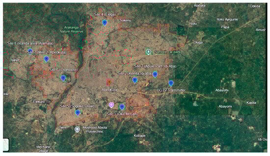
Figure 1. Location of the OGTV Transmitter and the eight receiving sites marked. Source: Google Earth (2025).

3.2. Assessment of Actual Path Loss at Chosen Sites Under Different Weather Conditions

Information on the transmitter’s operational parameters, specifically its output power and carrier frequency, was obtained from the DTTBS station. To estimate the effective radiated power, measurements of the signal level were performed at the transmitter’s base. The assessment of transmission performance at the receiver terminals was conducted using a digital signal strength meter to acquire Received Signal Strength data. Additionally, portable Global Positioning System (GPS) units were used to determine the elevation and geographic coordinates of each reception site with high precision.

Surface meteorological parameters, including ambient temperature, atmospheric pressure, and relative humidity, were simultaneously recorded at each measurement point using a compact wireless weather station. The integration of these environmental and radio-frequency datasets facilitated a comprehensive characterization of the propagation environment within the study area.

Data acquisition was conducted over a continuous twelve-month period, encompassing both wet and dry seasonal conditions. Measurements were systematically carried out seven times per day at 08:00, 10:00, 12:00, 14:00, 16:00, 18:00, and 20:00 h, thereby ensuring adequate temporal coverage of daily signal variations. This extensive dataset enabled a rigorous analysis of the interrelationship between signal behavior, meteorological conditions, and time of day. The actual path loss at each receiver location was derived as the difference between the transmitter’s nominal power and the corresponding measured RSS, thereby providing a reliable estimation of signal attenuation across the coverage area.

3.3. Modeling of Path Loss Prediction for DTTV Communication Link

A predictive model for estimating path loss within the study area was developed using multiple regression, accounting for distinct atmospheric conditions observed during the wet and dry seasons. To accurately compute surface radio refractivity values for each data collection site, the ITU-R refractivity equations (Equations (1)–(6)) were applied, incorporating real-time meteorological parameters such as temperature, humidity, and atmospheric pressure. The analysis was performed using MATLAB, which processed the signal data obtained from the transmitting base station under both seasonal conditions. This enabled a detailed evaluation of how environmental factors influence signal propagation. From the analyzed datasets, empirical path-loss models were derived using multiple regression, yielding season-specific equations that accurately predict radio signal attenuation across varying climatic and topographical conditions within the study area. These models aim to provide a comprehensive understanding of signal propagation and can be used for various applications [33,34,35,36].

Surface Radio Refractivity and Radio Signal

The radio refractivity parameter, $N$, describes the spatial and temporal variations in the index of refraction (n) of the air, which is frequently defined as (1):

$$N=\left(n-1\right){10}^6$$

(1)

According to ITU-R Recommendation P.453 (2003) [37], the surface radio refractivity $\left(N_s\right)$ is a dimensionless parameter that characterizes the refractive properties of the lower atmosphere and is primarily influenced by key meteorological variables such as atmospheric pressure (P) measured in hectopascals (hPa), temperature (T) expressed in Kelvin (K), and water vapor pressure (e) also in hectopascals (hPa). These parameters collectively determine how electromagnetic waves propagate through the troposphere by affecting the bending and attenuation of radio signals. The mathematical formulation describing the relationship between these atmospheric parameters and surface refractivity is presented in Equations (2)–(4), which serve as the foundational expressions for computing Nₛ at different data collection sites based on observed meteorological conditions:

$$N_s= {\displaystyle \frac{77.6}{T}}(P+4810{\displaystyle \frac{e}{T}})$$

(2)

with the dry term of radio refractivity $N_{dry}$ given by:

$$N_{dry}= 77.6{\displaystyle \frac{P}{T}}$$

(3)

and the wet term, $N_{wet}$ given by:

$$N_{wet}= 3.732\times {10}^5{\displaystyle \frac{e}{T^2}}$$

(4)

where

$$e={\displaystyle \frac{H{e}_s}{100}} \left(\mathrm{h}\mathrm{P}\mathrm{a}\right)$$

(5)

and

$$e_s=6.11 \mathrm{e}\mathrm{x}\mathrm{p}\left[{\displaystyle \frac{17.502t}{t+240.97}}\right]$$

(6)

Pressure and water vapor pressure decrease rapidly with increasing height, whereas temperature decreases slowly [33]. Dairo and Kolawole [34] emphasized that fluctuations in the surface radio refractivity gradient, determined by the surface refractivity (Nₛ), are crucial in defining the atmosphere’s refractive characteristics. These variations give rise to distinct atmospheric refractive conditions, including normal, sub-refractive, super-refractive, and ducting layers, each with a unique influence on the propagation of radio waves through the atmosphere. The occurrence of these refractive layers alters the bending, reflection, and attenuation of electromagnetic waves, thereby affecting signal strength and transmission range. Consequently, such atmospheric behaviors exert a profound impact on radio signal propagation across multiple frequency bands, notably the VHF, UHF, and microwave spectra. Understanding and modeling these refractive effects are therefore essential for optimizing the efficiency, performance, and reliability of terrestrial communication systems, particularly in regions where environmental and meteorological factors vary significantly [35,36].

3.4. Optimization of the Proposed Model

This research employed two optimization techniques to determine the best-fit pathloss model for the study area. Least Squares and Gradient Descent methods were used. The adoption of Least Squares (LS) as one of the optimization techniques in this study is justified by its statistical optimality and its long-standing acceptance in radio-propagation modeling. LS minimizes the sum of squared residuals between measured and predicted pathloss values, making it particularly suitable for RSS datasets where measurement noise is assumed to follow a Gaussian distribution. Its ability to provide a closed-form, unbiased, and analytically interpretable solution for linear or linearizable pathloss models such as the log-distance and COST-231 models makes it an essential baseline technique. LS therefore provides a mathematically rigorous and reproducible benchmark for assessing model performance in the study area.

Conversely, Gradient Descent (GD) was selected to complement LS because it is well-suited to optimizing nonlinear or complex pathloss formulations that cannot be solved analytically. GD iteratively minimizes the cost function, allowing the model parameters to adapt to irregular propagation environments shaped by obstacles, multipath, and shadowing effects. Its flexibility, scalability, and ability to navigate non-convex error surfaces make it advantageous for datasets with heterogeneous terrain or diverse measurement conditions. By employing both LS and GD, the study ensures robust parameter estimation and cross-validates results. It strengthens the reliability of identifying the most accurate pathloss prediction model for the study environment.

3.4.1. Least Squares Optimization Method

The conventional framework for statistical analysis entails the utilization of a dataset encompassing N pairs of observations, each denoted as ($Yi$, $Xi$). The fundamental objective is to construct a function that delineates the relationship between the dependent variable ($Y$) and the independent variable ($X$). In scenarios involving a single independent variable and a linear functional form, the prediction can be concisely expressed through the following Equation (7):

$$Y = {\beta }^0+ {\beta }^{1}X + \epsilon$$

(7)

The steps involved in the least squares method are as follows, and Figure 2 illustrates the technique’s flowchart.

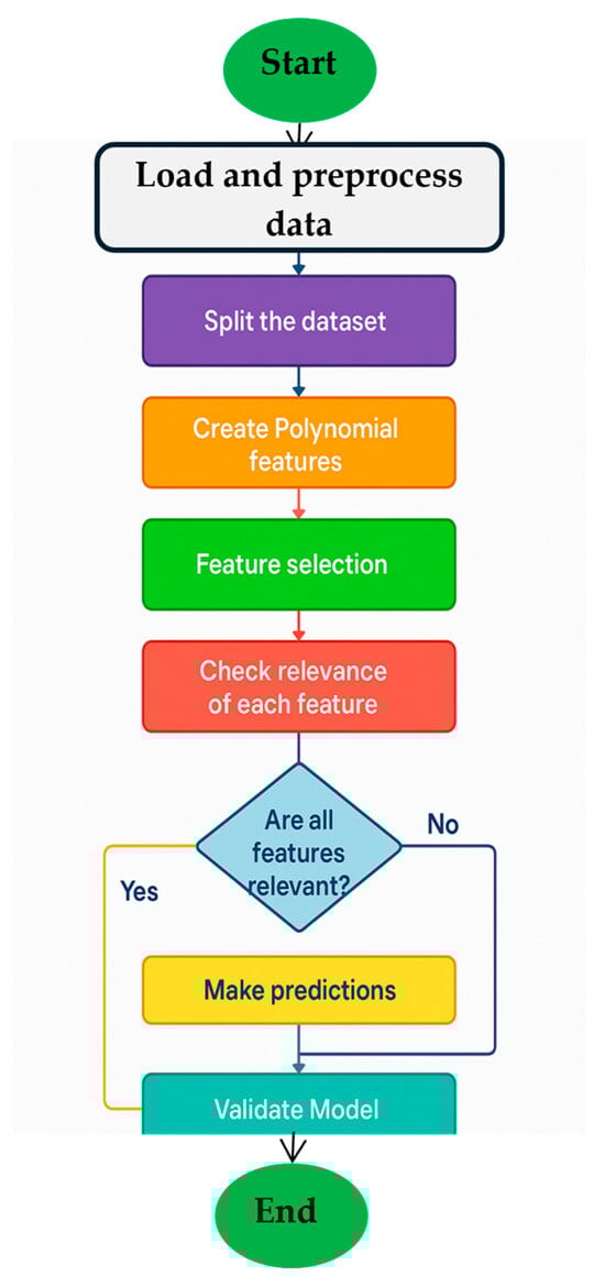
Figure 2. Flowchart for the Least Squares optimization method.

Step 1: Input Data

• Collect and preprocess the dataset:
• Load the dataset containing input features ($X$) and target values (y).
• Perform data preprocessing (cleaning, handling missing values, feature scaling, encoding categorical variables, etc.) if necessary.

Step 2: Model Representation

• Define the linear regression model:
• The linear regression model is represented as (8)

$$y={\beta }_0+{\beta }_1{x}_1+{\beta }_2{x}_2+{\beta }_3{x}_3+\dots +{\beta }_n{x}_n$$

(8)

where y is the target variable (dependent variable), $x_1, x_2, x_3\dots x_n$ are the input features (independent variables), ${\beta }_0$ is the intercept (bias term) and ${\beta }_1, {\beta }_2, {\beta }_3, \dots {\beta }_n$ are the coefficients of the input features.

Step 3: Model Training

• Calculate the model coefficients using the Normal Equation:

The coefficients (${\beta }_0, {\beta }_1, {\beta }_2\dots {\beta }_n$) can be calculated using the Normal Equation (9):

$$\beta ={\left(X^{T}X\right)}^{-1}{X}^{T}y$$

(9)

where $\beta$ is a vector of coefficients and $X$ is the matrix of input features.

Step 4: Model Prediction

• Use the trained model to make predictions:

Given new input feature values $x_1, x_2, x_3, \dots x_n$, one can predict the target variable by using the model as (10):

$$\widehat{y}={\beta }_0+ {\beta }_1{x}_1+ {\beta }_2{x}_2+ {\beta }_3{x}_3+\dots +{\beta }_n{x}_n$$

(10)

where $\widehat{y}$ is the predicted value.

Step 5: Model Evaluation

• Evaluate the model’s performance:

3.4.2. Gradient Descent Optimization Method

Gradient descent is a widely used optimization technique employed extensively in training neural networks and machine learning models. These models enhance their predictive accuracy through iterative exposure to training data. In gradient descent, the cost function serves as a crucial metric for assessing the model’s accuracy after each parameter update. The model systematically adapts its parameters to minimize the error, aiming to drive the cost function towards zero or to achieve convergence where it effectively becomes zero. When properly optimized, machine learning models can serve as highly effective tools across a range of applications in artificial intelligence (AI) and computer science.

To quantify the discrepancy between measured path loss values and model predictions, the Mean Squared Error (MSE) was used as the primary cost function. The MSE provides a smooth, differentiable error surface suitable for iterative minimization and is mathematically expressed as:

$$J(\theta )={\displaystyle \frac{1}{n}}{\sum }_{i=1}^n{\left({PL}_{measured, i}-{PL}_{predicted, i}\left(\theta \right)\right)}^2$$

(11)

where ${PL}_{measured}$ is the actual field-measured path loss, ${PL}_{predicted}\left(\theta \right)$ is the model estimate based on parameter vector $\theta$, and $n$ is the number of observations. The optimization objective is to determine the parameter set $\theta$ that minimizes $J\left(\theta \right)$, thereby ensuring maximum agreement between predicted and measured propagation behavior.

The gradient descent flowchart is illustrated in Figure 3.

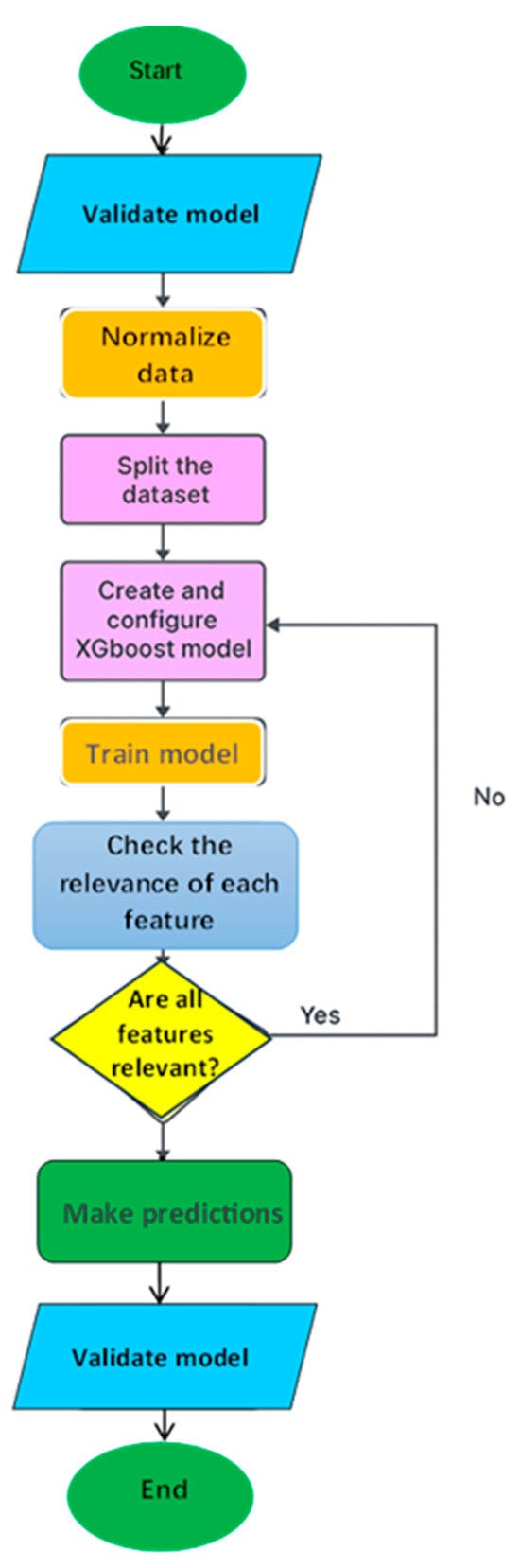
Figure 3. Flowchart of the gradient descent method.

Parameter Update Rule

Gradient Descent minimizes the cost function through iterative parameter updates in the direction of steepest descent of the error function, computed as:

$${\theta }^{(k+1)}={\theta }^{\left(k\right)}-\alpha \nabla J\left({\theta }^{\left(k\right)}\right)$$

(12)

where α denotes the learning rate and $\nabla J\left({\theta }^{\left(k\right)}\right)$ is the gradient of the cost function with respect to the model parameters at iteration k. The gradient indicates the degree to which each parameter contributes to the prediction error, allowing the algorithm to systematically reduce the discrepancy between the model and the observed signal behavior.

Convergence Criteria

To ensure reliable and stable parameter estimation, the following convergence criteria were applied:

-

Cost Function Stability:

$$\left|J\left({\theta }^{\left(k+1\right)}\right)-J\left({\theta }^{\left(k\right)}\right)\right|<{10}^{-6}$$

(13)

-

Parameter Update Magnitude:

$$\left|\left({\theta }^{\left(k+1\right)}\right)-\left({\theta }^{\left(k\right)}\right)\right|<{10}^{-5}$$

(14)

-

Maximum Iteration Cap:

A maximum of 1000 iterations was set to avoid divergence or excessive computation when the cost function landscape is irregular.

Parameter Tuning and Stability Considerations

The learning rate α plays a critical role in determining the stability and speed of convergence. An excessively high learning rate can cause overshooting or oscillation around the minimum, while a very small value results in slow convergence. In this study, α was tuned experimentally within the range:

$$\alpha \in [0.0001, 0.05]$$

to identify a value that ensured smooth descent of the cost function without instability. Feature scaling was applied to harmonize variables such as distance, elevation, and radio-refractivity, thereby preventing larger-scale variables from dominating the gradient and accelerating convergence.

Multiple parameter initializations were also tested to avoid convergence to suboptimal local minima, especially in the polynomial GD formulations.

3.5. Evaluation of the Proposed Method

Six commonly used statistical performance indicators were employed to evaluate the effectiveness and suitability of the proposed models for application within the study area. These include the Coefficient of Multiple Determination, Correlation Coefficient, Mean Squared Error, Root Mean Squared Error (RMSE), and Mean Absolute Error.

4. Results and Discussion

4.1. DTTV Transmission and Receiving Sites Parameters

The OGTV station, located within the Abeokuta metropolis and transmitting in the UHF band, was the site used for this research. The station transmits at 503.5 MHz, a frequency within the UHF band, which qualifies it for this study. The transmitter has a transmit power of 10 kW and a transmitter height of 304.8 m, while the receiver antenna height is 3 m. The receiving sites were selected along a contoured radius centered on the transmitter, with a spacing of 2 km between them. The longest distance from the transmitter to the farthest place in Abeokuta is 16.7 km; therefore, eight (8) receiving sites were used in this research.

The measurement points were positioned at distances ranging from 2 m to 16 m from the transmitter. The site located 2 m away (7°08′37″ N, 3°24′11″ N) had the highest elevation of 171 m, while the 4 m location (7°09′02″ N, 3°23′09″ N) recorded an elevation of 155 m. As the distance increased, elevation values varied across the sites, with the 6 m and 8 m locations at 66 m and 88 m, respectively. The 10 m site (7°06′43″ N, 3°20′10″ N) recorded the lowest elevation of 55 m, whereas the 12 m, 14 m, and 16 m locations had elevations of 69 m, 53 m, and 82 m, respectively. These variations in elevation and geographic positioning reflect the diverse topographical characteristics of the study area, which are essential for accurately assessing signal propagation behavior along different LOS distances from the transmitter.

4.2. Determination of Actual Loss Under Different Atmospheric Conditions via Measurements

At each of the eight designated receiving sites, the received signal strength (RSS) was simultaneously measured and recorded. The measurements were then processed to compute average RSS values, which were subsequently classified into wet and dry seasons based on their respective months of occurrence. The actual path loss for each location was derived as the difference between the transmitted and received signal levels. A comprehensive summary of the path loss values for both seasons is presented in Table 2.

Table 2. Actual path loss values measured at various locations.

Distance (km)	Transmitted Power (dB)	Measured Received Signal (dB)	Actual Path Loss (dB)	Measured Received Signal (dB)	Actual Path Loss (dB)
Wet Seasons				Dry Season
2	70	−11.9182	81.91817	−11.3235	81.32353
4	70	−21.7905	91.79048	−21.3198	91.31985
6	70	−30.1593	100.1593	−28.4542	98.45421
8	70	−34.5129	104.5129	−33.6579	103.6579
10	70	−36.8121	106.8121	−36.6338	106.6338
12	70	−41.3848	111.3848	−40.7344	110.7344
14	70	−44.2947	114.2947	−42.2088	112.2088
16	70	−47.1779	117.1779	−46.2135	116.2135

From a practical standpoint, the results carry significant implications for network engineers and planners. The ability of wireless networks to adapt to seasonal variations is crucial for maintaining reliable communication services. In regions with distinct wet and dry seasons, it is essential to anticipate and address fluctuations in signal propagation. From a practical standpoint, the results carry significant implications for network engineers and planners. The ability of wireless networks to adapt to seasonal variations is crucial for maintaining reliable communication services. In regions with distinct wet and dry seasons, it is essential to anticipate and address fluctuations in signal propagation.

The data in Table 2 reveal a notable disparity in measured path loss between the wet and dry seasons. Path loss tends to increase with increasing spatial separation between the transmitter and receiver. The observed data from the measurements clearly demonstrate that changes in weather conditions significantly impact received signal strength, subsequently influencing path loss. This variation in path loss can be attributed to the divergent weather conditions experienced during the wet and dry seasons. In a broad sense, the values exhibit a consistent pattern and trend across seasons. However, during the wet season, path loss is notably higher than in the dry season. This is due to the generally lower Received Signal Strength (RSS) values during the wet season, which, in turn, lead to higher path loss values at the same distances.

This indicates the adverse impact of weather conditions, such as rainfall and increased atmospheric moisture, on signal propagation. These conditions introduce additional signal absorption and scattering, leading to signal degradation. Conversely, during the dry season, signal propagation appears more efficient, as evidenced by higher RSS values at the same distances and, consequently, lower pathloss. These findings emphasize the importance of considering environmental factors when designing and planning wireless networks.

From a practical standpoint, the results carry significant implications for network engineers and planners. The ability of wireless networks to adapt to seasonal variations is crucial for maintaining reliable communication services. In regions with distinct wet and dry seasons, it is essential to anticipate and address fluctuations in signal propagation. This might involve adjusting transmitter power, optimizing antenna placement, or deploying additional infrastructure to mitigate signal degradation during adverse weather conditions.

The results presented in the study highlight the interplay between transmit power, received signal strength (RSS), and path loss. A consistent transmit power level of 70 dB serves as a reference point, facilitating path-loss computation by subtracting the measured RSS from it. As expected, path loss increases with distance from the transmitter, in accordance with the fundamental inverse-square law governing signal propagation. The consistent behavior observed in the study serves as a valuable reaffirmation of the basic principles underlying wireless communication.

4.3. Modeling of Pathloss for the Communication Link Across Both Wet and Dry Seasons

The yearly average values for the measured parameters over the period, representing the varying LOS distance from the transmitter at each location, are presented in Table 3. These data include Received Signal Strength (RSS), the corresponding Pathloss, the elevation of each receiving site, and the corresponding location-based Surface Radio Refractivity. It also shows the seasonal distribution of these parameters. The path loss models were developed using multiple regression analysis, considering the data collected during both the wet and dry seasons in Abeokuta. These models were designed to capture the relationship between various influencing factors and path loss. Equations (15) and (16) represent the proposed models for path loss during the wet and dry seasons, respectively. These equations are mathematical expressions that predict path loss based on specific parameters and conditions relevant to each season. The models consider environmental and atmospheric factors that affect signal propagation in Abeokuta across the different seasons.

$$M_{Wet} \left(\mathrm{dB}\right)=1073+2.125 D-0.098 E-2.601 N_s$$

(15)

$$M_{Dry} \left(\mathrm{d}\mathrm{B}\right)=2057.75+2.36 D-0.094 E-5.588 N_s$$

(16)

where D is the distance in km, E represents the receiving site’s elevation (m), and Surface radio refractivity based on location.

Table 3. Location-based Pathloss Measurement during Wet and Dry seasons.

Transmit Power (dB)	Receiver
	LOS Distance (km)	RSS (dB)	Pathloss (dB)	Elevation (m)	${\mathit{N}}_{\mathit{s}}$	RSS (dB)	Pathloss (dB)	Elevation (m)	${\mathit{N}}_{\mathit{s}}$
Wet Season						Dry Season
70	2	−11.9182	81.91817	171	375.7811	−11.3235	81.32353	171	351.2966
70	4	−21.7905	91.79048	155	375.7811	−21.3198	91.31985	155	351.2966
70	6	−30.1593	100.1593	66	376.8905	−28.4542	98.45421	66	352.0489
70	8	−34.5129	104.5129	88	375.7811	−33.6579	103.6579	88	351.8773
70	10	−36.8121	106.8121	55	377.7499	−36.6338	106.6338	55	352.2923
70	12	−41.3848	111.3848	69	377.7973	−40.7344	110.7344	69	352.8134
70	14	−44.2947	114.2947	53	377.7973	−42.2088	112.2088	53	352.8134
70	16	−47.1779	117.1779	82	377.7973	−46.2135	116.2135	82	352.8134

Equations (15) and (16) were used in the study to determine the expected path loss for the dry and wet seasons at different line-of-sight distances. The coefficient of determination (R²) and the correlation coefficient (R) were calculated by comparing the predicted path loss values with the measured path loss values. A comparison of the measured and model-predicted path loss values is shown in Table 4. This enables the evaluation of how well the models estimate path loss in various scenarios.

Table 4. Predicted vs. Measured Pathloss.

LOS Distance (km)	Measured Pathloss (dB)	Predicted Pathloss (dB)	Measured Pathloss (dB)	Predicted Pathloss (dB)
	Wet Season		Dry Season
2	81.91817	83.88921	81.918170	83.45275
4	91.79048	89.70816	91.790477	89.67822
6	100.1593	99.79943	100.15927	98.57567
8	104.5129	104.77823	104.51288	102.18131
10	106.8121	107.14245	106.81207	107.68894
12	111.3848	109.89625	111.38482	108.17695
14	114.2947	115.71520	114.29473	114.40243
16	117.1779	117.12137	117.17788	116.38970

During the wet season, the model’s predicted pathloss values exhibit some variation. At shorter distances, the model tends to overestimate pathloss, predicting a greater signal attenuation than the measured values. This overestimation may be due to localized factors or environmental variations that the model does not account for. As the distance increases, the gap between predicted and measured pathloss narrows, indicating that the model’s accuracy improves with greater line-of-sight (LOS) distance. However, the model again starts to overestimate pathloss at longer distances. This behavior may be influenced by factors such as terrain complexity or atmospheric conditions that the model does not fully account for. Similarly, the model’s predictions demonstrate some variability during the dry season. At shorter distances, the model tends to overestimate pathloss, consistent with the pattern observed in the wet season.

As the distance increases, the model’s predictions become more accurate and closely align with the measured pathloss values. Nonetheless, the model continues to overestimate pathloss at longer distances. These results underscore the importance of accurate pathloss predictions for effective network planning and infrastructure deployment. Factors such as terrain variations, atmospheric conditions, and local environmental characteristics can introduce complexities that compromise the accuracy of pathloss predictions. Therefore, further adjustments and the inclusion of additional factors may be necessary to improve the model’s ability to predict pathloss across a broader range of conditions and distances.

The coefficients of correlation and multiple determination were computed for both the wet and dry seasons to assess the goodness-of-fit of the developed models. These statistical indicators provide valuable insight into the models’ performance by quantifying the strength and direction of the linear relationship between the predicted and observed values, as well as the proportion of variance in the measured data that the models can explain. Higher R and R² values imply stronger correlation and better predictive capability, indicating that the model effectively captures the underlying signal propagation behavior across varying seasonal conditions. ${PL}_{wet}$ has a $R$ and $R^2$ value of 0.993 and 0.988, respectively, while ${PL}_{dry}$ has 0.987 and 0.977, both for $R$ and $R^2$ respectively. This suggests that the model provides a good fit for the data and effectively explains the variations in the dependent variable. The exceptionally high correlation coefficients are noteworthy. ${PL}_{wet} \left(\mathrm{d}\mathrm{B}\right)$ demonstrates a robust correlation of 0.993, while ${PL}_{dry} \left(\mathrm{d}\mathrm{B}\right)$ follows closely with a correlation coefficient of 0.987. Such high correlation coefficients affirm the models’ reliability in estimating signal strength, even under changing environmental conditions between the wet and dry seasons.

Furthermore, multiple regression coefficients are impressively close to 1, indicating that the models are excellent fits for the data. ${PL}_{wet} \left(\mathrm{d}\mathrm{B}\right)$ boasts a coefficient of 0.988, and ${PL}_{dry} \left(\mathrm{d}\mathrm{B}\right)$ exhibits a strong fit during the dry season, with a coefficient of 0.977. These coefficients underline the models’ ability to explain and predict variances in signal behavior effectively, while considering the specified independent variables $(D, E, N_S ).$ The high correlation coefficients and strong multiple regression coefficients indicate the robustness and accuracy of these predictive models. They provide dependable tools for estimating and predicting signal strength during both wet and dry seasons, ensuring the consistency and reliability of wireless communication services.

4.3.1. Comparison of the Proposed Models with Other Empirical Models

The models developed for both the wet and dry seasons were evaluated against three well-established empirical models: Hata, Okumura, and ECC-33 to assess their predictive accuracy and contextual applicability. The comparative analysis, illustrated in Figure 3, shows that the Path Loss values estimated using the Hata and ECC-33 models were considerably higher than those predicted by the proposed models. This pronounced overestimation indicates that these traditional empirical models are unsuitable for accurate Path Loss prediction within the study area. The observed discrepancies may be attributed to variations in terrain configuration, climatic conditions, and propagation environments between the original datasets used to develop these models and the current study environment. These differences highlight the inherent limitations of applying generalized propagation models to regions with distinct environmental and meteorological characteristics.

The superior performance of the proposed models can be attributed to their calibration using locally measured propagation data, which enabled the integration of site-specific environmental parameters. Unlike conventional empirical models, which were primarily designed for temperate, urbanized environments, the proposed models were tailored to represent the unique climatic, topographical, and vegetative features of the study area. This contextual tuning enhanced their ability to accurately reflect the influence of factors such as terrain elevation, atmospheric refractivity, relative humidity, and seasonal variability on signal attenuation. As a result, the developed models demonstrated higher correlation with measured data and lower prediction errors, confirming their reliability, precision, and robustness for radio propagation analysis in tropical regions with similar environmental settings. Further statistical analyses are presented in Table 5, providing additional insights into the model comparisons.

Table 5. Statistical analyses for the Model comparison.

Models	Pathloss Mean Value (dB)	RMSE (dB)	MAE (dB)
Hata	164.5461	63.0454	61.0399
Okumura	97.9386	8.5631	7.6510
ECC-33	38.9562	65.1343	64.5501
${PL}_{wet}$	103.5062	1.2633	0.9968
${PL}_{dry}$	102.5682	1.8184	1.5678

Figure 4 illustrates the contrasting trends in Path Loss between the Okumura model and the proposed models as the distance from the transmitter increases. Notably, the Okumura model shows a gradual, relatively modest rise in Path Loss with distance, suggesting a tendency to underestimate the rate of signal attenuation along the propagation path. This behavior can be attributed to the empirical nature of the model, which was initially developed under different environmental and frequency conditions, particularly in urban settings with moderate terrain variation. In contrast, the proposed models exhibit a more pronounced and realistic increase in Path Loss with distance, showing stronger agreement with the measured field data. This pattern suggests that the proposed models more accurately capture the influence of environmental and topographical factors, such as terrain elevation, vegetation density, and atmospheric refractivity, which play a critical role in radio signal propagation within the study environment.

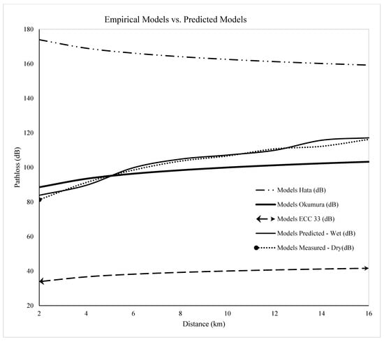
Figure 4. Pathloss from the Empirical vs. Predicted Model.

The observed trend thus reinforces the reliability and predictive capability of the proposed models compared to conventional empirical formulations. In contrast, the proposed models exhibit a more pronounced increase in Pathloss with increasing distance. This divergence in pathloss behavior can be attributed to the crowded environmental conditions of the study area, characterized by high-rise buildings and densely populated areas. As a result, Line-of-Sight (LOS) communication between transmitting and receiving antennas is often obstructed. Consequently, the received signal predominantly comprises reflected or scattered multipath components. This situation is common among most subscribers in these areas, leading to the observed Pathloss patterns. The proposed models exhibit variations with distance, characterized by regular crests and troughs that reflect the impact of location-specific tropospheric parameters.

In both seasons, the Okumura model exhibits the closest agreement with the proposed models, as indicated by the three indices in Table 5. This suggests that the Okumura model provides results that are more consistent with the proposed models than other empirical models. The Mean Pathloss represents the average pathloss values predicted by each model. A lower Mean Pathloss typically indicates underestimation of pathloss, while a higher value suggests overestimation. In this comparison, the ECC-33 model stands out with the lowest Mean Pathloss of 38.9562 dB, suggesting it generally underestimates pathloss relative to the other models. Conversely, the Hata model has the highest Mean Pathloss at 164.5461 dB, indicating that it consistently overestimates pathloss. The ${PL}_{wet}$ and ${PL}_{dry}$ models fall in between, with values close to each other. These findings suggest that the ECC-33 model may yield more optimistic predictions, whereas the Hata model is more conservative.

The RMSE measures the overall error of each model’s predictions, with lower values indicating greater accuracy. In this case, Okumura, ${PL}_{wet}$, and ${PL}_{dry}$ models exhibit the lowest RMSE values, indicating that they offer more accurate predictions than the Hata and ECC-33 models. The ECC-33 model has the highest RMSE, suggesting that its predictions differ significantly from the measured data. For both seasons, the ${PL}_{wet}$ and ${PL}_{dry}$ models in the research areas exhibited slightly higher values than the conventional Okumura-Hata model. The difference in RMSE values, about 7 dB, between the Okumura model and the proposed models is noteworthy. It should not be overlooked, especially when considering the potential implications for minimizing coverage failures, particularly in digital channels. This suggests that the Okumura model underestimated the channel path losses at the study locations. This is a crucial metric because it highlights the models’ precision and their ability to align with real-world observations.

The MAE measures the average magnitude of the errors between predicted and actual values; lower MAE values indicate more accurate predictions. Once again, Okumura, ${PL}_{wet}$, and ${PL}_{dry}$ models present the lowest MAE values, signifying more accurate predictions. The ECC-33 model has the highest MAE, suggesting larger prediction errors. MAE is vital for understanding the practical implications of the models’ accuracy in real-world applications.

The results obtained from the performance evaluation clearly demonstrate that the Okumura, ${PL}_{wet}$, and PL_dry models yield more accurate and reliable path loss predictions compared to the Hata and ECC-33 models. This outcome can be attributed to the ability of these models, particularly the proposed seasonal variants (${PL}_{wet}$ and ${PL}_{dry}$), to better account for the local propagation conditions in Abeokuta, which is characterized as a partially urban and suburban environment. In such mixed-terrain regions, the predictive accuracy of empirical models developed for strictly urban or rural settings often deteriorates, resulting in deviations from acceptable prediction ranges. The comparative assessment revealed that while the Hata, ECC-33, and Okumura models produced path loss values that were slightly outside the optimal range, the ${PL}_{wet}$ and ${PL}_{dry}$ models-maintained Root Mean Square Error (RMSE) values well within the permissible 0–6 dB threshold.

Although the Okumura model remains one of the most widely recognized and accepted empirical models for radio propagation analysis, often serving as a reference benchmark for developing and validating new path loss prediction techniques [37,38], it exhibits a fundamental limitation: its inability to incorporate tropospheric parameters such as refractivity, temperature, pressure, and humidity gradients. These parameters play a significant role in modifying radio wave propagation, especially in tropical regions like Abeokuta, where seasonal variations in atmospheric conditions substantially influence signal attenuation and propagation behavior. The exclusion of such parameters therefore constrains the Okumura model’s adaptability to local climatic and environmental variations, underscoring the need to develop a more robust, region-specific path-loss model.

The analysis presented in this study addresses this limitation by introducing two new empirical models; ${PL}_{wet}$ and ${PL}_{dry}$, that explicitly consider the influence of tropospheric parameters under varying meteorological conditions. The evaluation of these models against measured data revealed superior predictive accuracy, as evidenced by lower RMSE values than those of existing models. Significantly, the RMSE values of both proposed models fall within the study’s acceptable limit of 6 dB [39,40], confirming their reliability for path loss estimation across the study area.

4.3.2. Optimization of the Model

Two techniques were used to optimize the data. Gradient Descent Optimization (GDO) and Least Squares Optimization (LSO). Equations (17)–(20) are the optimization models for GDO and LSO for both Wet and Dry seasons. Equations (17) and (18) are linear, while (19) and (20) are polynomial.

$$\begin{array}{cc}{M}_{\left(wet-GD\right) }\left(\mathrm{d}\mathrm{B}\right)=& P_T-(-33.5494+0.0174N_s+0.0157P_V+0.2865T+0.146H_R-8.6674D+3.5067E\hfill \\ & + 0.6386P\hfill \end{array}$$

(17)

$$\begin{array}{cc}{M}_{\left(dry-GD\right)} \left(\mathrm{d}\mathrm{B}\right)=& P_T-(-32.5602-0.1281N_s-0.2093P_V+0.0334T+0.2199H_R-8.3697D+3.0653E\hfill \\ & + 0.0939P\hfill \end{array}$$

(18)

$$\begin{array}{cc}{M}_{\left(wet-LS\right)} \left(\mathrm{d}\mathrm{B}\right)=& P_T-(-37.4776+0.1702N_s-0.1722H_R-0.0104D{N}_s-0.0007E{N}_S-5.894\ast {10}^{-5}TP\hfill \\ & + 0.0097D{H}_R+0.0007E{H}_R+0.0664D^2+0.0011E^2 \hfill \end{array}$$

(19)

$$\begin{array}{cc}{M}_{(dry-LS)} \left(\mathrm{d}\mathrm{B}\right)=& P_T-(-28.9028-0.0680N_s+0.1825H_R-3.5111D+0.0005T{N}_S+0.0108N_S{H}_R\hfill \\ & - 0.0393P_V{H}_R-0.0023{H_R}^2-0.0031{PH}_R+0.1100D^2-0.0084DE+0.0002E^2 \hfill \end{array}$$

(20)

where $P_T$ is the Transmit Power (dB), $N_s$ is the Surface radio refractivity for a specific location (N-unit), $H_R$ represents the Relative Humidity, $D$; the Line-of-Sight Distance (km), $P_V$; the Vapor pressure, $P$ represents the Pressure (mbar) while $E$ represents the Elevation (m). Table 6 gives the predicted pathloss using GDO and LSO for both wet and dry seasons.

Table 6. Predicted Pathloss using GDO and LSO for both Wet and Dry seasons.

Distance	Wet Season		Dry Season
	GDO Prediction (dB)	LSO Prediction (dB)	GDO Prediction (dB)	LSO Prediction (dB)
2	84.73957	81.09353	84.17079	82.85834
4	88.86164	89.14757	88.99502	91.62421
6	100.43800	96.91941	98.76676	97.43077
8	102.74250	102.25580	101.08010	104.44500
10	107.81000	104.69090	107.11000	107.06730
12	110.75840	109.29140	109.75030	111.12380
14	115.86470	111.12720	114.68200	112.62110
16	117.27550	115.03220	116.19350	117.11700

As shown in Table 6 and Figure 5 and Figure 6, the path loss for the optimized models increases with distance, consistent with the pre-optimized path loss. It was also observed to follow a similar undulating trend with distance, with typical crests and troughs, unlike the Okumura model, which showed a smooth, incremental curve. Physical observation indicates that the Okumura model is not a good fit for the study area, as the curve is far from all the prediction models and the measured pathloss. However, the performance metrics for each model are presented in Table 7.

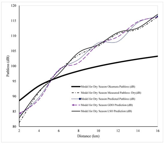
Figure 5. Comparison of the Pathloss of the various Models for the Dry season.

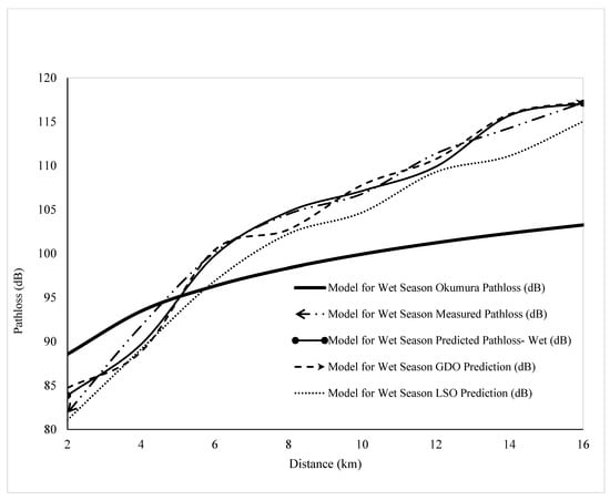
Figure 6. Comparison of the Pathloss of the various Models for the Wet season.

Table 7. Performance Metrics for the evaluation.

Metrics	Predicted Model Before Optimization (dB)	After Optimization (dB)		Predicted Model Before Optimization (dB)	After Optimization (dB)
	Wet Season			Dry Season
		GDO	LSO		GDO	LSO
RMSE	1.2633	1.7180	2.4180	1.8184	2.8298	1.1884
Correlation Coefficient	0.9935	0.9835	0.9934	0.9884	0.9808	0.9942
Coefficient of Multiple Determination	0.9871	0.9673	0.9868	0.9771	0.9620	0.9883
MAE	0.9968	23.6132	46.7750	1.5678	1.6472	0.7692
MSE	1.5959	2.9517	5.8469	3.3066	8.0075	1.4124

Table 7 presents a detailed comparison of the variation and behavior of predicted path loss values before optimization, the measured path loss, and the expected path loss after optimization. Comparing these datasets enables a critical evaluation of the efficiency, adaptability, and reliability of the proposed propagation models under varying environmental and meteorological conditions. By examining the models’ performance before and after optimization, as well as across different seasons, a more comprehensive understanding of their predictive accuracy and generalization capabilities is achieved.

In the wet season, the ${PL}_{wet}$ model demonstrates an exceptional level of predictive accuracy. This is evidenced by its remarkably low Root Mean Square Error (RMSE) of 1.2633, indicating minimal deviation between the predicted and measured signal strengths. Such a low RMSE signifies that the model is highly proficient in reproducing the observed propagation characteristics of the digital terrestrial television signal during periods of high atmospheric moisture content. Additionally, ${PL}_{wet}$ maintains a strong positive correlation with the measured field data, as reflected by its high correlation coefficient (r = 0.9935). This strong linear relationship reveals that the model’s predicted values closely align with the empirical observations, confirming its robustness and suitability for wet-season conditions.

Furthermore, the Mean Absolute Error (MAE) of 0.9968 was obtained for the ${PL}_{wet}$ model reveals its ability to maintain consistent prediction accuracy across multiple measurement points. The low MAE implies that the model’s estimates of received signal strength deviate only slightly from the actual field measurements, making it a highly dependable model for wet-season propagation prediction. The superior performance of ${PL}_{wet}$ can be attributed to its incorporation of atmospheric variables, such as increased humidity, an elevated refractive index, and enhanced surface moisture, which typically prevail during the wet season and strongly influence radio wave propagation. These environmental parameters often contribute to multipath effects and refractive bending of radio signals, which the model effectively captures through its parameterization.

In contrast, the optimized models, namely ${PL}_{Wet-GD}$ (Gradient Descent optimized) and ${PL}_{wet-LS}$ (Least Squares optimized), do not exhibit comparable levels of accuracy under wet-season conditions. Both models recorded relatively higher RMSE values, lower correlation coefficients, and significantly larger MAE values compared to ${PL}_{wet}$. This decline in performance suggests that the optimization procedures applied to the base models may have led to overfitting or parameter adjustments that did not adequately account for the high atmospheric variability and signal scattering associated with wet-season propagation. Consequently, rather than improving predictive reliability, the optimization process appears to have reduced model adaptability to the complex refractive environment characteristic of the wet season.

The unusually high MAE (23.6132) observed for the Gradient Descent optimized model in the wet season is due to convergence instability caused by the algorithm’s sensitivity to the learning rate and the error surface of the propagation model. The wet-season dataset exhibited higher variability and noise due to atmospheric moisture fluctuations, making the cost function less smooth and causing the model to overshoot the optimal parameters rather than settling at a minimum. As a result, the algorithm converged to a sub-optimal solution, leading to exaggerated prediction errors. At the same time, the Least Squares method, being analytically stable and not iterative, was unaffected by such instability.

The results, therefore, highlight that while optimization techniques can be effective in refining model parameters, their success depends heavily on prevailing climatic and topographical conditions. The behavior of the optimized models during the wet season suggests that optimization algorithms calibrated under relatively stable atmospheric conditions may fail to generalize well in dynamic environments characterized by high humidity, frequent precipitation, and variable refractivity gradients. This observation underscores the importance of context-specific model tuning and the inclusion of meteorological parameters during model calibration to enhance overall predictive accuracy. The performance of the ${PL}_{wet}$ model shows that the model is the best fit for the Wet season among the three models in comparison, while the M_GDO did better among the two optimization techniques.

However, the dynamics of model performance exhibit a notable shift during the dry season, where the optimized model, $M_{LS}$, emerges as the most accurate and reliable predictor of signal attenuation. The $M_{LS}$ model achieves the lowest Root Mean Square Error (RMSE) value of 1.1884, outperforming the unoptimized dry-season model, ${PL}_{dry}$, which records a higher RMSE of 1.8184. This substantial reduction in RMSE reflects a marked improvement in the model’s ability to reproduce measured signal strengths with minimal deviation. Moreover, $M_{LS}$ demonstrates a strong positive linear correlation with the observed data, as indicated by its correlation coefficient (r = 0.9942), further confirming the close agreement between its predictions and the empirical measurements.

In addition, ${PL}_{Dry-LS}$ records a Mean Absolute Error (MAE) of 0.7692, the lowest among all tested models during the dry season. This result indicates that the optimized model consistently delivers highly accurate estimates of received signal strength across the measurement points, thereby demonstrating its robustness and reliability under the relatively stable atmospheric conditions that prevail during the dry season. The superior performance of ${PL}_{Dry-LS}$ can be attributed to reduced atmospheric water vapor content, lower refractive index variability, and the dominance of direct line-of-sight propagation during this period, which collectively provide a more predictable propagation environment that aligns well with the assumptions underlying least-squares optimization.

These findings highlight the season-dependent behavior of path loss models and the crucial role of environmental variability in determining model suitability, in line with [41]. While the original models exhibit exceptional accuracy during the wet season when atmospheric moisture and refractive gradients significantly influence signal propagation, the optimized models, particularly ${PL}_{Dry-LS}$, demonstrate superior adaptability during the dry season, when stable atmospheric conditions and minimal multipath effects primarily govern propagation. This contrast emphasizes that the optimization process does not universally enhance performance but rather interacts with environmental parameters in a context-dependent manner.

The analysis, therefore, explains the necessity of seasonally adaptive modeling approaches for accurate prediction of radio signal behavior in tropical regions. Selecting or tuning a model according to prevailing meteorological conditions ensures that prediction accuracy, network reliability, and overall communication quality are maintained throughout the year. From a practical standpoint, these results provide critical insights for network planning and optimization, particularly for digital terrestrial television and other wireless communication systems operating in regions with pronounced climatic variability.

Ultimately, the study confirms that while the developed empirical models are effective in specific seasonal contexts, integrating optimization techniques, especially those employing least-squares adjustment, can significantly enhance predictive performance under specific environmental regimes. This adaptive approach contributes to more reliable network design, improved spectrum management, and the assurance of consistent service quality across both wet and dry seasonal conditions in the study area.

4.4. Model Generalization and Validation

Ensuring that the developed path-loss models remain reliable beyond the specific measurement locations used for training is a critical requirement for their applicability in real-world network planning. To assess the generalization capability of the optimized models, validation was performed using an independent dataset collected from measurement routes that were not included during the parameter estimation stage. This approach helps determine whether the optimized parameters truly capture the underlying propagation characteristics of the environment rather than overfitting to the training data.

During validation, each model’s predictions were computed using the independently measured RSS and meteorological variables, and their performance was evaluated using the same error metrics applied during training (MAE, RMSE, and correlation coefficient). Models that generalize well typically maintain low error values and consistent prediction trends across both datasets. In this study, the generalized performance of the optimized dry-season models remained stable across the independent dataset, reflecting their robustness under relatively uniform atmospheric conditions. However, the wet-season models exhibited noticeable performance degradation, highlighting the influence of rapidly varying atmospheric refractivity and moisture content on model stability. This observation underscores the need for incorporating more dynamic or season-aware modeling strategies for propagation environments characterized by high variability.

5. Conclusions

A crucial decision for DTTV communication in the UHF band is choosing the appropriate radio propagation model. A model like this helps explain how the signal behaves as it travels from the transmitter to the receiver. It successfully creates a relationship between the route loss sustained and the distance between the transmitter and receiver. In turn, this path loss is influenced by multiple essential factors, such as the operational frequency, the state of the atmosphere, the distinction between indoor and outdoor settings, the environmental conditions (urban, rural, dense urban, suburban, open, forest, sea, etc.), and, most importantly, the distance between the transmitter and the receiver. Making an informed decision about the appropriate propagation model is essential for optimizing signal reliability and quality in DTTV communication.

The study collected data from eight strategically selected reception locations, where both location-specific meteorological parameters and Received Signal Strength measurements were obtained. Based on the average measurement values, the dataset was categorized into two distinct meteorological conditions, representing periods of low and high atmospheric moisture content. The actual path loss at each location was determined by subtracting the measured RSS from the transmitted power. This approach provided a realistic representation of signal attenuation under varying environmental conditions. In assessing the predictive performance of the three empirical models, the analysis revealed that the Okumura model exhibited the closest agreement with the measured path loss values across multiple performance indicators. This finding indicates that the Okumura model provides a more accurate representation of propagation characteristics in the study environment than the Hata and ECC-33 models. The model’s relative accuracy may be attributed to its empirical foundation, which accounts for a broader range of propagation scenarios, including semi-urban and irregular terrains similar to those encountered in the study area.

Data optimization was carried out using a Machine learning algorithm. Two techniques (Gradient Descent and Least Squares Optimization) were used to analyze the data. For each method, separate models were developed for the dry and wet seasons, and six performance metrics were used to evaluate these models. For the wet season, the unoptimized model provided the best fit. In contrast to the dry season, the Least Squares Optimization Technique best predicted the pathloss for DTTV in the study area.

The study’s main limitation is its reliance on measurements from only eight reception locations, which, although strategically selected, may not fully capture the spatial and environmental variability across the broader service area. In addition, the analysis focused solely on three empirical pathloss models and two optimization techniques, potentially overlooking contemporary or hybrid models that might perform better in complex terrain or under varying climatic conditions. Future research should expand the measurement campaign to include more diverse locations, incorporate higher-resolution terrain and clutter data, and evaluate a broader range of propagation models, including machine-learning-based or hybrid deterministic approaches. Further extensions could also examine long-term seasonal variations, integrate digital terrain models, and explore adaptive optimization methods to enhance the accuracy and generalizability of DTTV pathloss predictions.

References

- Igwe, K.C.; Oyedum, O.D.; Aibinu, A.M.; Ajewole, M.O.; Moses, A.S. Application of artificial neural network modeling techniques to signal strength computation. Heliyon 2021, 7, e06047. [Google Scholar] [CrossRef]
- Ribeiro, L.C.; Kürner, T. Path Loss Measurements and Models at 300 GHz in an Industrial Environment. In Proceedings of the 2025 19th European Conference on Antennas and Propagation (EuCAP), Stockholm, Sweden, 30 March–4 April 2025; pp. 1–5. [Google Scholar] [CrossRef]
- Rappaport, T.S. Free Space Propagation Model. In Wireless Communications Principles and Practice, 2nd ed.; Prentice Hall: Upper Saddle River, NJ, USA, 2002; pp. 107–109. [Google Scholar]
- Wang, Y.; Fu, J.; Cao, Y. A weighted hybrid indoor positioning method based on path loss exponent estimation. Ad Hoc Netw. 2025, 166, 103684. [Google Scholar] [CrossRef]
- Zhang, S.; Wang, H.; Shen, Z.; Chang, C.; Li, X. Transmitter Location-Independent Path Loss Exponent Estimation via RSS measurements with Shadowing Effect. IEEE Antennas Wirel. Propag. Lett. 2025, 24, 2864–2868. [Google Scholar] [CrossRef]
- Siaw, N.J. A Proposed Implementation of Digital Terrestrial Television (DTT): Case Study: Ashanti Region-Ghana. Ph.D. Thesis, Kwame Nkrumah University of Science and Technology, Kumasi, Ghana, 2013. [Google Scholar]
- Tsoulos, G.; Athanasiadou, G.; Zarbouti, D.; Nikitopoulos, G.; Tsoulos, V.; Christopoulos, N. 5G and 4G in the Field: Performance Assessment through Trials. In Proceedings of the 2024 Panhellenic Conference on Electronics & Telecommunications (PACET), Thessaloniki, Greece, 28–29 March 2024; pp. 1–4. [Google Scholar] [CrossRef]
- Rochman, M.I.; Ye, W.; Zhang, Z.-L.; Ghosh, M. A Comprehensive Real-World Evaluation of 5G Improvements Over 4G in Low- and Mid-Bands. IEEE Trans. Cogn. Commun. Netw. 2025, 11, 1427–1441. [Google Scholar] [CrossRef]
- Huang, J.; Qian, F.; Gerber, A.; Mao, Z.M.; Sen, S.; Spatscheck, O. A close examination of performance and power characteristics of 4G LTE networks. In Proceedings of the 10th International Conference on Mobile Systems, Applications, and Services (MobiSys’12), Low Wood Bay Lake, UK, 25–29 June 2012; Association for Computing Machinery: New York, NY, USA, 2012; pp. 225–238. [Google Scholar] [CrossRef]
- Östlin, E.; Zepernick, H.J.; Suzuki, H. Macrocell path-loss prediction using artificial neural networks. IEEE Trans. Veh. Technol. 2010, 59, 2735–2747. [Google Scholar] [CrossRef]
- Isabona, J.; Srivastava, V.M. Hybrid neural network approach for predicting signal propagation loss in urban microcells. In Proceedings of the 2016 IEEE Region 10 Humanitarian Technology Conference (R10-HTC), Agra, India, 21–23 December 2016; pp. 1–5. [Google Scholar]
- Okoro, O.N.; Agbo, G.A. The effect of variation of meteorological parameters on the tropospheric radio refractivity for Minna. Glob. J. Sci. Front. Res. Phys. Space Sci. 2012, 12, 4–6. [Google Scholar]
- Akinbolati, A.; Ajewole, M.O.; Adediji, A.T.; Ojo, J.S. The influences of meteorological parameters on digital terrestrial television (DTT) signal in the tropics. Int. J. Digit. Inf. Wirel. Commun. 2017, 7, 161–172. [Google Scholar] [CrossRef]
- Ajewole, M.O.; Akinbolati, A.; Adediji, A.T.; Ojo, J.S. Precipitation effect on the coverage areas of terrestrial UHF television stations in Ondo state, Nigeria. Int. J. Eng. Technol. 2014, 4, 524–535. [Google Scholar]
- Pawar, S.; Venkatesan, M. A novel pathloss prediction and optimization approach using deep learning in millimeter wave communication systems. e-Prime Adv. Electr. Eng. Electron. Energy 2024, 9, 100737. [Google Scholar] [CrossRef]
- Akinbolati, A.; Ajewole, M.O. Investigation of path loss and modeling for digital terrestrial television over Nigeria. Heliyon 2020, 6, e04101. [Google Scholar] [CrossRef]
- Edwan, T.A.; Tahat, A. On optimising pixel arrangement in tabular-data transformation for CNN-based path-loss prediction: A single-image, multi-frequency approach. Phys. Commun. 2025, 72, 102720. [Google Scholar] [CrossRef]
- Sharma, H.; Sahu, S.; Sharma, S. Enhanced Cost231 W.I. Propagation Model in Wireless Network. Int. J. Comput. Appl. 2011, 19, 36–42. [Google Scholar] [CrossRef]
- Zhang, Y.; Wen, J.; Yand, G.; He, Z.; Luo, X. Air-to-air Path Loss based on Machine Learning methods in Urban Environments. Wirel. Commun. Mob. Comput. 2018, 2018, 8489326. [Google Scholar] [CrossRef]
- García, N.A.; Pinto, A.D.; Torres, J.M.; Rengel, J.; Rujano, L.M.; Camargo, N.R.; Donoso, Y. Improved ITU-R model for digital terrestrial television propagation path loss prediction. Electron. Lett. 2017, 53, 832–834. [Google Scholar] [CrossRef]
- Bakare, B.I.; Ekeocha, A. A critical review of Digital Terrestrial Television broadcasting in Nigeria. EJECE J. Electr. Comput. Eng. 2018, 2, 7–10. [Google Scholar] [CrossRef]
- Bendov, O. Interference to UHF-DTTV Channels by Unlicensed Devices. IEEE Trans. Broadcast. 2006, 52, 443–449. [Google Scholar] [CrossRef]
- Ojo, S.; Imoize, A.; Alienyi, D. Radial basis function neural network path loss prediction model for LTE networks in multitransmitter signal propagation environments. Int. J. Commun. Syst. 2021, 34, e4680. [Google Scholar] [CrossRef]
- Moraitis, N.; Tsipi, L.; Vouyioukas, D.; Gkioni, A.; Louvros, S. Performance evaluation of machine learning methods for path loss prediction in rural environment at 3.7 GHz. Wirel. Netw. 2021, 27, 4169–4188. [Google Scholar] [CrossRef]
- Nasir, F.; Quadri, R.A.; Imam-Fulani, Y.O.; Kayode, S.A.; Abubakar, A.; Abdulkarim, A.O.; Haruna, C.; Olugbenga, A.S.; Lukman, A.O.; Salisu, G.; et al. ANN-based model for multiband path loss prediction in built-up environments. Sci. Afr. 2022, 17, e01350. [Google Scholar] [CrossRef]
- Ukatu, I.; Meneya, N. Performance analysis of path loss models for digital terrestrial transmission in urban and rural environment. Indian J. Eng. 2022, 19, 410–414. [Google Scholar]
- Adeyemi, J.; Surajudeen-Bakinde, N.; Nasir, F.; Ayeni, A.; Obiyemi, O.; Bello, O. Performance Analysis of Empirical Path Loss Models in VHF & UHF Bands. In Proceedings of the 6th International Conference on Information and Communication Systems (ICICS 2015), Amman, Jordan, 7–9 April 2015. [Google Scholar] [CrossRef]
- Jawhly, T.; Tiwari, R.C. The special case of Egli and Hata model optimization using least-square approximation method. SN Appl. Sci. 2020, 2, 1296. [Google Scholar] [CrossRef]
- Jo, H.S.; Park, C.; Lee, E.; Choi, H.K.; Park, J. Path Loss Prediction Based on Machine Learning Techniques: Principal Component Analysis, Artificial Neural Network and Gaussian Process. Sensors 2020, 20, 1927. [Google Scholar] [CrossRef] [PubMed] [PubMed Central]
- Sathaporn, P.; Thanadol, T.; Bundit, R. Evaluation of DTTV Transmission for SFN with Minimum Threshold in Thailand. Wirel. Pers. Commun. 2020, 115, 2819–2832. [Google Scholar] [CrossRef]
- Isabona, J.; Imoize, A.L. Terrain-based adaption of propagation model loss parameters using non-linear square regression. J. Eng. Appl. Sci. 2021, 68, 33. [Google Scholar] [CrossRef]
- Hoiberg, D.H. (Ed.) Abeokuta. In Encyclopædia Britannica. I: A-ak Bayes, 15th ed.; Encyclopaedia Britannica Inc: Chicago, IL, USA, 2010; p. 27. [Google Scholar]
- Ayantunji, B.G.; Okeke, P.N.; Urama, J.O. Diurnal and seasonal variation of Surface Refractivity over Nigeria. Prog. Electromagn. Res. B 2011, 30, 201–222. [Google Scholar] [CrossRef]
- Dairo, O.F.; Kolawole, L.B. Statistical analysis of radio refractivity gradient of the rainy-Harmattan transition phase of the lowest 100 m over Lagos, Nigeria. J. Atmos. Sol. Terr. Phys. 2017. [Google Scholar]
- Oyedum, D.O.; Gambo, G. Surface radio refractivity in northern Nigeria. Niger. J. Phys. 1994, 6, 36–40. [Google Scholar]
- Zeng, S.; Ji, Y.; Rong, F.; Yang, L.; Yan, L.; Zhao, X. Meta-PL: Path Loss Prediction of LTE Networks at Sparse Measurement Areas Using Meta-Learning. IEEE Antennas Wirel. Propag. Lett. 2025, 24, 1045–1049. [Google Scholar] [CrossRef]
- International Telecommunication Union Radiocommunication Sector (ITU-R). Recommendation. In The Radio Refractive Index: Its Formula and Refractivity Data; ITU-R: Geneva, Switzerland, 2003; pp. 453–459. [Google Scholar]
- Armoogum, V.; Soyjaudah, K.M.S.; Mohamudally, N.; Forgarty, T. Propagation Models and Their Applications in Digital Television Broadcast Network Design and Implementation. In Trends in Telecommunications Technologies; Bouras, C.J., Ed.; InTech: London, UK, 2010; pp. 165–183. [Google Scholar] [CrossRef]
- Wu, J.; Yuan, D. Propagation measurements and modelling in Jinn city. In Proceedings of the 9th IEEE International Symposium on Personal Indoor and Mobile Radio Communications, Boston, MA, USA, 8–11 September 1998; pp. 1157–1160. [Google Scholar]
- Huang, J.; Wang, C.-X.; Yang, Y.; Liu, Y.; Sun, J.; Zhang, W. Channel Measurements and Modeling for 400–600-MHz Bands in Urban and Suburban Scenarios. IEEE Internet Things J. 2021, 8, 5531–5543. [Google Scholar] [CrossRef]
- Ilori, A.O.; Amusa, K.A.; Erinosho, T.C.; Idowu, O.A. Investigation of the Effects of Weather Variability on Surface Radio Refractivity and Digital Terrestrial Television Signal Strength in the UHF Band. J. High-Freq. Commun. Technol. 2025, 3, 339–348. [Google Scholar] [CrossRef]
Disclaimer/Publisher’s Note: The statements, opinions and data contained in all publications are solely those of the individual author(s) and contributor(s) and not of MDPI and/or the editor(s). MDPI and/or the editor(s) disclaim responsibility for any injury to people or property resulting from any ideas, methods, instructions or products referred to in the content. |
© 2025 by the authors. Licensee MDPI, Basel, Switzerland. This article is an open access article distributed under the terms and conditions of the Creative Commons Attribution (CC BY) license (https://creativecommons.org/licenses/by/4.0/).