Abstract
This paper presents a simulation-based artificial neural network (ANN) model to predict bit-rock interaction forces during drilling. Drill string vibration poses a significant challenge in the oil, gas, and geothermal industries, leading to non-productive time and substantial financial losses. This research addresses the challenge of modelling bit-rock interaction excitation forces, which is crucial for predicting vibration and component fatigue life. For a PDC bit with multiple cutters, the cutter tangential velocities at various drilling speeds are calculated, and individual cutter forces are predicted with a two-dimensional discrete element method simulation in which a single cutter moves in a straight line through rock modelled as bonded particles. This data is then used to train an ANN model that characterizes the bit-rock force time series in terms of frequency, amplitude, and distribution of force peaks. Once inserted into a dynamic simulation of the drill string, the algorithm reconstructs the expected bit-rock force time series. A case study using a rigid segment axial and torsional drill string model was used to show that the bit-rock model outputs lead to the expected bit-bounce and stick-slip under certain drilling conditions. Next, the model was implemented in a 3D deviated well drill string simulation with non-linear friction and contact, generating complex stress states with good computational efficiency.
1. Introduction
Drill string vibration poses a significant challenge across the oil and gas and geothermal energy industries, impacting operational efficiency and equipment longevity with substantial financial implications [1]. In the oil and gas sector, the operational cost for a drilling rig can range from $15,000 to $100,000 per day for a land rig and can be over half a million dollars per day for an offshore rig [2]. Hence, non-productive time (NPT) caused by vibration-related failures translates to immense losses, and these losses come from damaged equipment, lost production, and increased operational costs. Similarly, in the geothermal industry, vibration can severely hinder project economics and feasibility.
Drilling simulation has become an indispensable tool in the modern energy industry, providing a virtual environment to analyze and optimize complex drilling operations to reduce drilling vibrations and improve the durability of downhole equipment. By leveraging advanced computational models, these simulations enable engineers to predict downhole conditions, assess potential risks, and refine drilling parameters before actual field execution. This capability is crucial for enhancing efficiency, minimizing costly downtime, ensuring personnel safety and reducing environmental impact [3,4].
Despite advances in accurately modelling the dynamics of long, flexible drill strings, excitation due to bit-rock interaction is typically oversimplified, even though this is by far the predominant form of excitation. Accurately modelling, from first principles, forces due to rock fractures and crack propagation is prohibitively complex due to the randomness of rock material and inconsistencies in downhole conditions. Therefore, many previous researchers have relied on sinusoidal bit-rock inputs or a modified white noise approach.
Rocks are inherently heterogeneous, containing fractures, joints, and varying mineral compositions. Small discrete elements are required to accurately represent this variability, which necessitates a high element count, making real-time simulation using numerical methods infeasible. This research develops a deep ANN to predict the vibrational signature from bit-rock interaction under various drilling conditions. The dataset to tune this ANN model is generated using discrete element numerical simulation of a single cutter element drilling through the rock under different cutting angles, rate of penetration (ROP), revolutions per minute (RPM) and rock parameters. ANN methods are not designed to predict time-series data such as bit-rock force variation. Therefore, an novel approach where the ANN model outputs information about the essential characteristics of the force time series was developed. These ANN outputs are post-processed to generate a time-series force signal capturing essential characteristics of the training data for use in a the dynamic simulation model.
Section 2 of this paper provides background information and literature review. Section 3 describe the bit-rock interaction model, including detailed description of the ANN model development, and a method of reconstructing the time-series signal using ANN output. The artificial neutral networks (ANN) and resulting bit rock force predictions are then incorporated into 2D and then 3D drill string dynamic simulation models. Section 4 analyzes these case studies to show how the new bit-rock interaction model provides richer drill string excitation with good computational efficiency. Conclusions and future works are given in Section 5.
2. Literature Review
The literature review begins with analysis of how bit-rock excitation forces have been implemented in simulation models and identifies limitations in current modelling approaches. Nonlinear behaviour of the rock and its fracture patterns have been summarized in the third subsection, and the fourth subsection focuses on rock simulation models. The fifth subsection is focused on machine learning algorithms and implementation in the drilling industry.
2.1. Modelling Bit-Rock Boundary Conditions and Excitation Forces for Dynamic Simulations
Drilling is an energy-intensive process, and rock fragmentation from the cutters generates dynamic fluctuations in torque and axial forces, which generate significant vibrations and are considered one of the primary sources of drill string excitation [5]. Since excessive vibrations can harm drilling operations, understanding the characteristics and effects of bit-rock interaction is important [6]. Moreover, it is essential to avoid operating at drilling parameters that generate excitation frequencies close to the drill string’s natural frequencies to avoid dangerous resonance vibrations. The relationship between bit forces and drill string natural frequencies is complex, involving interactions between axial, torsional, and lateral vibration modes. Advanced analysis techniques, such as finite element analysis (FEA) and multibody dynamics (MBD) models, are often used to predict drill string natural frequencies and assess the risk of resonance. However, most of these dynamic simulation models are excited by simple sinusoidal functions, modified white noise or assume steady cutting, which does not accurately reflect the complexity of bit-rock interactions.
Roller cone and Polycrystalline Diamond Compact (PDC) are the two prominent bit types used in the drilling industry. PDC bits utilize synthetic diamond cutters designed for cutting, scraping, and shearing the rock away. Roller cone bits use rotating cones with teeth or inserts that crush and grind the rock formation. Due to differences in cutting actions, modelling them in dynamic simulations would require distinct approaches. This article will focus on PDC bits.
A simplified simulation model was developed in [7] to explore the root cause of stick-slip vibrations for PDC bits, based on frictional contact for the bit–rock interface laws and considering the forces acting on a single cutter that was assumed to steadily remove rock over a constant depth. Similarly, a torsional vibrational model was developed in [8], where the bit-rock interface was modelled as a set of Coulomb friction functions that transition from static to dynamic, and omitting the random variations in the bit forces. A control-oriented oil well vibration model in [9] used a friction model based on PDC cutter geometries and omitting random fluctuation from rock fractures. The authors of [10] developed a dynamic rock-cutting model for single cutters, including the entire process from initial contact to the formation of rock chips, acknowledging that paper agree that the model’s findings need further refinement to align with experimental results before it is used in actual drilling practice. In [11], a novel dynamic model combines a finite-element model of drill-string dynamics with a detailed bit-rock interaction model. The model’s accuracy was verified through laboratory experiments, with a low error margin, but computational requirements should be significant due to the FEA approach.
A sinusoidal bit displacement was applied in [12] as the bit boundary condition in the axial direction, and the frequency was assumed to be three times the RPM of the drill string for tri-cone roller bits. Similarly, ref. [13] suggested a similar sinusoidal boundary condition for roller cone bits but with a phase shift relative to the rotary speed. A constant amplitude bit displacement sinusoidal function in [14] for roller cone bits will generate a multi-lobed surface on the rock formation, with the number of lobes depending on the number of cones on the bit. The authors of [15] suggested using sinusoidal bit boundary conditions for PDC bits with the frequency equal to the drill string RPM. Many other models, such as [16,17,18], have used sinusoidal excitation to simulate drill string dynamics.
A finite element model was used in [19] to investigate the torsional vibration of a drill string under combined deterministic excitation and random excitation. A sinusoidal function was utilized as a deterministic excitation source, and random excitations were assumed to be Gaussian white noise. Vibrations at the bit can have significant quasi-random components as seen from downhole measurements [20], likely due to unevenness of the formation strength, random breakage of rock, and amplification of these effects by vibration mode coupling. The erratic pattern and the uncertainty of the forces at the drill bit was also reported in [21], which adopted a stochastic dynamics approach based on Monte Carlo simulation to investigate the problem. The authors of [22] analyze the nonlinear dynamics of a drill-string, including uncertainty modelling. A Maximum Likelihood Method, together with a statistical reduction in the frequency domain using the Principal Component Analysis (nonparametric probabilistic approach), was used to account for the uncertainties of the nonlinear bit-rock interaction. Research works mentioned in this paragraph and many other works [21,23,24] have applied random white noise into their simulation models to represent vibration generated from rock fragmentation and other downhole uncertainties.
Based on the literature review, current drill string dynamic models have either omitted, included the uncertainty and randomness of, or taken a deterministic approach to bit-rock interaction. Omitting the excitation from bit-rock interaction will result in large inaccuracies in drill string dynamics and fatigue predictions. Using deterministic functions, such as sinusoidal, would not be suitable for modelling PDC bits as they will not match the random vibrational signature. Using a probabilistic model based on experimental results would be useful; however, obtaining bit vibrational data for each operational condition will be expensive and time-consuming. This paper will use a computationally intense high-order rock model to capture bit-rock force patterns reflective of actual drilling conditions, and convert the output into a real-time bit excitation time series via an artificial neural network. The following section reviews low-level mechanistic rock modelling approaches to determine the most suitable alternative for neural network training.
2.2. Rock Properties Simulation Models
Rock is a complex material that has many micromechanisms, such as disorder, locked-in stresses, deformability of grains, size and shape of the grains, and properties of the cementing materials–all of which influence the mechanical properties and fracture mechanics. Rock is not a uniform material but a composite of different minerals, each with its own mechanical properties. The presence of these different minerals, along with their arrangement and grain size, contributes to the complexity of the overall rock’s mechanical behaviour [25].
Numerically modelling these behaviours can be challenging [26], and analysis of rock failure mechanisms and associated forces from first principles is prohibitively complex. Hence, simplification/assumptions are made when deriving numerical models so that those models will not be too complex to understand and compute [27].
When modelling the rock, it is important to keep the model as simple as possible for fast simulation while maintaining the features necessary to allow essential mechanisms to occur. Examples of essential mechanics that need to be included are sliding along the grain/joints, fractures of grains, and collapse of initial porosities [26]. Various approaches have been developed which can be grouped into three main categories: continuum, discontinuum, and hybrid modelling methods. In the continuum model method, rock is assumed to be a continuous, unbroken material that can deform. This approach averages rock properties over a representative volume, ignoring discontinuities such as joints and fractures within the rock [28]. The finite difference method (FDM), finite element method (FEM), and boundary element method (BEM) are the common continuum model techniques used to model rock behaviour [29].
FDM discretizes the governing partial differential equations by replacing the partial derivatives with finite differences defined at neighbouring grid points. Conventional FDM models use a uniform grid, and the accuracy of FDM models depends on the grid spacing [30]. These conventional FDM models are unsuitable for rock fracture modelling due to their inability to deal with fractures, grain boundaries and material heterogeneity. Significant efforts have been made to develop FDM with irregular grids, such as the research work done by [31], where the brittle fractures in heterogeneous rocks were analyzed using FDM. Representing fractures using FDM is difficult due to the continuity of functions between neighbouring grid points and the inability to include special fracture elements in the model [32].
The Finite Element Method (FEM) divides the model into smaller, interconnected elements and then applying equations to each element to approximate the behaviour of the entire system [33]. Since FEM is widely used in other engineering domains, many researchers have attempted to model rock mechanics using this method [32,34,35,36]. Explicit and implicit are the two solver approaches for FEMs. For non-linear simulations with contacts, such as modelling of the rock and grain boundaries, using explicit analysis is generally preferred over implicit due to the small increment size [37].
Goodman joint element is a linkage-type element designed to simulate the behaviour of rock joints and non-linearities in FEM simulation [38]. Practical rock engineering problems have been analyzed by implementing Goodman joint elements in FEM code. However, these models rely on continuum assumptions, preventing the simulation of large-scale opening, sliding, and complete detachment of elements. Additionally, the zero thickness of the Goodman joint element leads to numerical issues due to high aspect ratios [32].
The element erosion method is another modification implemented in the standard FEA model to include the discrete nature of the fracture process [39]. In this process, rock fracturing is modelled by a set of deactivated elements, and these elements do not have material resistance or stress for the remainder of the simulation. The element deactivation can be achieved by either replacing the element with a rigid mass or by setting the stress of the deactivated element to zero [40]. In other FEA studies, ref. [41] modelled the complex physics from the tool-rock interaction to the fracture process and propagation of quasi-brittle rocks, and [42] modelled the growth and interaction of hydraulic fractures in poroelastic rock formations. A prediction model for fragment separation during rock cutting using LS-DYNA(3D) was developed in [43]. When simulating rock mechanics, FEM methods have several drawbacks, including the necessity for a fine mesh with small element sizes, the computational burden of continuous re-meshing as the fracture propagates, and the constraint that the fracture path must conform to the element edges [32,44].
BEM is another continuum model technique that can be used to model rock mechanics. Unlike FEM, in BEM only the boundary domain needs to be discretized [45]. This has the advantage of reduced dimensionality so that for 3D problems, only the 2D surface needs to be discretized, simplifying mesh generation and reducing the size of the computational model [46]. Few research works, such as [47,48,49] have utilized BEM to model rock behaviour. When compared with FEM, BEM is not as efficient in dealing with material heterogeneity and non-linearities.
Due to the abovementioned limitations, modelling the complex micromechanics occurring in rock is difficult using current continuum theories [26]. Hence, in 1971, ref. [50] introduced DEM for analyzing rock mechanics. In DEM models, the rock formation is formed as an assembly of rigid or deformable discrete blocks (usually balls) connected using bonds that will fracture when the applied stress exceeds a specific value. DEM methods are generally preferred when simulating rock fracture planes due to the discontinuous nature of this modelling theory [51].
Particle Flow Code (PFC), developed by Itasca®, is a discrete element method (DEM) simulation software package widely used in various industries, including the drilling industry. The bonded-particle model (BPM) in PFC models rock as a collection of densely packed non-uniform circular (2D) or spherical (3D) particles that are bonded together at contact points [26]. The applications and research trends of BPM were summarized in [52], and this research work identified disagreement between the unconfined compressive strength (UCS) of a typical compact rock and the direct-tension strength predictions of the model as one of the limitations of the BPM used at that time. To fix this limitation, a flat-jointed BPM was introduced [53]. These flat-jointed particles have flat contact planes with rotational resistance, which helps mimic the interlocked grains in the rock material and fixes the earlier prediction inaccuracies between UCS and tensile strength [54].
In 1999, ref. [55] used PFC2D to analyze failure mechanisms in the indentation and cutting of rocks. Reactional cutting forces during natural stone (marble and limestone) sawing using DEM numerical simulation were predicted in [56]. The PFC simulation results closely matched laboratory sawing tests across different peripheral speeds and advance rates. DEM has ben applied to many scenarios such as drilling pebbled sandstone under composite loads, with experimental validation [57]; fracture evolution mechanisms of deeply buried marble using PFC3D [58], and simulating lunar rock drilling [59]. The results from [59] agree with experimental findings showing the capability of the BPM to simulate rocks of various types, including extraterrestrial rocks. In [60] discrete fracture networks (DFN) embedded into the DEM produced a realistic synthetic rock mass material model to be used for rock caving and fragmentation for the mining industry. A strength prediction model for fractured dolomites using PFC3D was developed in [61].
2.3. Machine Learning in the Drilling Industry
Due to the randomness of the bit-rock interaction vibrational data generated by DEM simulation, the authors of this paper have decided to utilize machine learning (ML) techniques to develop the algorithm. ML is a branch of artifical inteligence (AI) that focuses on learning from data without being explicitly programmed [62]. ML algorithms can be grouped into three main categories: supervised, unsupervised and reinforcement learning [63]. In supervised learning, the data is labelled, where each input has a corresponding correct output [64]. Unsupervised learning deals with unlabeled data where the goal of the ML algorithm is to identify patterns, structures, or insights hidden within the dataset [65]. Reinforce learning is an advanced type of ML algorithm which makes decisions in an environment to maximize the reward, such as learning to play chess or navigating a maze [66]. In this research project, there is a clear connection between the input data and the output results. Hence, the supervised learning algorithms will be the most suitable for predicting bit rock vibrations.
Classification and regression are the two main types of supervised learning [64]. Classification, as the name implies, is an ML algorithm that tries to correctly classify and label given input data. Examples for classification ML algorithms will be decision trees (DT), random forests, support vector machines (SVM), K-nearest neighbour (KNN), naive Bayes and hidden Markov models (HMM) [67]. Regression ML learning algorithms predict a continuous output variable based on input features, such as predicting the house prices based on the number of rooms, square footage and location [68]. Regression ML algorithms can be considered as a curve fitting algorithm, where the goal is to minimize the distance between the data points and the curve [69].
ANN are inspired by the structure and function of the biological brain. These networks are composed of interconnected nodes which are arranged in layers. Every neural network consists of an input layer, one or more hidden layers and an output layer [70]. ANNs mathematically work by taking multiple inputs, multiplying each input by a corresponding weight, summing these weighted inputs at each node, and processing the data using an activation function and a bias term. This process is repeated across interconnected layers of artificial neurons. At the learning or training stage, the weights and biases of the ANN will be adjusted to minimize the difference between the network’s output and the desired output for a given dataset [71]. ANNs are versatile ML algorithms that can be adopted to predict either discrete categories (classification) or continuous values (regression) [72].
Recurrent neural networks (RNN) is an ML technique that is designed to process sequences of data, like text or time series, by maintaining an internal memory of past inputs, allowing the algorithm to learn patterns and dependencies across the sequences. Long Short-Term Memory (LSTM) is an advanced and widely used RNN architecture that is designed to address the vanishing/exploding gradient problem in standard/simple RNN models. The vanishing/exploding gradient problem in RNNs refers to the issue where the gradient either shrinks or grows exponentially during training, making it difficult for the network to learn from long-range dependencies effectively. RNNs can be used for predicting vibrations because vibrations happen in sequences over time, and these algorithms are designed to learn from past vibrational patterns. However, RNNs will struggle to accurately predict vibrations in some applications due to inherent randomness of the physical components or material properties. Moreover, training RNNs on large vibration datasets can be computationally intensive and time-consuming.
The authors’ literature review did not reveal any previous research work that utilizes ML techniques to predict bit-rock vibrations. However, ML models have been used in many different applications in the drilling industry, including predicting vibration, predicting ROP, estimating the remaining useful life of components, optimizing drilling parameters and detecting drilling anomalies.
The ANN model in [73] to predicted axial, lateral and torsional vibrations in the horizontal section of the string. The authors of [74] explored the application of four additional ML algorithms; SVM, radial basis function (RBF), adaptive neuro-fuzzy inference system (ANFIS), and functional network (FN) to predict vibration in the horizontal section and showed that all these models have robust predictive capabilities, achieving accuracies between 91% and 98%, with ANFIS and SVMs showing the most superior performance.
ML methods have been used to classify downhole vibration conditions, based on surface conditions. High accuracy was reported in [75], and in [76] the Hidden Markov Method was used to facilitate fatigue prognosis. An ML model in [77] to identify stick-slip and whirling conditions using downhole acceleration measurements. Tests of DT, SVM, ANN and Naive Bayes algorithms showed that SVM and ANN can achieve 100% recognition accuracy on all test data.
Many research studies have used ML to improve ROP prediction models. Analysis of traditional and ML approaches to predicting ROP in [78] concluded that ML methods are more efficient and reliable. Others [79] have investigated real-time predictive capabilities of analytical and ML ROP models in a continuous learning setting, and [80] developed a hybrid method where the ML algorithm is trained using existing drilling data and then continually adjusted based on real-time measurements. The ANN method was used in [81] to optimize drilling parameters and showed that the ANN model achieved higher ROP than the empirical models.
Based on the success of ANNs in the drilling industry and the accessibility of ANNs in industry-relevant software, the authors have chosen to train an ANN to predict bit-rock interaction forces, as described in the Section 3 that follows.
3. Methodology
DEM simulation data will be used to train the ANN algorithm due to the limited availability of direct measurements of bit vibrations. Training data will come from multiple DEM simulations of cutters moving through rock at varying cutting depth, velocity, and rake angle. Since ANN models are not designed to predict time series, an algorithm will be developed to generate bit-rock force signals using ANN outputs. In addition to the forces generated by rock fracturing, there are other forces, such as bit friction and mud jet pressure forces. A bit-rock submodel that includes all these effects will be developed to facilitate easy implementation in existing and new drill string dynamic models. After developing the submodel, it will first be implemented in a 2D vertical drill string model. Next, a 3D deviated well drill string simulation model will implement the bit-rock model to complete a state-of-the-art dynamics simulation model capable of modelling deviated well drill string vibrations.
3.1. Development of DEM Model for Rock Fracture Force Variation
As explained earlier, DEM is the preferred simulation approach to model the rock fracture behaviour, due to the advantage of discontinuum methods to capture the non-linear behaviour of the rock and fracture mechanics [82].
There are several commercial (AltairEDEM, AnsysRocky, ItascaPFC) and open-source (YADE, LIGGGHTS, ESyS-Particle) DEM software packages available, each with its strengths and limitations. PFC (Particle Flow Code) is a general-purpose DEM software that has strong geomechanics and rock mechanics simulation capabilities [83]. PFC has tools such as the flat-joint contact model, rock fracture templates and bonded particle model, which offer an enhanced representation of cemented grain boundaries, fractures and tensile/compression strength, enabling accurate modelling of rock behaviour during drilling operations. Due to these advantages, this research plans to leverage PFC’s capabilities to generate training data by performing high-level, physics-based simulations [53]. Specifically, the PFC2D simulation environment was selected. Using a 2D model with a single cutter element creates some limitations, such as the inability to model
- movement of fractured particles out of the modelling plane
- prefracturing of the rock by in-front/nearby cutters
- interactions due to the regrinding of cuttings
However, the simulation burden of a 3D full-bit model necessitates a compromise between fidelity and the ability to run multiple simulations to gather as many training data points as possible within available resources and time. Moreover, refs. [57,84] have shown that PFC2D can be successfully used to model rock fracture and bit-rock interaction of a single cutter.
When developing the PFC2D model, the model environment was first defined, where any element that falls beyond this domain during the simulation will be destroyed. Gravity was set to zero so the fractured rock particles would clear from the cutters. This is needed because the simplified PFC2D rock simulation does not include drilling mud, which usually helps to clear and carry the cuttings away.
After specifying the environment parameters, a box was created using four walls, and ball elements were generated inside the box to create the synthetic rock material (SRM). These ball elements have different sizes within a specified radius range and would create balls randomly until the specified ball distribution density was achieved. After the initial setup conditions, the unbound SRM was solved until reaching the equilibrium criterion.
The next step was to create the bonds between ball elements and define the properties so that the material behaves as desired. The flat joints contact model was selected because of its ability to simulate compressive and tensile loads accurately when compared to parallel bonded models. Parallel bonded models predict unrealistically low compressive to tensile strength ratios. This deficiency is because the round particles used in parallel bonded models do not provide enough resistance for rotation [26]. This limitation has been overcome in the flat-joint model by simulating contact as a flat line in 2D and a disk in 3D simulations, providing contact moments that resist rotation [85].
During this step, the parameters of the contact models, such as bond stiffness, damping ratio, ball-ball friction, and bond gap, were defined. Parameters used in this research are given in Table 1. These values were taken from [85], which validated the SRM to have a peak compressive stress of 70.5 MPa and tensile strength of 7.1 MPa, yielding a ratio of compressive to tensile strength of ≈10. A tensile load analysis gave following material properties of the simulated rock: Young’s Modulus of 1.48 GPa, and Poisson’s ratio of 0.23.

Table 1.
PFC2D SRM parameters.
After creating the bonded material, a single cutter element was defined using four walls as shown in Figure 1. The length of the walls was determined based on the cutter diameter and height, and the angle is determined based on the back rake angle.
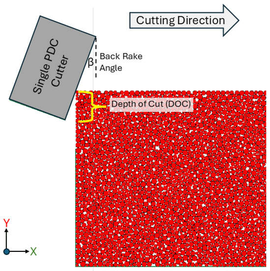
Figure 1.
PFC2D simulation at initial conditions.
At the beginning of the simulation, the cutter was placed at the leftmost corner of the SRM with a vertical offset equal to the depth of cut (DOC), which can be calculated by dividing ROP, which has units of m/min, by the number of revolutions per minute (N) as shown in the formula given below.
Cutters rotate in a 3D circular path, and this rotational motion was converted into a 2D linear motion to be modelled in PFC2D. The cutter’s linear speed (v) is calculated by the formula given below, where equals the nth cutter’s radial distance from the bit’s rotational axis.
The model was then simulated for a given time window, and Figure 2 shows a sample of fractured rock during a simulation, along with the measured forces on the cutter in the x and y directions. Axial forces generated due to rock fracture from a single cutter interaction will be equal to the y-direction forces, and torsional forces can be calculated by multiplying the x-direction force by the radial distance of the cutter from the bit rotational axis.
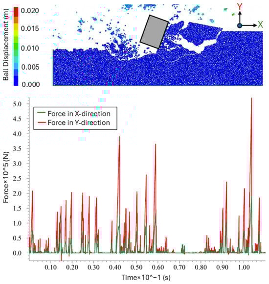
Figure 2.
Plot of PFC2D simulation output results.
To generate the dataset for model training, 240 simulations were run with different parameter settings, as shown in Table 2. Each simulation was run three times with varying seed values for ball distribution/generation, and the average of those three simulations was used to improve accuracy and account for model randomness.
Table 2.
Simulation parameters range and number of steps.
3.2. Developing an ANN Model for Rock Fracture Force Calculation
As previously mentioned, performing numerical analysis such as DEM directly in the simulation model is not feasible due to computational limitations. For example, 1 s of a single cutter PFC2D model takes around 180 min, making the simulation model unusably slow for modelling drill string dynamics. Therefore, a machine learning method trained using numerical simulation data is necessary to generate results in real time.
During the preliminary analysis, different machine learning methods were tested. Given the time-series nature of the rock fracture force data generated by PFC2D, an LSTM algorithm was initially tested for training using the test data. Due to the ability to capture long-term dependencies in sequential data, LSTM networks have been used to forecast changes in many applications, including stock prices, sales, weather and drug performances. However, initial attempts to train an LSTM algorithm on the time-series rock fracture force interaction data proved unsuccessful, primarily due to the inherent unpredictability of rock fracture force variations. Moreover, the LSTM method would require a long sequence of data, which can be time-consuming to generate using the PFC2D simulation.
Next, the ANN approach was selected due to its robust prediction ability and ease of implementation. However, ANN models are designed to be used as either a regression or classification model, which can be a challenge since this research requires the generation of time series of rock fracture force signals. Hence, a new approach was developed where the force time-series signal will be deconstructed into a set of parameters, and later, these parameters, which will be predicted by the ANN model, will be used to reconstruct the rock fracture force signal with similar characteristics. This approach is suitable because it is not necessary to create the exact force signal for each drilling condition–the objective is to capture general characteristics such as frequency distribution and amplitude.
Looking at the rock fracture force generated from the PFC2D simulation, the signal is best parameterized by the number of peaks and the distribution of those peaks. The following five parameters will be calculated
- Amplitude of the highest peak (Maximum amplitude)
- Average amplitude of all peaks
- Number of peaks in the first quadrant (75% to 100%)
- Number of peaks in the second and third quadrant (25% to 75%)
- Number of peaks in the fourth quadrant (0 to 25%)
A MATLAB (2024b) script was developed to automatically read the saved data and output the five previously mentioned parameters. The findpeaks function in MATLAB toolbox was employed to identify peaks, and a minimum peak height filter (set at >1% of maximum amplitude) was implemented to exclude insignificant peaks.
To prepare the ANN model, the generated dataset underwent preprocessing: it was scaled, randomized, and then divided into training and testing sets following an 80/20 split. Next, after evaluating several options, Keras was chosen as the development environment for the ANN model. Keras is an open-source, user-friendly, high-level API written in Python for building and training neural networks. Keras runs on top of backends like TensorFlow, PyTorch and Jax, providing an approachable, highly-productive interface that minimizes the number of actions required to preprocess, train and evaluate the ANN model [86].
Selecting an appropriate ANN architecture is vital for the model to effectively learn intricate data patterns and generate precise predictions. A suitable architecture allows the model to capture key data relationships, resulting in improved performance and better generalization. Selecting the architecture involves selecting the number of layers, nodes per layer, activation function, learning rate and evaluation criteria. These parameters were systematically selected beginning with a relatively simple model and slowly increasing the complexity until reasonable accuracy was reached without overfitting. It was decided to train five different ANN models, one for each output, instead of a single ANN model with five output nodes. This approach would produce models that are relatively simple, and easy to train/validate when compared with a single multi-output model. Furthermore, using five different ANN models will prevent negative interference from unrelated parameters and facilitate flexible training operations. All ANN models have an input layer with three nodes corresponding to the three input parameters: linear speed, depth of cut and cutter angle. After a few trials, parameters for all five ANN models were selected to have three hidden layers with 4, 6 and 3 nodes respectively, as shown in Figure 3. The activation function for all layers was selected to be Rectified Linear Unit (ReLU) because it is easy to implement and helps prevent the vanishing gradient problem. The Adams optimizer was used with the learning rate set to 0.001, and the model was evaluated using the mean squared error evaluation criteria.
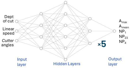
Figure 3.
Diagram of the ANN network.
The model was trained for 50 epochs with a batch size of 4, until the mean squared error on the validation dataset fell below 1%. After training, for further validation, the tuned ANN model predictions for each operational condition were compared with PFC2D results as shown in Figure 4. In this plot, the x-axis shows the PFC2D results, and the y-axis is either the ANN predictions or the PFC2D results. These results show that the maximum ANN deviation from the identity line was less than 15% and the average deviation was less than 1%, which would be sufficient for this application. Furthermore, considering the randomness of the bit-rock interaction, exact prediction is difficult and unnecessary.
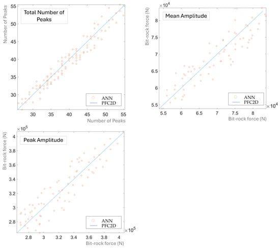
Figure 4.
Validation of the trained ANN network.
3.3. Generating the Rock Fracture Force Time Series Signal from ANN Results
The objective of this subsection is to recreate the bit-rock force time series, and represent a complete PDC bit using superposition of multiple single-cutter ANN model outputs.
As the first step, a single cutter ANN model was developed as shown in Figure 5. The left side of the figure shows the four inputs, and the right side shows the output forces from the rock fracture model. “ROP to DepthCut” and “RPM to Linear Speed” are two submodels that convert the MBD parameters into the required inputs for the ANN model. The “F2T” submodel converts the rock fracture forces in the x direction predicted by the ANN model into torques by multiplying the radial distance () of the cutter from the rotational axis for the complete PDC bit.
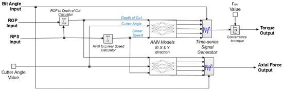
Figure 5.
Single cutter bit-rock interaction submodel.
The ANN block shown in the figure contains all the weights and biases of the tuned ANN models and has matrix operations to generate the ANN outputs for a given input value. The number of peaks (, and ) from the ANN model was divided by RPS and , so that the values represent the number of peaks for a given angle of rotation () based on the PFC2D simulation window. Without these scaling operations, the number of peaks that would be predicted by the model would depend on different rotational angles due to the difference in linear speed in the PFC2D simulation.
The ANN post-processing algorithm was written using simple functions such as for loops and if conditions so that it can be implemented in the MBD development environment without requiring resource-intensive co-simulation methods.
In this approach, arrays were created for the amplitude of each peak () and the bit rotational angle () at which each peak will occur. The array has elements equal to the total number of peaks predicted by the ANN model, and the values for each of these were filled using random numbers that are generated between zero and the . Given below is the syntax for this implementation, and indicates the random number function.
| for i = 1 to () |
| end |
Filling of the array was done in two steps. The first step has three for loops corresponding to the three outputs (, and ) from the ANN model. All these were looped one after the other, filling elements equal to each number of peaks using a random value and the syntax for these for loops is given below.
| for j = 1 to |
| A[j] = (0.75∗) + (0.25∗∗) |
| end |
| for k = 1 to |
| A[ + k] = (0.25∗) + (0.50∗∗) |
| end |
| for l = 1 to |
| A[ + + l] = (0.25∗∗) |
| end |
In the second step, these peaks were modified so that the maximum and peak information would be accurate. To include the maximum peak, the first element in the was modified to be equal to . To match the mean value, all remaining array elements were multiplied by a scaling factor (), which is equal to;
The next step would be to recreate the shape of each peak. This was achieved by using the STEP5 function, which is a mathematical function used to create a smooth transition between two values and the equation for this function is given below,
where
- x = the independent variable
- = the x value at which the STEP5 function begins
- = the value of the STEP5 function desired at
- = the x value at which the STEP5 function ends
- = the value of the STEP5 function desired at
To recreate the shape of each peak, two STEP5 functions were combined to generate the rising and falling sides of the curve. The independent variable for this application will be the remainder of the bit rotational angle () after dividing by the angle. Hence, the independent variable will repeat as the bit rotates, resetting as it passes the angle window, in which the ANN outputs are given. For each simulation time step, there will be a for loop that goes through all array elements in the angle and amplitude array and will create an output based on the independent variable, two arrays and the STEP5 function.
Up to now, all the calculations and DEM simulations were performed for a single cutter element. A full PDC bit has multiple of these single cutters placed at various radial distances from the rotational axis of the bit. To recreate the full bit-rock excitation forces of a PDC bit, multiple single-cutter submodels with different based on the location of each cutter have to be combined together as shown in Figure 6. In this approach, the bit-rock forces from the full PDC bit are assumed to be the summation of the bit force generated by each cutter. The random number generators in each of these elements will have different seed values so that the force peaks from each cutter are randomly distributed. This figure also shows the implementation of a moving average function. The objective of this operation is to smooth out variations in ROP and RPS that are given by the MBD model outputs. The moving average function takes the average variation for a 0.1-s time window. This removes the high-frequency changes in ROP and RPS, which would not be useful for calculating bit-rock forces and can cause instabilities in the ANN model.
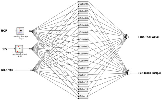
Figure 6.
Complete bit rock interaction model.
3.4. Developing a Drill String MBD Simulation Model with Bit-Rock Interaction
A rigid segment model of the drill string was developed to test and implement the model. This simple model has two axial rigid masses and two torsional rigid masses that are connected in series with parallel spring-damper elements as shown in Figure 7.
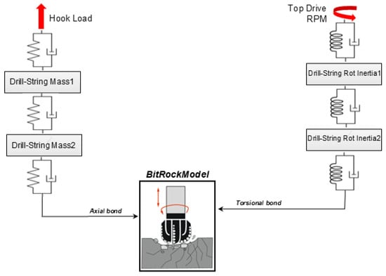
Figure 7.
Drill string MBD model with bit rock interaction model.
The total mass and rotational inertia of the drill string were divided between the two lumped segments, and the coefficients for the spring values were calculated based on the equations given in [87].
In the above equations, E and G are the elastic modulus, I is the area moment, j is the polar moment of area, A is the cross-sectional area, and is the segment length. The drill string mass submodel also provides the gravitational force, which helps to generate the WOB. The coupling of axial and torsional drill string segments will happen through the bit-rock interaction submodel, and it will be discussed in the following subsection.
3.5. Bit-Rock Interaction Submodel
The bit-rock interaction model has several components to accurately model the interactions between the bit and the rock substrate. These can be divided into the following subsections.
- Inertia components of the bit
- Axial hydraulic force due to drilling mud jets at the bit
- Bit rotation angle calculation
- Frictional force due to bit-rock contact
- Rock fracture ANN model
- Axial vibrations generated due to rock fracture
- Torsional vibrations generated due to rock fracture
- Stiffness and damping of the rock substrate
- Drilling progression and bit advancement
The mass of the bit and rotational inertia were included as axial and torsional components, and the gravitational force was also applied in the axial direction. Bit hydraulic force () due to drilling mud jets was calculated using the formula given below, where is the pressure ROP at the bit and is the total area of bit hydraulic nozzle orifices.
The bit can sometimes rotate during a drilling operation without causing rock penetration, due to insufficient WOB. Moreover, during stick-slip conditions, the bit can rotate in the negative direction. The bit rotation calculation submodel calculates the bit progression angle (), which indicates the angle that the bit has rotated in the positive direction while the weight on bit (WOB) is above a given threshold value. Figure 8 shows the steps for calculating the bit progression angle, where is the bit rotational velocity, and indicates the threshold WOB value.

Figure 8.
Bit rotation calculation steps.
As the name implies, the ROP submodel calculates the ROP for given simulation operation conditions. This submodel calculates ROP based on the modified ROP equation from [88]. In this equation, , and depend on the bit type and formation.
In addition to the cutting torque applied from the rock fracture ANN model, there is also frictional TOB, and this was calculated [88] using the frictional equations given below. In that equation is a function that characterizes the frictional process, and , , , , and are experimentally-determined parameters.
The development of the rock fracture ANN submodel was explained in Section 3.3, and that model has two rock fracture component outputs: axial force and rotational torque. Implementation of the torsional is via a special spring element where the spring stiffness coefficient () depends on the instantaneous torsion-creating force output value from the bit-rock interaction model. This spring element does not carry tensile forces and has zero stiffness when the bit is rotating in the negative direction. This enables the emulation of the rock’s resistance to fracture and the rock’s compliance in a torsional direction. The implementation of axial rock fracture force is comparatively straightforward when compared with the rotational torque component; for the given value, the ANN model will generate an axial rock fracture force, which is applied to the bit as shown in Figure 9.
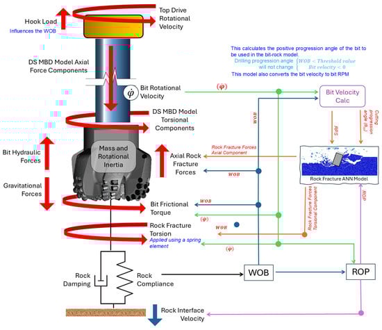
Figure 9.
Bit-rock interaction sub model.
The final component of the bit-rock submodel is the modelling of drilling progression based on the ROP value. This is achieved by modelling and moving a virtual rock interface based on the ROP prediction. The compliance of the rock is modelled by placing an axial spring/damper between the bit and the rock interface. This rock compliance axial spring has a high compressive and zero tensile stiffness. Therefore, during off-bottom and bit-bounce conditions, the force from this spring element will be zero. The force from this spring element is equal to the reaction force on the bit by the rock substrate. Since the reaction force is equal to WOB, this spring element was also utilized to provide the WOB signal value to be used by other components. To model drill bit progression, axial velocity equal to the predicted ROP was applied to the rock interface.
Combining all these submodels enables the emulation of realistic behaviour between rock and bit, including bit-rock interaction, frictional force, inertia forces, and bit hydraulic forces. These models enable prediction of WOB, TOB and ROP and provide excitational force and boundary conditions for the simulation model. The results from this model will be given in Section 4.1, where a case study of stick-slip and bit-bounce conditions will be analyzed.
3.6. Implementing the Bit-Rock Model in a 3D Deviated Well Drill String MBD Model
The previous subsection provided a description of a simple 2D drill string model limited to vertical wells, without wellbore contact. Deviated well drillstring response can be simulated utilizing a 3D MBD simulation model developed by the authors of this paper and published in [89].
The model uses 3D rigid segment elements based on the Newton-Euler formulation and has axial, torsional, lateral and bending springs between those elements to include drill string flexibility. A friction-based contact model was also implemented in the model to account for interactions between the drill string and the well bore, which will influence whirling and lateral vibrational behaviour. This contact model detection algorithm is applicable to all parts of the wellbore, including vertical, horizontal, and build sections, and does not require special elements/methods for each section. Readers should refer to [89] for more details about the contact algorithm and [90] for the development of the rigid segment drill string dynamics model. This simulation model can emulate drilling progression and tripping by using a special variable-length top segment and velocity constraint at the bit to guide it along the well profile.
Implementing the bit-rock submodel in the 3D MBD model will be similar to that of the 2D simulation model. The 2D model only had axial and torsional components, compared to the six degrees of freedom (three translational and three rotational) of the 3D MBD model. However, when considering bit-rock force, axial and bit rotation are the only important components. Therefore, only those components were modified when implementing the bit-rock submodel in the 3D MBD model. Section 4.2 provides a case study incorporating the bit-rock force prediction method into the 3D drill string model.
4. Case Studies
The following case studies show the functionality of the bit-rock interaction model and its ability to provide excitation forces for MBD simulations, which helps to predict rich stress history information, enabling improved fatigue prognosis. The first case study utilizes a 2D drill string MBD model to show different bit vibration conditions, and the second case study utilizes a 3D MBD model to show the effects of the bit-rock interaction model on the stress predictions for a downhole component in a deviated well.
4.1. 2D Drill String Model Under Severe Vibrations
The 2D MBD model developed in Section 3.4 was used to show the flexibility of the bit rock interaction model to predict bit vibrations under different conditions, including stick-slip, bit-bounce, and normal operational conditions. The total length of the drill string was 150 m. For the top boundary condition axial force was applied to create the hook load, and rotational velocity was applied to represent the top drive motor. The bottom boundary condition was applied using the bit-rock interaction model, which provides the coupling between axial and torsional segments.
Figure 10 shows the simulation of normal operational conditions. The top drive rotational speed was set at 60 rpm, and the hook load was 25 kN. In this model, a variation in WOB, ROP and bit rotational speed was observed due to the changes in the bit excitation.
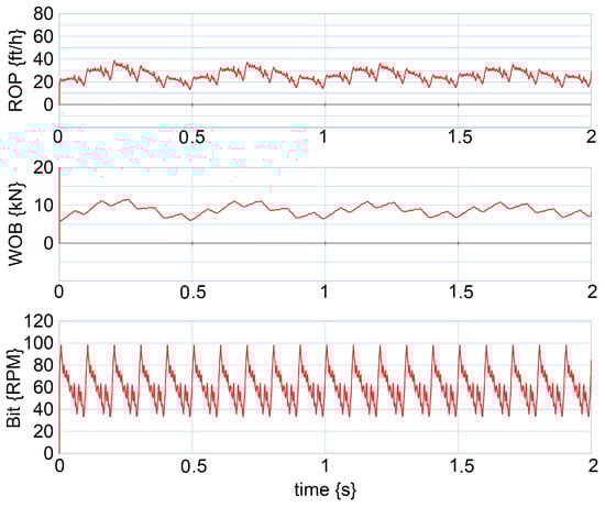
Figure 10.
Normal operational conditions simulation results from the 2D MBD model.
Significantly increasing WOB and reducing drilling RPM will eventually induce stick-slip behaviour. To test the model’s ability to capture this, the hook load was reduced to 15 kN, and the top drive speed was set to 30 rpm. The result from this simulation is given in Figure 11, which shows that the drill bit rotational speed becomes zero or even rotates in the negative direction for a few milliseconds, and then speeds back up above the top drive rotational rpm.
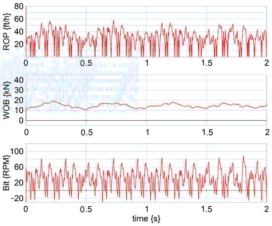
Figure 11.
Stick-slip condition simulation results from the 2D MBD model.
Another common drilling problem, bit bounce, can be induced by lowering static WOB through increased hook load. Figure 12 shows bit bounce condition simulation results and the variations in dynamic WOB when the hook load was increased to 35.5 kN.
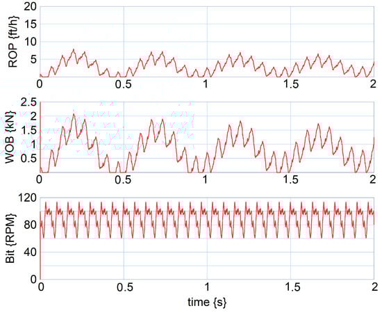
Figure 12.
Bit-bounce condition simulation results from the 2D MBD model.
From these case studies, it can be observed that the bit-rock model is capable of recreating typical drilling problems, while providing additional excitation components to the drill string that would be absent with overly simple sinusoidal or white noise approaches.
4.2. 3D Deviated Well Drill String MBD Simulation with Bit-Rock Interaction Model
The objective of the case study is to show the utilization of the bit-rock model in a deviated well 3D MBD simulation model, and contrast the ANN-generated bit-rock excitation with sinusoidal excitation. The parameters of the sinusoidal excitation force were selected to match the bit-rock excitation forces for easy comparison. Both models have 100 drill pipe segments and 20 drill collar segments. The dimensions and material properties of rigid segments are given in the Table 3 below.
Table 3.
Drill pipe and collar simulation parameters.
This 3D drill string simulation model utilizes a deviated well profile as shown in Figure 13 and has a non-linear contact/friction model between the drill string and the wellbore. The deviated well profile has a high dog-leg severity (10 degrees per 30 m) curve until reaching horizontal
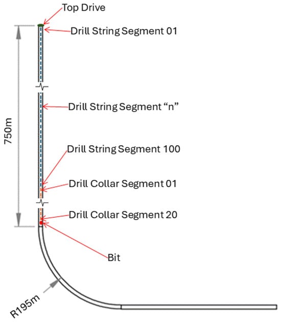
Figure 13.
Well profile for 3D deviated well case study.
This model begins simulation with all drill string segments in the vertical section and the bit at the end of the vertical section. The first drill segment of this simulation model is a special element that is designed to increase its length as drilling/tripping progresses. The simulation operation has two parts; for the first 300 s, the drill pipe is tripped in at a speed of 1.00 m/s. Afterwards, the model simulates the drilling operation for a given ROP value of 0.005 m/s (60 ft/hr) and drill string rotational speed of 60 rpm provided by the top drive.
Figure 14 shows the stress history information for several points in the drill string during the drilling operation, starting at 325 s for a 25-s time window. Since the model begins with the bit near the end of the vertical section and trips 300 m during the first 300 s of the simulation, the bit has completed the build section and progressed 25 m into the horizontal section.
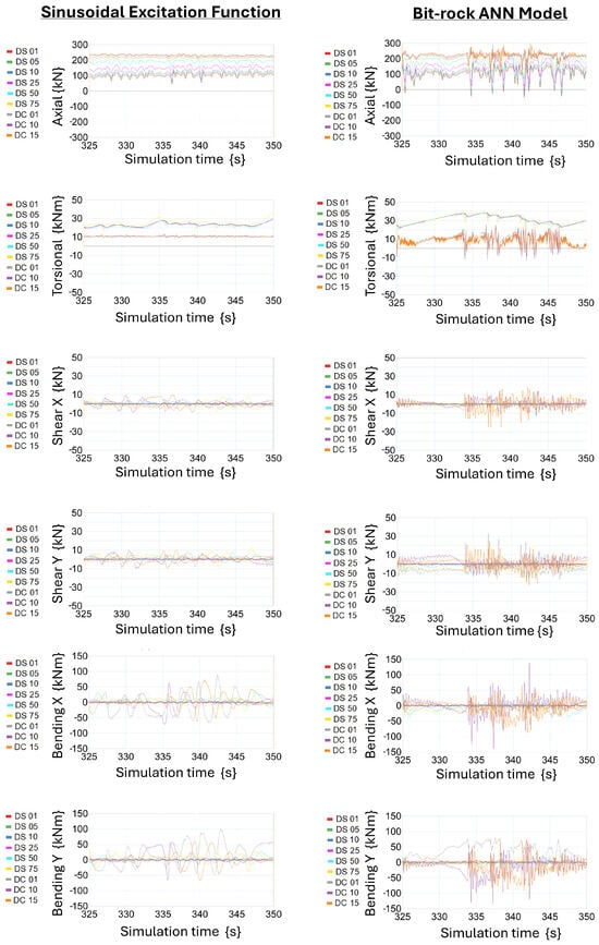
Figure 14.
Stress history comparison between ANN bit-rock model vs. sinusoidal.
These results show major differences in stress history between sinusoidal excitation functions and the ANN bit-rock model. High-frequency force components present with the new bit-rock model are not present in the sinusoidal excitation model. This shows that after validation, the bit-rock model will facilitate the generation of more realistic stress history information for downhole components.
5. Conclusions and Future Work
Drilling simulation models have been utilized in modern industrial applications to improve performance and predict the durability of downhole equipment. Most current simulation models use simplified approaches, such as cosine or random functions, to model bit-rock interaction, leading to overly simplistic excitation forces that impede model prediction accuracy.
Due to the complexity of the rock fractures, developing such a model based on theoretical equations or first principles is challenging. Hence, this research aimed to create a fast, user-friendly alternative.
This objective was achieved successfully by developing an ANN model trained using bit-rock force variations generated by a DEM simulation model. Bit inertia, friction, and hydraulic forces were also included to create a comprehensive bit submodel that can be implemented in existing MBD simulations. After comparing both 2D and 3D approaches, the 2D single-cutter DEM simulation model was selected for this research due to its faster simulation time. After generating the dataset, the ANN model was trained using the Keras open-source deep learning platform. Next, an algorithm was developed to recreate the bit-rock force time series.
A 2D MBD model was used to test the bit-rock model and perform analysis for severe bit vibration conditions such as stick-slip and bit-bounce. Afterwards, the bit rock model was implemented in a 3D deviated well drill string model with contact and non-linear friction to create a comprehensive simulation model capable of modelling different drilling conditions. This model provided rich stress history information, which would benefit future simulation-based design exercises.
The DEM rock model used in this research has been validated against UCS experimental data. However, the force variation and fracture profiles during drilling have yet to be tested and validated. Hence, one of the future aims is to validate the bit-rock model. Another future goal is to utilize a fully three-dimensional DEM bit model, which would enable modelling the effects of prefractured rock and interaction between cutters. A complete PDC bit model would also facilitate the calculation of bit lateral forces missing in the current method.
The bit-rock model was trained for a single rock material type and only applies to PDC bits. In the future, the model’s applicability can be expanded by training it on various rock types and adapting it to different bit types, such as roller cone bits. This may require developing a new DEM model to simulate the crushing action of roller cone teeth rather than the shearing action of PDC cutters. When modelling roller cone bits, it might be beneficial to superimpose a sinusoidal function in addition to the ANN bit-rock model to emulate the uneven multilobe rock surfaces, which can sometimes be generated due to the tri-cone design of the bit.
The current ANN approach does not model the periods of zero bit-rock force that occur when rock fragments are removed, even though the DEM simulation has captured this behaviour. This limitation can be rectified by refining the ANN input to include information about the number of force peaks against angle/time quadrants, in addition to the current amplitude quadrants. This will allow the distribution of zero-force periods due to the rock fragment removal to be included in the dynamic simulation.
In summary, this research trained an ANN model using simulation data to predict bit-rock forces, and utilized the model in a MBD simulation. This modelling approach has the potential to be applied in other fields where predicting complex excitation forces from first principles is a challenge.
Author Contributions
S.L.: Conceptualization, methodology, analysis, original draft preparation. G.R.: review and editing, supervision, project administration, funding acquisition. All authors have read and agreed to the published version of the manuscript.
Funding
This research was funded by Natural Science and Engineering Research Council of Canada (NSERC) [Funding reference number 03887-2018].
Data Availability Statement
The data that support the findings of this study are available on request from the corresponding author.
Conflicts of Interest
The authors declare no conflicts of interest.
Abbreviations
The following abbreviations are used in this manuscript:
| ANFIS | adaptive neuro-fuzzy inference system |
| AI | artifical inteligence |
| ANN | artificial neutral networks |
| BEM | boundary element method |
| BPM | bonded-particle model |
| DEM | discrete element method |
| DFN | discrete fracture networks |
| DOC | depth of cut |
| DT | decision trees |
| FDM | finite difference method |
| FEA | finite element analysis |
| FEM | finite element method |
| FN | functional network |
| HMM | hidden Markov models |
| KNN | K-nearest neighbour |
| PDC | Polycrystalline Diamond Compact |
| PFC | Particle Flow Code |
| LSTM | Long Short-Term Memory |
| ML | machine learning |
| MBD | multibody dynamics |
| NPT | non-productive time |
| RBF | radial basis function |
| ReLU | Rectified Linear Unit |
| ROP | rate of penetration |
| RPM | revolutions per minute |
| RNN | Recurrent neural networks |
| SVM | support vector machines |
| SRM | synthetic rock material |
| UCS | unconfined compressive strength |
| WOB | weight on bit |
References
- Li, M.; Liu, J.; Xia, Y. Risk prediction of gas hydrate formation in the wellbore and subsea gathering system of deep-water turbidite reservoirs: Case analysis from the south China Sea. Reserv. Sci. 2025, 1, 52–72. [Google Scholar] [CrossRef]
- Vanja. How Much Does a Drilling Rig Cost?—SOSS USA. Available online: https://sossusa.com/2024/09/16/how-much-does-a-drilling-rig-cost (accessed on 15 December 2025).
- Li, Q.; Liu, J.; Wang, S.; Guo, Y.; Han, X.; Li, Q.; Cheng, Y.; Dong, Z.; Li, X.; Zhang, X. Numerical insights into factors affecting collapse behavior of horizontal wellbore in clayey silt hydrate-bearing sediments and the accompanying control strategy. Ocean. Eng. 2024, 297, 117029. [Google Scholar] [CrossRef]
- Li, Q.; Li, Q.; Han, Y. A numerical investigation on kick control with the displacement kill method during a well test in a deep-water gas reservoir: A case study. Processes 2024, 12, 2090. [Google Scholar] [CrossRef]
- Jaime, M.C. Numerical Modeling of Rock Cutting and Its Associated Fragmentation Process Using the Finite Element Method. Ph.D. Thesis, University of Pittsburgh, Pittsburgh, PA, USA, 2011. [Google Scholar]
- Cai, M.; Mao, D.; Li, X.; Peng, H.; Tan, L.; Gui, Y.; Yin, X. Downhole vibration characteristics of 3D curved well under drillstring–bit–rock interaction. Int. J. -Non-Linear Mech. 2023, 154, 104430. [Google Scholar] [CrossRef]
- Richard, T.; Germay, C.; Detournay, E. A simplified model to explore the root cause of stick–slip vibrations in drilling systems with drag bits. J. Sound Vib. 2007, 305, 432–456. [Google Scholar] [CrossRef]
- Aarsnes, U.J.F.; Shor, R.J. Torsional vibrations with bit off bottom: Modeling, characterization and field data validation. J. Pet. Sci. Eng. 2018, 163, 712–721. [Google Scholar] [CrossRef]
- Saldivar, B.; Mondié, S.; Niculescu, S.I.; Mounier, H.; Boussaada, I. A control oriented guided tour in oilwell drilling vibration modeling. Annu. Rev. Control 2016, 42, 100–113. [Google Scholar] [CrossRef]
- Wei, J.; Liu, W.; Gao, D. Modeling of PDC bit-rock interaction behaviors based on the analysis of dynamic rock-cutting process. Geoenergy Sci. Eng. 2024, 239, 212955. [Google Scholar] [CrossRef]
- Mao, L.; He, J.; Zhu, J.; Jia, H.; Gan, L. Dynamic characteristic response of PDC bit vibration coupled with drill string dynamics. Geoenergy Sci. Eng. 2024, 233, 212524. [Google Scholar] [CrossRef]
- Kreisle, L.F.; Vance, J.M. Mathematical analysis of the effect of a shock sub on the longitudinal vibrations of an oilwell drill string. Soc. Pet. Eng. J. 1970, 10, 349–356. [Google Scholar] [CrossRef]
- Macpherson, J.; Jogi, P.; Kingman, J. Application and analysis of simultaneous near bit and surface dynamics measurements. SPE Drill. Complet. 2001, 16, 230–238. [Google Scholar] [CrossRef]
- Dareing, D.; Livesay, B.J. Longitudinal and angular drill-string vibrations with damping. J. Eng. Ind. 1968, 90, 671–679. [Google Scholar] [CrossRef]
- Christoforou, A.; Yigit, A. Dynamic modelling of rotating drillstrings with borehole interactions. J. Sound Vib. 1997, 206, 243–260. [Google Scholar] [CrossRef]
- Sarker, M.; Rideout, D.G.; Butt, S.D. Dynamic model for 3D motions of a horizontal oilwell BHA with wellbore stick-slip whirl interaction. J. Pet. Sci. Eng. 2017, 157, 482–506. [Google Scholar] [CrossRef]
- Jansen, J.D.; Van Den Steen, L. Active damping of self-excited torsional vibrations in oil well drillstrings. J. Sound Vib. 1995, 179, 647–668. [Google Scholar] [CrossRef]
- Kanzari, M. Effects of Drill Mud and Drive Torque Sinusoidal Excitation on Drillstrings Lateral and Torsional StickSlip Vibrations. In Proceedings of the Qatar Foundation Annual Research Conference Proceedings, Doha, Qatar, 19–20 March 2018; HBKU Press: Doha, Qatar, 2018; Volume 2018, p. EEPD868. [Google Scholar]
- Qiu, H.; Yang, J.; Butt, S. Stick-Slip Analysis of a Drill String Subjected to Deterministic Excitation and Stochastic Excitation. Shock Vib. 2016, 2016, 9168747. [Google Scholar] [CrossRef]
- Skaugen, E. The effects of quasi-random drill bit vibrations upon drillstring dynamic behavior. In Proceedings of the SPE Annual Technical Conference and Exhibition? Dallas, TX, USA, 27–30 September 1987; SPE: Richardson, TX, USA, 1987. [Google Scholar]
- Spanos, P.; Chevallier, A.; Politis, N. Nonlinear stochastic drill-string vibrations. J. Vib. Acoust. 2002, 124, 512–518. [Google Scholar] [CrossRef]
- Ritto, T. Numerical Analysis of the Nonlinear Dynamics of a Drill-String with Uncertainty Modeling. Ph.D. Thesis, Université Paris-Est, Paris, France, Pontifícia Universidade Católica, Rio de Janeiro, Brésil, 2010. [Google Scholar]
- Bogdanoff, J.; Goldberg, J. A new analytical approach to drill pipe breakage II. J. Eng. Ind. 1961, 83, 101–106. [Google Scholar] [CrossRef]
- Qiu, H.; Yang, J.; Butt, S.; Zhong, J. Investigation on random vibration of a drillstring. J. Sound Vib. 2017, 406, 74–88. [Google Scholar] [CrossRef]
- He, J.; Li, Y.; Jin, Y.; Wang, A.; Zhang, Y.; Jia, J.; Song, H.; Liang, D. Study on mechanical problems of complex rock mass by composite material micromechanics methods: A literature review. Front. Earth Sci. 2022, 9, 808161. [Google Scholar] [CrossRef]
- Potyondy, D.O.; Cundall, P.A. A bonded-particle model for rock. Int. J. Rock Mech. Min. Sci. 2004, 41, 1329–1364. [Google Scholar] [CrossRef]
- Starfield, A.M.; Cundall, P. Towards a methodology for rock mechanics modelling. In Proceedings of the International Journal of Rock Mechanics and Mining Sciences & Geomechanics Abstracts; Elsevier: Amsterdam, The Netherlands, 1988; Volume 25, pp. 99–106. [Google Scholar]
- Agharazi, A. Development of a 3D Equivalent Continuum Model for Deformation Analysis of Systematically Jointed Rock Masses; University of Alberta: Edmonton, AB, Canada, 2013. [Google Scholar]
- Lisjak, A.; Grasselli, G. A review of discrete modeling techniques for fracturing processes in discontinuous rock masses. J. Rock Mech. Geotech. Eng. 2014, 6, 301–314. [Google Scholar] [CrossRef]
- Tezuka, A. Finite element and finite difference methods. In Springer Handbook of Metrology and Testing; Springer: Berlin/Heidelberg, Germany, 2011; pp. 1033–1060. [Google Scholar]
- Fang, Z. A Local Degradation Approach to the Numerical Analysis of Brittle Fractures in Heterogeneous Rocks. Ph.D. Thesis, Imperial College London (University of London), London, UK, 2001. [Google Scholar]
- Jing, L.; Hudson, J. Numerical methods in rock mechanics. Int. J. Rock Mech. Min. Sci. 2002, 39, 409–427. [Google Scholar] [CrossRef]
- Logan, D.L. A First Course in the Finite Element Method; Cengage Learning: Boston, MA, USA, 2011; Volume 4. [Google Scholar]
- Chiang, L.E.; Elias, D.A. A 3D FEM methodology for simulating the impact in rock-drilling hammers. Int. J. Rock Mech. Min. Sci. 2008, 45, 701–711. [Google Scholar] [CrossRef]
- Hammah, R.; Yacoub, T.; Corkum, B.; Curran, J. The practical modelling of discontinuous rock masses with finite element analysis. In Proceedings of the ARMA US Rock Mechanics/Geomechanics Symposium, San Francisco, CA, USA, 1–4 June 2008; ARMA: Arlington, VA, USA, 2012. [Google Scholar]
- Wang, J.K.; Lehnhoff, T. Bit penetration into rock—A finite element study. In Proceedings of the International Journal of Rock Mechanics and Mining Sciences & Geomechanics Abstracts; Elsevier: Amsterdam, The Netherlands, 1976; Volume 13, pp. 11–16. [Google Scholar]
- Harewood, F.; McHugh, P. Comparison of the implicit and explicit finite element methods using crystal plasticity. Comput. Mater. Sci. 2007, 39, 481–494. [Google Scholar] [CrossRef]
- Goodman, R.E.; Taylor, R.L.; Brekke, T.L. A model for the mechanics of jointed rock. J. Soil Mech. Found. Div. 1968, 94, 637–659. [Google Scholar] [CrossRef]
- Beissel, S.; Johnson, G.; Popelar, C. An element-failure algorithm for dynamic crack propagation in general directions. Eng. Fract. Mech. 1998, 61, 407–425. [Google Scholar] [CrossRef]
- Rabczuk, T. Computational methods for fracture in brittle and quasi-brittle solids: State-of-the-art review and future perspectives. Int. Sch. Res. Not. 2013, 2013, 849231. [Google Scholar] [CrossRef]
- Jaime, M.C.; Zhou, Y.; Lin, J.S.; Gamwo, I.K. Finite element modeling of rock cutting and its fragmentation process. Int. J. Rock Mech. Min. Sci. 2015, 80, 137–146. [Google Scholar] [CrossRef]
- Paluszny, A.; Salimzadeh, S.; Zimmerman, R.W. Finite-element modeling of the growth and interaction of hydraulic fractures in poroelastic rock formations. In Hydraulic Fracture Modeling; Elsevier: Amsterdam, The Netherlands, 2018; pp. 1–19. [Google Scholar]
- Lu, Z.; Wan, L.; Zeng, Q.; Zhang, X.; Gao, K. Numerical simulation of fragment separation during rock cutting using a 3D dynamic finite element analysis code. Adv. Mater. Sci. Eng. 2017, 2017, 3024918. [Google Scholar] [CrossRef]
- Li, G.; Wang, K.; Tang, C.; Ye, J. Non-break modeling and numerical simulation for non-intact rock failure process. Int. J. Rock Mech. Min. Sci. 2024, 176, 105725. [Google Scholar] [CrossRef]
- Costabel, M. Principles of boundary element methods. Comput. Phys. Rep. 1987, 6, 243–274. [Google Scholar] [CrossRef]
- Blandford, G.E.; Ingraffea, A.R.; Liggett, J.A. Two-dimensional stress intensity factor computations using the boundary element method. Int. J. Numer. Methods Eng. 1981, 17, 387–404. [Google Scholar] [CrossRef]
- Chen, C.S.; Pan, E.; Amadei, B. Fracture mechanics analysis of cracked discs of anisotropic rock using the boundary element method. Int. J. Rock Mech. Min. Sci. 1998, 35, 195–218. [Google Scholar] [CrossRef]
- Zeller, S.S.; Pollard, D.D. Boundary conditions for rock fracture analysis using the boundary element method. J. Geophys. Res. Solid Earth 1992, 97, 1991–1997. [Google Scholar] [CrossRef]
- Mi, Y.; Aliabadi, M. Dual boundary element method for three-dimensional fracture mechanics analysis. Eng. Anal. Bound. Elem. 1992, 10, 161–171. [Google Scholar] [CrossRef]
- Cundall, P.A. A computer model for simulating progressive, large-scale movement in blocky rock system. In Proceedings of the International Symposium on Rock Mechanics, Nancy, France, 4–6 October 1971; Volume 8, pp. 129–136. [Google Scholar]
- Joodi, B. Application of 3D Discrete Element Method in Geomechanics, with A Focus on Rock Scratch Testing. Ph.D. Thesis, Curtin University, Bentley, Australia, 2018. [Google Scholar]
- Potyondy, D.O. The bonded-particle model as a tool for rock mechanics research and application: Current trends and future directions. Geosystem Eng. 2015, 18, 1–28. [Google Scholar] [CrossRef]
- Potyondy, D. A flat-jointed bonded-particle model for rock. In Proceedings of the ARMA US Rock Mechanics/Geomechanics Symposium, Seattle, DC, USA, 17–20 June 2018. [Google Scholar]
- Tsang, M.; Clark, I.; Karlovšek, J. Automating the Calibration of Flat-Jointed Bonded Particle Model Microproperties for the Rewan Sandstone Case Study. Rock Mech. Rock Eng. 2023, 56, 6459–6480. [Google Scholar] [CrossRef]
- Huang, H. Discrete Element Modeling of Tool-Rock Interaction; University of Minnesota: Minneapolis, MN, USA, 1999. [Google Scholar]
- Yaşıtlı, N.E.; Bayram, F.; Unver, B.; Özçelik, Y. Numerical modelling of circular sawing system using discrete element method. Int. J. Rock Mech. Min. Sci. 2012, 55, 86–96. [Google Scholar] [CrossRef]
- Zhang, H.; Ni, H.; Yang, H.; Fu, L.; Wang, Y.; Liu, S.; Huang, B.; Wang, Z.; Chen, G. Numerical simulation and field test research on vibration reduction of PDC cutting of pebbled sandstone under composite impact load. Processes 2023, 11, 671. [Google Scholar] [CrossRef]
- Zheng, Z.; Tang, H.; Zhang, Q.; Pan, P.; Zhang, X.; Mei, G.; Liu, Z.; Wang, W. True triaxial test and PFC3D-GBM simulation study on mechanical properties and fracture evolution mechanisms of rock under high stresses. Comput. Geotech. 2023, 154, 105136. [Google Scholar] [CrossRef]
- Li, P.; Jiang, S.; Tang, D.; Xu, B. A PFC3D-based numerical simulation of cutting load for lunar rock simulant and experimental validation. Adv. Space Res. 2017, 59, 2583–2599. [Google Scholar] [CrossRef]
- Pierce, M.; Fairhurst, C. Synthetic rock mass applications in mass mining. In Proceedings of the ISRM Congress, Beijing, China, 18–21 October 2011; 12th ISRM Congress: Lisboa, Portugal, 2011. [Google Scholar]
- Chen, Y.; Rao, J.; Zhao, C.; Xue, Y.; Liu, C.; Yin, Q. Strength prediction model of fractured dolomite and analysis of mechanical properties based on PFC3D. Sci. Rep. 2023, 13, 13368. [Google Scholar] [CrossRef]
- Samuel, A.L. Some studies in machine learning using the game of checkers. IBM J. Res. Dev. 1959, 3, 210–229. [Google Scholar] [CrossRef]
- Morales, E.F.; Escalante, H.J. A brief introduction to supervised, unsupervised, and reinforcement learning. In Biosignal Processing and Classification Using Computational Learning and Intelligence; Elsevier: Amsterdam, The Netherlands, 2022; pp. 111–129. [Google Scholar]
- Nasteski, V. An overview of the supervised machine learning methods. Horizons. b 2017, 4, 56. [Google Scholar] [CrossRef]
- Patel, A.A. Hands-on Unsupervised Learning Using Python: How to Build Applied Machine Learning Solutions from Unlabeled Data; O’Reilly Media: Sebastopol, CA, USA, 2019. [Google Scholar]
- Li, Y. Deep reinforcement learning: An overview. arXiv 2017, arXiv:1701.07274. [Google Scholar]
- Mohanraj, T.; Yerchuru, J.; Krishnan, H.; Aravind, R.N.; Yameni, R. Development of tool condition monitoring system in end milling process using wavelet features and Hoelder’s exponent with machine learning algorithms. Measurement 2021, 173, 108671. [Google Scholar] [CrossRef]
- Manasa, J.; Gupta, R.; Narahari, N. Machine learning based predicting house prices using regression techniques. In Proceedings of the 2020 2nd International conference on innovative mechanisms for industry applications (ICIMIA), Bangalore, India, 5–7 March 2020; IEEE: New York, NY, USA, 2020; pp. 624–630. [Google Scholar]
- Vidyullatha, P.; Rao, D.R. Machine learning techniques on multidimensional curve fitting data based on R-square and chi-square methods. Int. J. Electr. Comput. Eng. 2016, 6, 974. [Google Scholar]
- Barillaro, L. Artificial Neural Networks. In Encyclopedia of Bioinformatics and Computational Biology, 2nd ed.; Ranganathan, S., Cannataro, M., Khan, A.M., Eds.; Elsevier: Oxford, UK, 2025; pp. 141–145. [Google Scholar] [CrossRef]
- Szandała, T. Review and comparison of commonly used activation functions for deep neural networks. In Bio-Inspired Neurocomputing; Springer: Berlin/Heidelberg, Germany, 2020; pp. 203–224. [Google Scholar]
- Alnuaimi, A.F.; Albaldawi, T.H. An overview of machine learning classification techniques. In Proceedings of the BIO Web of Conferences, Copenhagen, Denmark, 25–30 August 2024; EDP Sciences: Les Ulis Cedex A, France, 2024; Volume 97, p. 00133. [Google Scholar]
- Saadeldin, R.; Gamal, H.; Elkatatny, S.; Abdulraheem, A. Intelligent model for predicting downhole vibrations using surface drilling data during horizontal drilling. J. Energy Resour. Technol. 2022, 144, 083002. [Google Scholar] [CrossRef]
- Saadeldin, R.; Gamal, H.; Elkatatny, S. Detecting downhole vibrations through drilling horizontal sections: Machine learning study. Sci. Rep. 2023, 13, 6204. [Google Scholar] [CrossRef] [PubMed]
- Okoli, P.; Cruz Vega, J.; Shor, R. Estimating downhole vibration via machine learning techniques using only surface drilling parameters. In Proceedings of the SPE Western Regional Meeting, San Jose, CA, USA, 23–26 April 2019; SPE: Richardson, TX, USA. [Google Scholar]
- Don, M.G.; Rideout, G. A digital twinning methodology for vibration prediction and fatigue life prognosis of vertical oil well Drillstrings. IEEE Access 2023, 11, 62892–62905. [Google Scholar] [CrossRef]
- Wang, X.; Wang, X.; Lu, J.; Li, W.; Xue, Q.; Zhang, C.; Zhang, F. Automated classification of drill string vibrations using machine learning algorithms. Geoenergy Sci. Eng. 2024, 239, 212995. [Google Scholar] [CrossRef]
- Brenjkar, E.; Delijani, E.B. Computational prediction of the drilling rate of penetration (ROP): A comparison of various machine learning approaches and traditional models. J. Pet. Sci. Eng. 2022, 210, 110033. [Google Scholar] [CrossRef]
- Soares, C.; Gray, K. Real-time predictive capabilities of analytical and machine learning rate of penetration (ROP) models. J. Pet. Sci. Eng. 2019, 172, 934–959. [Google Scholar] [CrossRef]
- Alali, A.M.; Abughaban, M.F.; Aman, B.M.; Ravela, S. Hybrid data driven drilling and rate of penetration optimization. J. Pet. Sci. Eng. 2021, 200, 108075. [Google Scholar] [CrossRef]
- Al Dushaishi, M.F.; Abbas, A.K.; Al Saba, M.T.; Wise, J. Drilling Optimization Using Artificial Neural Networks and Empirical Models. ChemEngineering 2025, 9, 37. [Google Scholar] [CrossRef]
- Jing, L. A review of techniques, advances and outstanding issues in numerical mod-elling for rock mechanics and rock engineering. Int. J. Rock Mech. Min. Sci. 2003, 40, 283–353. [Google Scholar] [CrossRef]
- Itasca. Rock cutting in PFC. Available online: https://www.itasca.ca/software/pfc (accessed on 12 May 2025).
- Itasca. Rock Cutting in PFC. Available online: https://www.itascainternational.com/software/rock-cutting-in-pfc (accessed on 15 October 2025).
- Potyondy, D. A flat-jointed bonded-particle material for hard rock. In Proceedings of the ARMA US Rock Mechanics/Geomechanics Symposium, Chicago, IL, USA, 27 June 2012; ARMA: Arlington, VA, USA, 2012. [Google Scholar]
- Liu, Y.H.; Mehta, S. Hands-On Deep Learning Architectures with Python: Create Deep Neural Networks to Solve Computational Problems Using TensorFlow and Keras; Packt Publishing Ltd.: Birmingham, UK, 2019. [Google Scholar]
- Karnopp, D.C.; Margolis, D.L.; Rosenberg, R.C. System Dynamics: Modeling, Simulation, and Control of Mechatronic Systems; John Wiley & Sons: Hoboken, NJ, USA, 2012. [Google Scholar]
- Yigit, A.S.; Christoforou, A.P. Stick-slip and bit-bounce interaction in oil-well drillstrings. J. Energy Resour. Technol. 2006, 128, 268–274. [Google Scholar] [CrossRef]
- Liyanarachchi, S.; Rideout, G. Improved stiff string torque and drag prediction using a computationally ef-ficient contact algorithm. Math. Comput. Model. Dyn. Syst. 2024, 30, 417–443. [Google Scholar] [CrossRef]
- Rideout, D.; Arvani, F.; Butt, S.; Fallahi, E. Three-Dimensional Multi-Body Bond Graph Model for Vibration Control of Long Shafts-Application to Oilwell Drilling. Proc. Integr. Model. Anal. Appl. Control Autom. 2013, 25–27. [Google Scholar]
Disclaimer/Publisher’s Note: The statements, opinions and data contained in all publications are solely those of the individual author(s) and contributor(s) and not of MDPI and/or the editor(s). MDPI and/or the editor(s) disclaim responsibility for any injury to people or property resulting from any ideas, methods, instructions or products referred to in the content. |
© 2026 by the authors. Licensee MDPI, Basel, Switzerland. This article is an open access article distributed under the terms and conditions of the Creative Commons Attribution (CC BY) license.