Abstract
Efficient logistics and transport infrastructure are critical in contemporary urban and interurban scenarios due to their impact on economic development, environmental sustainability, and quality of life. This study explores the use of the Ant Colony Optimization (ACO) metaheuristic applied to the Vehicle Routing Problem (VRP) and the strategic positioning of service stations along major highways. Through a systematic mapping of the literature and practical application to a real-world scenario—specifically, a case study on the Bandeirantes Highway (SP348), connecting Limeira to São Paulo, Brazil—the effectiveness of ACO is demonstrated in addressing complex logistical challenges, including capacity constraints, route optimization, and resource allocation. The proposed method integrates graph theory principles, entropy concepts from information theory, and economic analyses into a unified computational model implemented using Python (version 3.12), showcasing its accessibility for educational and practical business contexts. The results highlight significant improvements in operational efficiency, cost reductions, and optimized service station placement, emphasizing the algorithm’s robustness and versatility. Ultimately, this research provides valuable insights for policymakers, engineers, and logistics managers seeking sustainable and cost-effective solutions in transport infrastructure planning and management.
1. Introduction
With the advent of major transformations in the urban environment, new difficulties also arise for the movement of vehicles and people. The creation of new forms of business, which offer greater facilities to consumers, tends to promote new flows, increasing the number of vehicles in circulation and directly impacting the conditions of the roads and their users. These challenges also become aggravating for pollution (atmospheric, visual, and sound) and traffic caused by road insufficiency, which leads to higher costs related to time, fuel, and wear of the fleet. Given this, the logistics process becomes increasingly complex, requiring that the decisions related to it are made in an increasingly agile manner, aiming at the provision of quality services in a profitable way for those who use or offer them [1].
When seeking to understand and improve the logistics system within cities, two terms are very important: City Logistics and Last Mile Logistics. Even though they are interrelated, each of these has its particularities and approaches the urban environment in a different way. According to [2], synthesizing definitions from other authors, City Logistics seeks to optimize all stages of transport among vehicles and people by considering factors directly linked to urban centers, such as environmental and road infrastructure, aligned with clean technologies aimed at mitigating harms; Last Mile Logistics comprises the phase responsible for the last stage of the logistics process, directly analyzing the delivery of goods to the customer. This step is often the costliest and most challenging in the distribution chain, due to the fragmentation of deliveries and the need for greater flexibility [3]. To meet the frequent need for more agile, effective, and flexible decisions in the transport system, seeking to meet gradually more specific places and requirements, computational solutions have been applied to the logistics process, aiming to maximize profit and minimize costs. Among them, the VRP stands out; it is aimed at optimizing transport routes, taking into account factors such as minimizing distances traveled, travel time, and operating costs. It is worth noting that this is a problem of an operational–tactical level. However, the increasing complexity of urban environments and the various constraints imposed, such as vehicle capacity, time windows for deliveries, and variable road conditions, make VRP solutions challenging, requiring a lot of computational power to obtain optimal solutions. Although it is linked to these difficulties of resolution, the VRP is still very advantageous for transport, logistics, distribution, and storage applications, such as deliveries in large urban centers with access restrictions, traffic, and fast delivery requirements. To address these challenges, the so-called metaheuristics, such as ACO, have been widely used. These techniques provide efficient solutions to complex problems, performing a search for optimal results, avoiding the use of exact methods that are often unfeasible due to the complexity of the problems involved [4,5]. The existing metaheuristic algorithms include algorithms that rely on natural or biological phenomena for solving complex problems. ACO and its optimization variations are based on the behavior of ants during the formation of optimal routes in the search for food by positive feedback that simulates the deposition of a pheromone on the ground by an ant and its use as a clue for the other ants to follow the same path, now strongly marked, increasing the likelihood that more efficient paths will be found over time (iterations). Within the ACO simulation, each iteration simulates this process using agents (artificial ants) and their collaborative behavior (pheromone deposition), which creates a trail of future information and directly influences the next steps. This process allows the algorithm to escape local minima and converge to quality solutions even in very complex problems such as the VRP. Variations in ACO (presented in the next sections) also incorporate different strategies to improve the efficiency of the algorithm by adapting it to different types of optimization problems [6,7].
ACO has proven to be a powerful tool for route and road infrastructure planners, supporting decision-making in the transportation sector. In the case of the VRP, the ability to implement solutions for complex problems with numerous variables and constraints—such as capacity and time restrictions—enables the optimization of routes and logistical operations. Regarding road infrastructure, it contributes to determining the location of service points, as well as road network planning [6,7,8].
The potential applications of ACO concepts in two areas of Transportation Engineering—logistics and road infrastructure—motivated the development of this research. In the case of logistics, ACO can be applied to routing problems, especially in delivery operations and their interaction with urban logistics, particularly in the last mile. For studies related to road infrastructure, the study of ant behavior enables the proposal of locational analyses, such as determining the placement of service stations to support highway users.
- This paper proposes the use of the Ant Colony Optimization (ACO) metaheuristic to determine the optimal locations for service stations along highways.
- The goal is to balance profit maximization with cost minimization while also considering the level of service provided to users (both the driver and their vehicle).
- The research contribution is derived from the results obtained.
- A strong relationship is observed between vehicle efficiency and the standard deviation of the error between the actual and optimal coordinate values.
- Vehicles with higher efficiency yield more accurate results, with a smaller gap between the optimal and actual values.
- This finding serves as a starting point for the proposed application and future studies aimed at further improving the simulation model.
2. Theorical Aspects
2.1. Graph Theory
A graph (G) is defined as a set of vertices (Vs) and a set of edges (Es), which may or may not be finite, associated by an incidence function. Two vertices, distinct or not, connected by the same edge, are called extremes. Graphically, graphs can be represented in diagrams (even using many of their nomenclatures), where edges are represented by lines and vertices by points [9].
Graphs may or may not be directed. When undirected, a graph has a set of vertices joined by an edge (E = V1, V2) that has no direction, indication of flow, or order; it is used only as a form of union between the vertices. In directed graphs (also called digraphs), each edge E has a specific direction to reach the extremes, an indication of flow, or order [9].
Walks, Trails, Paths, Cycles, and Weighted Graphs
According to [9], the definitions of these terms are as follows:
- (a)
- Walk: A walk is a continuous walk between the vertices and edges of a graph. It can be open (when the path starts and ends at different vertices, i.e., V1 → V2 → V3) or closed (when the path starts and ends at the same vertex, i.e., V1 → V2 → V3 → V1).
- (b)
- Trails: These are walks performed without repeated edges. Just like walks, trails can be open or closed.
- (c)
- Paths: Paths are trails performed without the repetition of vertices, except for the start and end points. A path can be simple (if it has no repeating vertices) or not.
- (d)
- Cycles: A cycle in a graph is a closed path in which the starting and ending point are the same vertex, and there is no repetition of edges. The length of a cycle is the number of edges traveled; in a weighted graph, the length of the cycle is the sum of the weights of the edges traveled. If there is no repetition of vertices (except for the start/end point), the cycle is considered simple.
- (e)
- Eulerian cycle: Also known as Eulerian trip, the Eulerian cycle is a closed walk in a graph that runs through each edge exactly once before returning to the starting vertex. A graph that contains a Eulerian cycle is called a Eulerian graph. The existence of such a cycle in a graph is determined by specific conditions related to its structure [9,10].
- (f)
- Hamiltonian cycle: A Hamiltonian cycle is a fundamental concept in graph theory; it represents a cycle that visits each vertex of a graph exactly once before returning to the initial vertex. This concept is central to several fields, including the problems of optimization and understanding graphical structures. The Hamiltonian cycle problem, which involves determining the existence of such a cycle in a given graph, is known to be NP-complete, which makes it a significant challenge within the computational environment [9].
- (g)
- Weighted graphs: Weighted graphs are those that receive weights on their edges. The length of a weighted graph is the sum of the weight of the edges traveled during the trip.
The charts in Figure 1 below exemplify the definitions presented in this section.
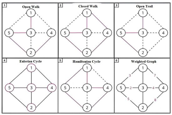
Figure 1.
Example—graph theory. (1) Open Walk—A sequence of vertices and edges where the first and last vertex can be different, and vertices and edges may be repeated. (2) Closed Walk—A sequence that starts and ends at the same vertex, allowing repetition of vertices and edges. (3) Open Trail—A sequence of vertices and edges where edges are not repeated, but vertices may be. The first and last vertex can be different. (4) Eulerian Cycle—A cycle that traverses every edge of the graph exactly once and returns to the starting vertex. (5) Hamiltonian Cycle—A cycle that visits every vertex of the graph exactly once and returns to the starting vertex. (6) Weighted Graph—A graph where each edge has an associated weight, representing cost, distance, or another metric. Source: authors, 2024.
2.2. Ant Colony Optimization (ACO)
The Ant Colony Optimization (ACO) metaheuristic, a nature-inspired approach, emulates the collective behavior of ants searching for food. In this process, ants leave their anthill (starting point) and navigate toward food sources, optimizing their paths by evaluating multiple routes through indirect communication via pheromones, as depicted in Figure 2. The image demonstrates the use of the ACO metaheuristic to identify the optimal locations for service stations along highways, aiming to maximize user reach while balancing economic reliability factors by comparing the current and ideal positions.
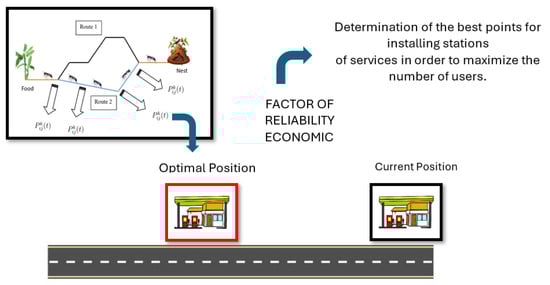
Figure 2.
Example of ant behavior. Source: Authors, 2024.
Understanding the overall structure of the ACO algorithm provides the necessary foundation for exploring its mathematical components, which formalize decision-making processes and refinement of solutions. Among these components, the probability formula plays a central role, since it guides the artificial ants in choosing the edges during the construction of the solutions. The probability formula in the ACO algorithm is used to determine the chance of an ant choosing an edge (vi, vj) when building its solution. This probability is influenced by two main factors: the pheromone level at the edge, which represents the accumulated experience of previous ants, and the local heuristic, which measures the immediate attractiveness of the path based on criteria such as distance or cost, as shown in Equation (1).
where
Pkij(t) = {[τij]^α [ηij]^β/∑l∈Nki(t) [τil]^α [ηil]^β, if j ∈ Nki(t); 0, otherwise.
- Pij = probability of an ant selecting the edge (vi, vj) as the next chosen path.τij = pheromone level present in the edge (vi, vj), indicating its attractiveness based on past experiences.
- ηij = heuristic information about the edge (vi, vj), usually represented as 1/dij, where dij is the distance between vertices vi and vj, indicating immediate attractiveness.
- α = parameter that controls the influence of the pheromone on the ant’s decision. Higher values of α favor more explored paths.
- β = parameter that controls the influence of the heuristic on the decision. Higher values of β favor shorter or lower-cost paths.
- k = set of vertices that are visible or accessible from the vertex (vi) that the ant (k) has not yet visited.
- sum of the pheromone and heuristic combinations for all edges visible from vertex i, ensuring that the probability is normalized (sum equal to (1)).
This equation balances the exploration of new paths (guided by heuristics) with the exploitation of already explored routes (influenced by pheromone), allowing the algorithm to build optimized solutions iteratively and adaptively. Updating the pheromone is a crucial step in the ACO algorithm, as it directly influences the future decisions of the artificial ants when building solutions. This process occurs after each iteration of the algorithm and aims to adjust the pheromone levels at the edges of the graph based on the quality of the solutions found. The edges that make up the best routes receive pheromone increments, reinforcing their attractiveness, while the rest of the edges undergo a pheromone reduction due to the evaporation process. This dynamic allows the algorithm to balance the exploration of new routes and the exploitation of already explored routes, preventing stagnation at local minima and guiding the convergence to high-quality solutions [11,12].
The update of the pheromone levels of edge (vi, vj) is expressed by Equation (2):
where
- ρ is the evaporation rate (0 < ρ < 1).
- τij is the pheromone level at the edge (vi, vj) after updating (1 − ρ). This step reduces pheromone levels, preventing all ants from following unique routes and encouraging the exploration of new solutions.
- Δτij is the increment in the pheromone deposited by ants that traveled the edge (vi, vj) during iteration t, calculated as Equation (3):
- Q is the total amount of pheromone deposited.
- Ck is the cost of the solution generated by the k-th ant (for example, the total distance traveled).
Pheromone updating plays a central role in the progress of the ACO algorithm, guiding the construction of solutions throughout iterations and continuously adjusting the attractiveness of routes. However, to ensure that the algorithm operates efficiently, avoiding unnecessary or excessively long executions, it is essential to establish well-defined stop criteria. These criteria determine when the iterative process should be stopped, either based on a maximum number of iterations, execution time, or convergence of solutions, ensuring a balance between quality of responses and computational cost [11,12]. The most common criteria include the maximum number of iterations, execution timeout, and convergence of solutions. In the case of convergence, the algorithm is interrupted when the pheromone levels and the generated solutions do not show significant changes between consecutive iterations, indicating that the exploration of the search space has been sufficiently saturated. Moreover, problem-specific constraints such as resource limits or time requirements can be incorporated as additional stop conditions.
The stop criteria in the ACO algorithm can be formulated mathematically to reflect the specific conditions under which the algorithm must stop its execution. We present below some of these stop criteria used by the algorithm.
Maximum number of ants: This criterion interrupts the algorithm after a predefined number of iterations and can be exemplified by k ≤ Nmax, where k is the current ants of the algorithm and Nmax is the predefined maximum number of iterations.
Timeout: This criterion is used to determine a maximum execution time Tmax, at which the algorithm must stop when the total time Texec exceeds the limit, Texec ≤ Tmax.
Convergence of solutions: The convergence criterion is based on the stabilization of the pheromone level or the absence of significant improvements in the solution over a number of consecutive iterations.
Despite being widely recognized for its efficiency in combinatorial optimization problems, the ACO metaheuristic has some limitations. The main ones include the possibility of premature convergence, where the pheromone is excessively concentrated in a few routes, leading to suboptimal solutions, in addition to sensitivity in the configuration of parameters, such as α, β, and ρ. These factors can make the initial adjustment challenging, especially in large-scale problems where computational cost becomes significant [11,12].
The ACO metaheuristic, initially applied to the Traveling Salesman Problem, stands out for its efficiency in optimizing lower-cost cycles in complete graphs, where the vertices represent cities and the edges indicate the paths with associated costs, such as distances or travel times. This method uses the systematic exploration of the routes in the graph to find efficient solutions, simulating the collective behavior of ants. The ability to solve problems like this shows the flexibility of the technique, which serves as the basis for its application in more complex challenges, such as the Vehicle Routing Problem (VRP), where multiple vehicles and additional restrictions are incorporated. Therefore, the ant colony evolves from a solution to a classical problem to a robust approach in graph-based logistics optimization [11,12]. Similarly, Hu et al. (2014) [13] proposed an algorithm combining support vector regression (SVR) and particle swarm optimization (PSO) for traffic flow prediction. Their approach uses SVR to establish the prediction model while PSO optimizes its parameters. Tested on actual traffic data, the integrated method demonstrated superior performance compared to multiple linear regression and backpropagation neural networks, highlighting the effectiveness of hybrid metaheuristics in traffic management applications. More recently, Akopov et al. (2025) [14] introduced a hybrid evolutionary algorithm (MA-HCAGA) to optimize topologies of Reconfigurable Multilayer Road Networks (RMRNs), balancing vehicle flow and structural complexity.
2.3. Formulation of the Vehicle Routing Problem (VRP)
VRP has its roots in TSP. For this reason, its mathematical formulation also follows similar parameters, preserving, however, the particularities that make it a more effective problem to current requests. The original formulation proposed by Dantzig (1959) [15] and adapted by Silva (2024) [16], presented below, illustrates the objective function of minimizing the cost of a trip carried out by a number of cars from the point of origin (warehouse) to the point of destination (delivery to the customer) and their respective restrictions.
- Objective function:
Given a graph G, with a set of vertices V (delivery points) and with a set of edges E (cost for the path between two points) connecting them, and that enables a trip of a set of vehicles K, Equation (4) shows the proposed minimization function:
Restrictions:
- 1.
- ;
- 2.
- ;
- 3.
- ;
- 4.
- ;
- 5.
- ;
- 5.
- ui − uj +n n−1,.
where
- Z = cost minimization function for a delivery route;
- i,j = origin–destination pair of vertices of each route analyzed in the solution iterations;
- Cij = cost of moving between vertices i and j;
- K = any vehicle that travels the distance between i and j;
- = cost-bound binary constraint function with the objective of verifying the travel of k to i and j; 1 for yes, 0 for no.
- Ui = continuous variable representing the position of node i in vehicle k route, helping to prevent subtours.
Restriction 1 is used to ensure that each customer is visited only once, by a single vehicle on a single route; the restriction is valid for all points from 1, which excludes the warehouse (point of origin), assigned a value of 0 [16].
Restriction 2 limits that each vehicle must depart from the warehouse to the destination point only once, ensuring that all routes taken during iterations are closed, i.e., starting and ending at the same point [16].
Restriction 3 limits that each vehicle must return to the warehouse only once, ensuring that all routes taken during iterations are closed, i.e., starting and ending at the same point [16].
Restriction 4 is applied to the problem to ensure that the movement flow is maintained throughout the path simulation. Therefore, the quantity of vehicles leaving the warehouse must be equal to the quantity arriving at the warehouse [16].
Restriction 5 relates the customer’s demand to the capacity of the vehicle that will serve them. Therefore, if a vehicle has a lower capacity than requested, it is not used for the route in question [16].
Restriction 6 serves to eliminate subcycles. As seen in the formulation of TSP, VRP also has a constraint that seeks to eliminate possible subcycles created during iterations. Thus, it is ensured that only connected routes are created for each of the vehicles [16].
Each vehicle must form a single continuous route, starting and ending at the depot, without creating smaller cycles that exclude the depot or other customers that should be visited.
The global solution must prevent the formation of groups of customers served in independent cycles that are not connected to the rest of the route.
3. Related Works
The methods discussed earlier (exact, non-exact, and heuristic) can also be applied to VRP, provided that the necessary adaptations are made to meet the specificities of the problem. In general, exact algorithms are used for smaller instances, while non-exact methods, including heuristics and metaheuristics, are preferred for more complex or large-scale problems, where the search space exceeds the computational capacity of the exact methods.
Among the non-exact methods widely applied to VRP, we highlight the ACO algorithm, a metaheuristic inspired by the behavior of ants in the search for food. Its use in VRP is encouraged by several advantages, such as effectiveness in finding approximate solutions to combinatorial optimization problems. This is due to its ability to explore the search space and refine solutions interactively, as well as to easily adapt to variations in the problem, such as time windows and multiple warehouses.
4. Methodology
This section highlights the methodology employed in this work. The stage of an ACO metaheuristic for a classic VRP is considered in Figure 3.
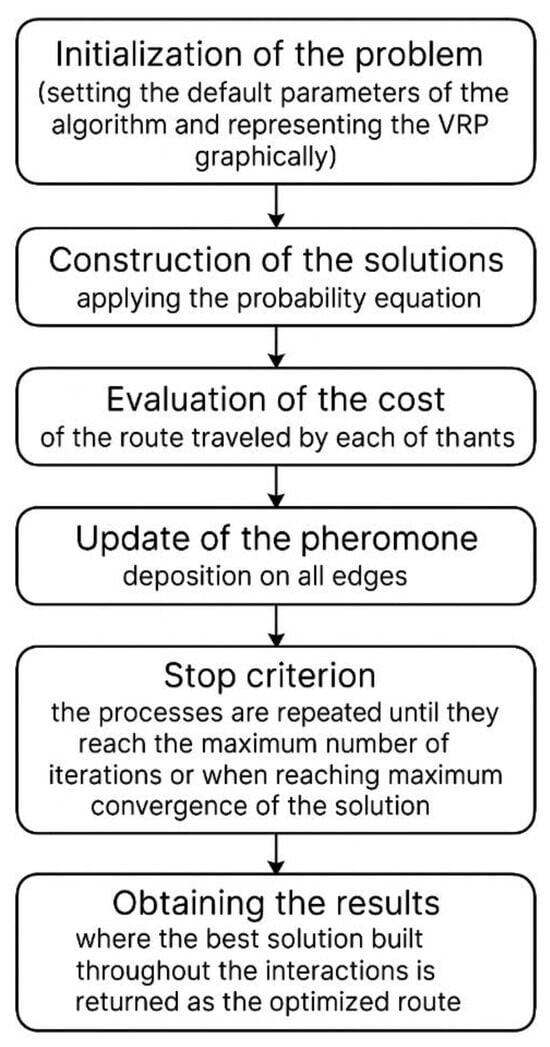
Figure 3.
Flowchart of the methodology. Source: Authors, 2024.
4.1. Application of the ACO Metaheuristic in the Allocation of Service Stations on Highways
The model was developed in Python based on the modeling of the proposed scenario using the stages of the ACO metaheuristic, adapting it to the concepts of Transport Engineering, seeking a comparison between the points already built and those provided by the study method defined in Equation (5).
where
- ρ∈0,1: parameter regulating the reduction of τij(t);
- τij(t): intensity of the pheromone present at the edge (i,j) at the t-th iteration;
- Q: amount of pheromone deposited by an ant for an entire solution;
- RL: real distance;
- RO: optimal distance.
From Equation (5), the parameters were adjusted to the variables intrinsic to Transport Engineering, as presented in Table 1.

Table 1.
Correlation between the theoretical parameters of the ACO metaheuristic and Transport Engineering.
In the Ant Colony Optimization (ACO) framework, Equation (5) defines an adjusted parameter linking pheromone reinforcement to key ACO variables. Here, given by an equation such as Equation (2), represents the updated pheromone level on edge (vi,vj), with as the evaporation rate and Δτij as the deposited pheromone (often ). The denominator measures the net pheromone increase beyond a persistence-adjusted baseline . Thus, the ratio normalizes (Q) against the difference, dynamically adjusting pheromone reinforcement. A larger reduces , indicating weaker reinforcement, while a value close to increases it, enhancing sensitivity.
The description of this study, involving the route between Limeira and São Paulo via the Bandeirantes Highway (SP348), proposes an analysis related to logistics and transport system planning, a context in which ACO is often applied. Figure 4 depicts the route calculated in this study.
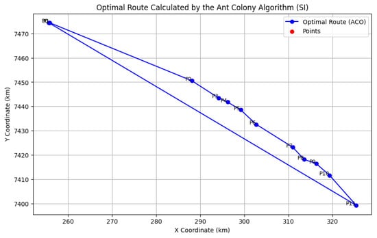
Figure 4.
The 12 points collected from Bandeirantes Highway SP348. Source: Authors, 2024.
The described approach considers the optimization of the choice of gas stations along the route, a task analogous to classical routing problems. In this scenario, the algorithm can be modeled so that the ants represent simulated vehicles that travel the route, depositing pheromones at the stations that best meet the established conditions, such as energy efficiency and proximity to the fuel or battery capacity limit. These decision points (gas stations) can be treated as nodes of a graph, where ants choose paths based on probabilistic criteria associated with characteristics such as distance, remaining energy, and accumulated pheromone intensity.
The adjustable parameters described in this study, such as pheromone decay and energy consumption per kilometer, are directly related to the elements of ACO. Decay control, for example, reflects the volatility of pheromone trails, allowing the algorithm to maintain a balance between exploring new solutions and intensifying around the most promising routes. Similarly, energy consumption per kilometer can be included as a constraint or a decision factor in the model, affecting the ants’ simulated choices.
In the context of ACO, a system with high entropy would be associated with a broad exploration of the solution space, avoiding early convergence to an optimal location. Thus, entropy provides an indicator of the quality of the search performed by the algorithm. The proposal to test different scenarios in the study, such as changes in traffic patterns or variations in operational parameters, aligns with the flexibility of ACO to adapt to different input conditions.
The practical application of ACO to the problem of the highway may involve the identification of the best gas stations throughout the route, considering both the minimization of travel time and the maximization of energy efficiency. In addition, the model can be adjusted to incorporate real constraints, such as the proximity of stations to the carriageway, contributing to the achievement of viable solutions in the context of road transport. Nevertheless, the study shows how ACO can be an effective tool to address challenges related to logistics and optimization in transportation systems.
4.2. Modeling Freight Costs: A Contemporary Integration of Physics, Regression, and Entropy
Modeling freight costs is a complex challenge requiring the integration of spatial, temporal, and economic variables, often grounded in physical analogies and advanced statistical methods. This study proposes an interdisciplinary framework combining Newtonian dynamics, gravitational models, linear regression, and entropy, aligning with recent trends in transportation and logistics research. A gravitational analogy is introduced in Equation (6), adapted from [17]; this formulation is refined by [18] for transportation modeling. Solving for ,
where
- Tij is the freight flow;
- Pi and Pj represent population in the zones (e.g., cargo volume), and dij is the distance.
Using time as an independent variable, Equation (7) can be used to model the money-related variable.
where
- y(t): money-related variable at time t;
- : variable of space with time;
- : intercept, representing the y value when x is zero;
- : coefficient associated with the time variable;
- : Factor Error.
Freight cost Cf is modeled using linear regression [19]. Transforming Equation (7) for the cost of freight, we obtain Equation (8)
where uncertainty in ϵt is analyzed via conditional entropy. Using entropy can be explored in the context of information theory, as in Equation (9):
where
Cf = β0 + β1.dist(1) + β2.timeTraffic + ϵt
H(ϵt|Distance, timeTraffic) = −E[log P (ϵt|Distance, timeTraffic)]
H is the conditional entropy of the error variable ϵt with the knowledge of the distance and traffic time;
P (ϵt|Distance, timeTraffic)] regression represents the relationship between freight cost, distance, and traffic time;
dist(1) refers to the distance traveled in a specific unit (e.g., kilometers or miles), typically the physical distance between two points, such as the origin and the first destination (indicated by “(1)”). In the context of “distance traffic” (traffic distance), it may represent the effective distance on a route subject to traffic conditions.
|Distance, timeTraffic represents the time spent in traffic, measured in units such as minutes or hours. This term captures the effect of traffic conditions (congestion, average speed, etc.) on the total cost. In the context of “distance traffic”, it refers to the additional or variable time associated with the distance traveled in a traffic-affected environment.
E is the economic reliability factor.
In Equation (9), H measures residual uncertainty, and E[log P (ϵt|Distance, timeTraffic)] is the expectation. This aligns with modern applications in transportation [20] for modeling flow uncertainties.
- The differential entropy H(ϵt) = ) depends exclusively on the variance σ2, reflecting that the uncertainty of a normal distribution increases with the dispersion of values. The constant terms 2π (e) emerge from the structure of the Gaussian:
- 2π is related to the normalization constant of the PDF.
- e: (the base of natural logarithms) reflects the property of the normal distribution as the maximum entropy distribution for a fixed variance.
- It should be noted that H(ϵt) can be negative for σ2 < , a typical behavior of differential entropy, which is not lower-bounded like discrete entropy.
The entropy of ϵt can be estimated as in Rashedi et al. [20], assuming ϵt~N (0,):
This framework introduces an innovative approach to freight transport cost modeling, integrating principles of physics, economics, and information theory, grounded in the recent literature. It contributes to advancements in Transport Engineering and logistics, emphasizing the need for empirical validation to enhance mobility systems and operational efficiency.
5. Results and Discussion
As described, values considered appropriate for popular Brazilian vehicles were used to obtain the results and are thus considered the standard vehicles in this study. The variation in the yield/range values is adopted to verify the behavior of the results, while the other parameters remain fixed:
Q = 47 Liters (tank capacity of a passenger vehicle), and τij(t) = 10% of tank capacity (minimum fuel level in the tank for refueling to occur).
The relationship between the economic reliability factor (ERF) and fuel efficiency is established based on the difference between the estimated optimal value and the real value obtained. Such a difference reflects the accuracy and reliability of the economic model in predicting fuel consumption performance under practical conditions and is an essential indicator for assessing the efficiency of projected results and their adherence to real operating conditions. This relationship is directly linked to fuel efficiency indices, as higher performance values result in a proportional reduction in standard deviations in economic reliability factors, as shown in Figure 4. This provides a more precise and accurate analysis of fuel efficiency.
An important consideration when employing the Ant Colony Optimization (ACO) metaheuristic is its effectiveness in solving problems that involve cost minimization or maximization, such as fuel consumption evaluation. By simulating the collective behavior of ants and employing a pheromone updating mechanism, ACO is capable of exploring a variety of solutions aimed at improving fuel efficiency. In this context, the objective is to enhance performance while reducing the variability of economic factors in transportation systems.
In order to achieve this, the algorithm must be calibrated based on the values obtained from Equation (2), prioritizing solutions that exhibit both a higher standard deviation of the Economic Risk Factor (ERF) and improved fuel efficiency.
Accordingly, the search process favors solutions that yield higher performance and lower ERF variability, thereby contributing to the continuous improvement of system efficiency. The employed algorithm enables the exploration of new configurations, as well as the iterative refinement of previously identified solutions, aiming to achieve a balance between innovation and optimization.
In this scenario, the logarithmic regression that models the relationship between yield and ratio serves as a guide to adjust preferences, guiding the system towards a convergence of more sustainable and economically efficient solutions.
The ACO metaheuristic not only complements ERF analysis but also provides a powerful tool for optimizing complex efficiency and economic problems.
Table 2 and Figure 4 show the results of the analysis of the RL/(RO ratio, fundamental for the calculation of the optimal x coordinate, considering the coordinates of the gas stations collected along the Bandeirantes Highway and the standard fuel yields of vehicles from the Brazilian popular fleet. The table presents the values of the standard deviation of the RL/OL ratio for each level of fuel efficiency, analyzed in a range from 5 km/L to 20 km/L. Figure 4 graphically illustrates this relationship, showing a direct correlation between the standard deviation and fuel yield. It appears that this relationship can be applied to achieve good allocation results in two ways: (i) data collection for a more robust set of information, which implies a decrease in the standard deviation; (ii) stations with more frequent access of vehicles with a greater range can be reflected in the final result of the solution (ideal solution).
Table 2.
Application of different yield values.
Figure 5 shows the standard deviations of the different yield values and their regression line.
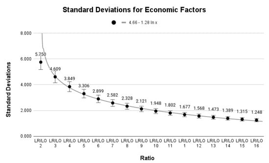
Figure 5.
Standard deviations of the different yield values and their regression line. Source: Authors, 2024.
5.1. Optimizing Freight Transport Routes Using Ant Colony Optimization: A Multi-Faceted Approach with Distance, Cost, and Entropy Analysis
This pseudocode implements an Ant Colony Optimization (ACO) metaheuristic to determine the most efficient freight transport route between Limeira and São Paulo, considering fuel constraints and intermediate stops along the SP-348 highway. The algorithm minimizes travel distance while accounting for refueling needs, using pheromone-based decision-making. Additionally, it calculates freight flow based on a gravitational model, estimates transport costs as a function of distance and traffic time, and computes entropy to assess variability. The accompanying visualizations include a map of the optimized route with labeled stops (Figure 6), a bar chart comparing real versus optimized distances (Figure 7), a curve showing freight cost as a function of distance with the optimized point highlighted (Figure 8), and an entropy plot illustrating the relationship between error variance and system uncertainty, emphasizing the chosen variance value (Figure 9).
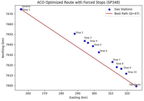
Figure 6.
Optimized route by the ACO metaheuristic. Source: Authors, 2024.
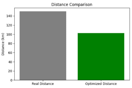
Figure 7.
Distance comparison. Source: Authors, 2024.
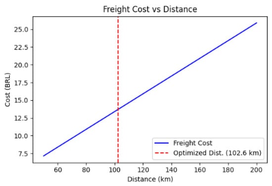
Figure 8.
Freight cost as a function of distance. Source: Authors, 2024.
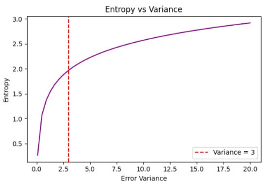
Figure 9.
Entropy as a function of error variance. Source: Authors, 2024.
Initialize parameters: α, β, ρ, Q, number of ants, and pheromone levels τ
While stopping condition not met do:
For each ant do:
Construct a solution (route) based on τ and heuristic η
end for
Evaluate all constructed solutions
Update pheromone trails:
τ ← (1 − ρ) × τ + Δ τ (from best solutions)
Store best global solution
end while
Return best solution found
Figure 6 presents the spatial representation of the optimized route. In this figure, the points indicate the locations of refueling stations along the route, while the line illustrates the path identified by the ACO algorithm. This representation allows us to verify that the metaheuristic selected intermediate stations to optimize fuel consumption and minimize travel costs.
Figure 7 provides a comparative analysis of the direct distance between Limeira and São Paulo versus the final distance obtained through the ACO algorithm. In this bar chart, the actual real-world distance between the two cities is represented by a gray bar, while the optimized route distance calculated by ACO is shown in green.
The x-axis categorizes these two distances as follows: “Real Distance”, which corresponds to approximately 150 km, and “Optimized Distance”, which is significantly shorter (e.g., 76.12 km). The y-axis measures distance in kilometers.
This difference arises because the optimized distance is calculated using Euclidean distances based on UTM coordinates, which only consider straight-line measurements between given points. As a result, the ACO algorithm underestimates the actual length of the SP-348 highway. This suggests two possible explanations: (1) the provided waypoints represent only a partial segment of the highway, or (2) the ACO algorithm prioritizes the shortest possible route since it assumes that vehicles have sufficient fuel autonomy and do not require additional detours for refueling.
This graph highlights a key limitation of the model: the simplified spatial representation does not fully capture the real-world road network, which includes curves, junctions, and other logistical constraints.
Figure 8 relates the traveled distance to the freight cost. The blue curve represents the variation in transportation costs as the distance increases, following a fitted linear model. The vertical red line marks the distance optimized by ACO, indicating where the proposed solution falls within the cost function. This graph reinforces that, despite a slight increase in total distance, optimization can lead to cost reductions by avoiding excessive fuel expenses and unplanned stoppages.
Figure 9 examines the behavior of system entropy as a function of error variance (εt). The purple curve represents the increase in entropy as the variability in transport costs rises. The vertical red line indicates the standard error variance value (εt = 3).
The graph shows that data variability is directly associated with increased uncertainty in transportation costs, reinforcing the need to reduce fluctuations and seek greater predictability in the logistics decision-making process.
The analysis of the graphs indicates that the application of the Ant Colony Optimization (ACO) metaheuristic contributes to route optimization by considering factors such as fuel consumption and operational costs. The algorithm identifies routes that balance energy efficiency and economic viability, not necessarily favoring the shortest path. Table 2 showcases a comparison between ACO and generic algorithms.
Moreover, the modeling of costs and entropies in relation to financial predictability, combined with the appropriate definition of constraints, allows for a more accurate calibration of the algorithm based on real-world activity data, thereby enhancing its practical relevance.
5.2. Benchmark Comparison with Generic Algorithms
To validate the effectiveness of the Ant Colony Optimization (ACO) model, we conducted a comparative analysis with two generic algorithms commonly used in routing problems: Dijkstra’s shortest path algorithm and the Nearest Neighbor heuristic. These benchmarks were chosen due to their simplicity, wide usage in classical optimization problems, and ability to provide a reference for evaluating the added value of ACO. Table 2 summarizes the results. While Dijkstra and Nearest Neighbor focus on geometric proximity and greedy choices, respectively, ACO integrates dynamic constraints such as fuel range and pheromone memory. As shown in Table 3, ACO achieved a significantly shorter total path (76.12 km), compared to 102.60 km with Dijkstra and 104.53 km with Nearest Neighbor.
Table 3.
Comparison between ACO and generic algorithms.
The capability of Ant Colony Optimization (ACO) to address complex logistical challenges is clearly demonstrated in this study. This research provides an innovative and relevant contribution to the management of complex logistics operations. The comparison reinforces the applicability of the ACO model in real-world logistics scenarios, particularly in optimizing fuel supply chains for road transport systems. This approach becomes even more strategic in the context of electric vehicles, where efficient placement of charging stations is essential to ensure route feasibility and operational optimization, enabling more informed and effective decision-making for logistics managers.
5.3. Sensitivy Analysis
Given the relevance of the parameters that govern the behavior of the Ant Colony Optimization (ACO) metaheuristic, particularly α (relative importance of the pheromone trail), β (relative importance of the heuristic information), ρ (pheromone evaporation rate), and Q (pheromone deposit intensity), it is essential to investigate the model’s sensitivity to variations in these elements. As highlighted by the reviewer, the initial absence of a sensitivity analysis could compromise the understanding of the algorithm’s robustness and stability.
Accordingly, this section presents a sensitivity analysis aimed at evaluating the individual impact of each parameter on the optimization model’s performance, in terms of both solution quality and convergence rate. This approach is fundamental not only for justifying the choices made during the algorithm’s calibration but also for demonstrating the consistency of the results under different parameter configurations. In this context, the analysis considers the 12 optimization results (RO) obtained by the method, which serve as the basis for assessing the effects of parameter variation. The following subsections present the observed effects of varying each of the four analyzed parameters.
The first parameter to be modified was ρ (pheromone evaporation rate). In this case, values ranging from 20 to 5 were analyzed (15 different scenarios), representing the average fuel consumption in kilometers per liter. The results indicate that as the average fuel efficiency decreases (i.e., below 15 km/L), the optimization result tends to increase when compared to the previously obtained reference result. Conversely, when fuel efficiency remains above this threshold, the optimization result tends to be lower than the reference result.
With respect to the pheromone trail parameter τij, the sensitivity analysis reveals that when its value is below 0.1 (specifically in the range of 0.025 to 0.075), the difference in the obtained solution (PO) compared to the previous result tends to be minimal. However, as τij increases beyond 0.1 (ranging from 0.125 to 0.525), the value of PO tends to increase in comparison to the previous result, with variations ranging from 0.16 to 3.43 units, corresponding to a relative increase between 0.057% and 0.0981%. These findings suggest that higher pheromone trail values may lead to less efficient solutions, likely due to excessive reinforcement of early paths, thereby reducing the algorithm’s exploratory capacity.
Regarding the vehicle’s fuel tank capacity parameter Q, the sensitivity analysis indicates that capacities ranging from 35 to 46 L tend to produce higher optimization results compared to the current baseline case, with increases ranging from 0.078% to 0.005%. In contrast, when the tank capacity exceeds 47 L, the optimization results tend to be lower than the baseline, with variations between 0.005% and 0.033%. These outcomes suggest that increasing the tank capacity beyond the baseline may enhance route efficiency by reducing the number of required refueling stops, while lower capacities may constrain route planning and increase overall costs.
This sensitivity analysis highlights the crucial role that parameter calibration plays in the performance of the ACO algorithm. Variations in ρ, τij, and Q demonstrated measurable impacts on solution quality, reinforcing the need for careful parameter tuning to ensure algorithmic robustness. The observed trends confirm that suboptimal parameter values can lead to performance degradation, while appropriate adjustments can enhance efficiency. Therefore, sensitivity analysis is not only a diagnostic tool but also a guiding step in model refinement. These insights support the validity of the chosen configuration and contribute to the reliability of the optimization results.
6. Conclusions
This study demonstrated the effectiveness of the Ant Colony Optimization (ACO) metaheuristic in solving problems related to Vehicle Routing and service station allocation, offering more robust and adaptable solutions for complex logistics challenges. The introduction of the economic reliability factor (ERF) represented a significant advance in route analysis, enabling a more accurate assessment of the economic and operational feasibility of the proposed solutions. The practical application on the Bandeirantes Highway illustrated the flexibility of the model, reinforcing the potential of ACO in real-world transportation contexts.
Despite these contributions, this study presented limitations regarding the use of Python for complex simulations, pointing to the need for more advanced computational tools capable of handling large-scale modeling. Moreover, integrating ACO with other metaheuristics or machine learning algorithms emerges as a promising direction to further improve solution quality and extend the methodology’s applicability.
In particular, the hybridization of ACO with reinforcement learning (RL) has shown notable effectiveness in addressing optimization problems such as Vehicle Routing Problems (VRPs), enabling algorithms to dynamically adapt their search behavior and improve convergence in complex, dynamic environments. This perspective aligns with a recent work [21] which emphasized that the growing complexity and real-time demands of manufacturing scheduling problems characterized by large scale, high interdependence, and multiple conflicting objectives require intelligent hybrid approaches. The review highlights how the synergy between metaheuristics and reinforcement learning plays a critical role in enhancing decision-making through ensemble methods, adaptive criteria, and real-time feedback mechanisms.
The findings of this study reinforce the relevance of ACO as a powerful tool for Transport Engineering, with wide potential applications across logistics and road infrastructure sectors. Future research should explore the development of hybrid algorithms such as ACO-RL frameworks, the use of real-time operational data, and the adaptation of the model to both urban and rural scenarios, thus consolidating ACO’s role as an efficient and sustainable solution to contemporary logistics and mobility challenges.
Author Contributions
Conceptualization, Y.A.M.; Methodology, F.P.L.d.S., G.d.G.; Software, W.M.E.; Validation, F.B.C., V.E.M.J., J.R.B.J.; Formal analysis, F.B.C. and V.E.M.J.; Investigation, F.P.L.d.S.; Resources, Y.A.M.; Data curation, F.P.L.d.S., G.d.G.; Writing—original draft preparation, L.V.F.d.M.F.; Writing—review and editing, J.R.B.J. and Y.A.M.; Visualization, W.M.E.; Supervision, Y.A.M.; Project administration, Y.A.M.; All authors have read and agreed to the published version of the manuscript.
Funding
This research received no external funding.
Data Availability Statement
Data will be available on request.
Acknowledgments
The authors thank Espaço da Escrita—Pró-Reitoria de Pesquisa—UNICAMP—for the language services provided.
Conflicts of Interest
The authors declare that they have no conflict of interest.
References
- Aveni, A. Os desafios logísticos e as tendências em relação ao chamado e-commerce. Rev. JRG De Estud. Acadêmicos 2019, 2, 71–83. Available online: https://www.revistajrg.com/index.php/jrg/article/view/124 (accessed on 5 September 2024).
- Mukai, H.; Dias, S.I.S.; Feiber, F.N.; Taboada Rodriguez, C.M. Urban logistics. In Proceedings of the 27th National Meeting of Production Engineering (ENEGEP), Foz do Iguaçu, Brazil, 9–11 October 2007. [Google Scholar]
- Souza, N.L.S.; Silva, M.R.F.; Taboada, C.M.; Frazzon, E.M. Tendências e indicadores de desempenho logístico da última milha: Uma revisão de literatura. In Encontro Nacional de Engenharia de Produção, 42; Anais, Ed.; ABEPRO: Foz do Iguaçu, Brazil; Rio de Janeiro, Brazil, 2022; Available online: https://abepro.org.br/biblioteca/TN_ST_383_1895_43920.pdf (accessed on 5 September 2024).
- Elatar, S.; Abouelmehdi, K.; Riffi, M.E. The vehicle routing problem in the last decade: Variants, taxonomy and future directions. Procedia Comput. Sci. 2023, 220, 398–404. Available online: https://www.sciencedirect.com/science/article/pii/S1877050923005860 (accessed on 1 October 2024). [CrossRef]
- Nielsen, P.; Dahanayaka, M.; Perera, H.N.; Thibbotuwawa, A.; Kılıç, D.K. A systematic review of vehicle routing problems and models in multi-echelon distribution networks. Supply Chain Anal. 2024, 1, 100072. [Google Scholar] [CrossRef]
- Luzia, L.F.; Rodrigues, M.C. Estudo Sobre as Metaheurísticas; Instituto de Matemática e Estatística, Universidade de São Paulo: São Paulo, Brazil, 2009. [Google Scholar]
- Becceneri, J.C. Meta-heurísticas e otimização combinatória: Aplicações em problemas ambientais. Rev. Bras. Comput. Apl. 2010, 2, 1–15. [Google Scholar]
- Ostrowski, K.; Starzec, M.; Starzec, G. The Ant Colony Optimization Algorithm Applied in Transport Logistics. Comput. Sci. 2024, 25, 221–238. [Google Scholar] [CrossRef]
- Diestel, R. Graph Theory, 6th edSpringer: Springer: Berlin/Heidelberg, Germany, 2025. [Google Scholar]
- Chen, J.; Li, C.H.; Praeger, C.E.; Song, S.J. The graphs with a symmetrical Euler cycle. arXiv 2021, arXiv:2111.02615. [Google Scholar]
- Toledo, F. Metaheurísticas Baseadas em Trajetória e População Para Problemas de Roteamento de Veículos. Ph.D. Thesis, Universidade de São Paulo, São Paulo, Brazil, 2019. [Google Scholar]
- Lopes, M.J. Heurísticas e Meta-Heurísticas Aplicadas ao Problema de Roteirização de Veículos. Master’s Thesis, Universidade Federal do Paraná, Curitiba, Brazil, 2008. [Google Scholar]
- Hu, W.; Yan, L.; Liu, K.; Wang, H. A Short-Term Traffic Flow Forecasting Method Based on the Hybrid PSO-SVR. Neural Process. Lett. 2016, 43, 155–172. [Google Scholar] [CrossRef]
- Akopov, A.S.; Beklaryan, L.A. Evolutionary Synthesis of High-Capacity Reconfigurable Multilayer Road Networks Using a Multiagent Hybrid Clustering-Assisted Genetic Algorithm. IEEE Access 2025, 13, 53448–53474. [Google Scholar] [CrossRef]
- Dantzig, G.B.; Ramser, J.H. The truck dispatching problem. Manag. Sci. 1959, 6, 80–91. Available online: https://www.jstor.org/stable/2627477 (accessed on 1 October 2024). [CrossRef]
- Silva, R.A. Algoritmos Evolutivos Híbridos com Detecção de Regiões Promissoras em Espaços de Busca Contínuos e Discretos. Master’s Thesis, Instituto Nacional de Pesquisas Espaciais, São José dos Campos, Brazil, 2004. [Google Scholar]
- Wilson, A.G. Entropy in Urban and Regional Modelling; Note: Included as a Historical Foundation, Widely Cited in Recent Works; Pion Limited: London, UK, 1970. [Google Scholar]
- Ortúzar, J.D.; Willumsen, L.G. Modelling Transport, 4th ed.; Wiley: Hoboken, NJ, USA, 2011. [Google Scholar] [CrossRef]
- Greene, W.H. Econometric Analysis, 8th ed.; Pearson Education: London, UK, 2018. [Google Scholar]
- Rashedi, M.R.; Zhang, K.; Mahmoudzadeh, H. Entropy-Based Models for Transportation Network Equilibrium. Transp. Res. Part B Methodol. 2017, 102, 14564. [Google Scholar] [CrossRef]
- Fu, Y.; Wang, Y.; Wang, Y.-F.; Gao, K.; Huang, M.; Chen, N. Review on ensemble meta-heuristics and reinforcement learning for manufacturing scheduling problems. Comput. Electr. Eng. 2024, 120, 109780. [Google Scholar] [CrossRef]
Disclaimer/Publisher’s Note: The statements, opinions and data contained in all publications are solely those of the individual author(s) and contributor(s) and not of MDPI and/or the editor(s). MDPI and/or the editor(s) disclaim responsibility for any injury to people or property resulting from any ideas, methods, instructions or products referred to in the content. |
© 2025 by the authors. Licensee MDPI, Basel, Switzerland. This article is an open access article distributed under the terms and conditions of the Creative Commons Attribution (CC BY) license (https://creativecommons.org/licenses/by/4.0/).