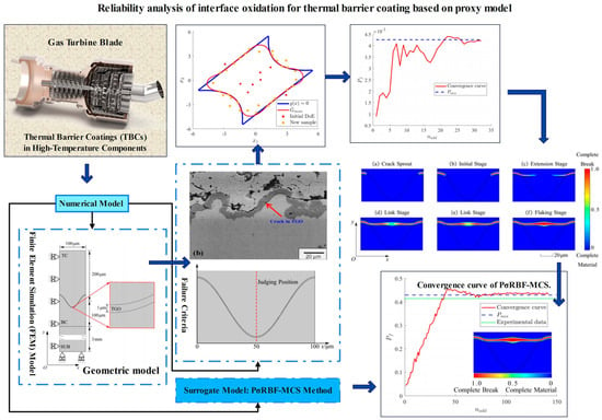
Reliability Analysis of Interface Oxidation for Thermal Barrier Coating Based on Proxy Model

Abstract

Thermal barrier coatings have been widely used in industrial fields where thermal damage occurs, and they are crucial for insulation technology and for the safe service of high-temperature components. So, it is critical to accurately predict the reliability of thermal barrier coatings. In this work, an adaptive reliability analysis method based on radial basis functions is proposed, in which different shape parameters and subsets are used to initiate different radial basis function models for multiple predictions. An active learning function that comprehensively considers local uncertainty, limit state function information, and distance among samples is then used for sequential sampling, and the proposed method is validated via a four-branch series connection system. Finally, a reliability analysis is conducted on the failure of interface oxidation in thermal barrier coatings, which verifies the feasibility of the proposed method.

1. Introduction

Thermal barrier coating (TBC) is a thermal protection technology that combines high-temperature resistant insulating ceramic materials with matrix materials to reduce the surface temperature of hot end components and improve the resistance of matrix materials to high-temperature oxidation and corrosion, thereby extending the service life of hot end components under high temperature and high stress conditions [1]. The TBC system can provide thermal insulation for turbine engine components, and protect them from harsh service environments such as isothermal oxidation, thermal corrosion, and thermal shock [2]. Thermal barrier coatings are commonly fabricated using various surface deposition techniques, each producing distinct microstructural characteristics. Among these, Atmospheric Plasma Spraying (APS) and Electron Beam Physical Vapor Deposition (EB-PVD) are the most prevalent [3]. APS results in a lamellar, porous microstructure with splat boundaries, which optimizes strain tolerance but may reduce durability under thermal cycling. In contrast, EB-PVD generates columnar microstructures that offer superior strain accommodation and thermal fatigue resistance [4]. The material composition also significantly influences performance: for example, coatings made with 8 wt% Yttria-Stabilized Zirconia (8YSZ) are favored for their low thermal conductivity and phase stability, whereas Gadolinium Zirconate (Gd₂Zr₂O₇) and La₂Zr₂O₇ offer improved sintering resistance and higher phase stability at elevated temperatures [5,6]. The interplay between deposition method and material selection thus plays a critical role in determining the long-term reliability and degradation behavior of TBC systems. In this study, a ceramic oxide-based top layer, an interfacial thermally grown oxide (TGO), a bond coat, and a substrate layer are modeled. The material properties used in the simulation are derived from the literature-reported values that represent a typical Atmospheric Plasma-Sprayed (APS) TBC system, selected for their industrial relevance and well-characterized thermomechanical behavior.

The harsh service environment in which TBC operates, however, often leads to interface peeling or thinning of the ceramic layer after a period of service, resulting in a decrease in its insulation performance and failure. Therefore, in order to ensure safety and utilization of TBC, it is necessary to propose a reliable analytical model for predicting its lifespan.

Due to the presence of various pores and microcracks in the microstructure of thermal barrier coating ceramic materials, material properties such as Young’s modulus, strength, fracture toughness, and thermal expansion coefficient are very dispersed. In addition, geometric shape, thermal characteristics, and load conditions often change and are unpredictable. After a period of high-temperature service, the thickness, microstructure, and shape of thermally grown oxide (TGO) layers will inevitably change, leading to changes in material properties. The uneven material properties, unstable microstructure, and variable working conditions make the service life of TBC full of uncertainty [7]. Nordhorn et al. [8] first applied the concept of reliability to TBC and obtained its failure probability based on finite element simulation, but did not consider the randomness of parameters, so the results obtained were limited. Guo et al. [9] considered the uncertainty of material properties and load parameters and analyzed the failure probability of TBC using first-order or second-order algorithms. However, TBC reliability is a high-dimensional and highly nonlinear problem, and the results obtained using first-order or second-order algorithms have a certain degree of errors.

In the reliability evaluation method based on the generalized stress intensity interference theory, the uncertainty parameters of the structure are concentrated in the design variables represented by X, and the reliability state of the structure is described by the function $g\left(X\right)$: when $g\left(X\right)>0$, it is a safe state; when $g\left(X\right)<0$, it is in a failure state; when $g\left(X\right)=0$, it is the Limit State Function. There are usually three types of structural reliability analysis methods: approximate analytical methods, numerical simulation methods, and surrogate model methods [10,11]. First-order and second-order reliability methods (FORM/SORM) are representative approximate analysis methods and can be replaced by low-order Taylor expansions [12]. However, for high-dimensional and highly nonlinear problems, some errors may occur in their estimated values. The traditional Monte Carlo Simulation (MCS) is a directly and widely used numerical simulation method in structural reliability analysis [13], but its accuracy depends on the size of a sample pool.

In addition, surrogate models or meta models can be seen as maximum structural response predictors, which are typically linear combinations of polynomials [14]. Compared with other structural reliability analysis methods, by combining surrogate models with sequential sampling, a small number of sampling points can be used to approximate the limit state gradually, so surrogate models receive more attention. At present, commonly used surrogate models include the Kriging model [15], support vector machine [16,17], artificial neural network [18,19], and response surface methodology [20,21]. However, there are relatively few structural reliability analysis methods based on radial basis function (RBF). In fact, the RBF method is easy to implement, has the characteristics of fast convergence, high prediction accuracy, and is suitable for high-dimensional problems [22,23].

In addition, the same sample can be predicted by using different surrogate models based on the multiple-prediction method in which different models can be constructed through linear combination so that better prediction results can be obtained, and the prediction variances of multiple predictions can to some extent measure the local uncertainty of the models. In recent years, there have been some related works based on multiple-prediction RBF methods. Shi et al. [24] proposed two adaptive models, VRBF-MCS and ARBFM-MCS, when considering the effects of different kernel function types and cross-validation subsets. Hong et al. [25] proposed a multi-prediction model that combines cross-validation and Jackknifing methods. The MSRBF-MCS proposed by Du et al. [26] considers the influence of kernel function shape parameters on sequential sampling, achieving a balance between efficiency and accuracy. However, these works based on RBF models have not comprehensively considered the influence of shape parameters and variance on local uncertainty.

In this work, an adaptive method is proposed based on the combination of the RBF model and MCS (Predicted Variance RBF-MCS method, i.e., P$\sigma$RBF-MCS method). Via the proposed method, the initial Design of Experiments (DoE) from Latin Hypercube Sampling is firstly generated and an initial meta model based on the initial DoE is constructed. Then, the optimal new sample points are selected from the Monte Carlo population through the proposed learning function, and the meta model is subsequently updated. In the proposed method, an RBF model for predicting lifespan is constructed by dividing DoE into multiple subsets and combining them with multiple shape parameters, and the local uncertainty of the model at new sample points is evaluated by using prediction variance. Moreover, a penalty function is used to maintain a certain distance between the new sample points and the existing DoE to avoid clustering problems. Finally, a four-branch series system example is used to validate the P$\sigma$RBF-MCS method, and the reliability evaluation of TBC interface oxidation failure based on the P$\sigma$RBF-MCS method is conducted to obtain its failure probability.

2. Surrogate Model Based on Radial Basis Function

2.1. Construction of a Radial Basis Function Model

The concept of the radial basis function is that it is a real-valued function in mathematics that can be used to calculate the distance between variables relative to a reference point. The RBF is radially symmetric, and the data center of the function from the sample to the training sample is monotonic. The prediction results can be computed via a linear combination of radial basis functions by an RBF model. Assuming there are input vectors in an N-dimensional space $X_i=[x_1,x_2,\dots ,x_N]$$(i=1,2,\dots ,P)$, and the value of its function is $g\left(X_i\right)$, then, the RBF model can be generated based on the P samples as follows:

$$g\left(X_i\right)=\sum _{i=1}^P{\omega }_i\phi \left(r_i\right)=\sum _{i=1}^P{\omega }_i\phi (\parallel X-X_i\parallel )$$

(1)

whereby $r_i=\parallel X-X_i\parallel$ represents the Euclidean distance between the input sample X and the sample point $X_i$, $\phi (·)$ is the kernel function, as shown in

Table 1. Several commonly used types of kernel functions.

Kernel Function	$\mathit{\phi }\left(\mathit{r}\right)$
Gaussian Kernel function	$\phi \left(r\right):=e^{-{(r/c)}^2}$
Multi-quadratic Kernel function	$\phi \left(r\right):=\sqrt{1+{(r/c)}^2}$
Inverse Multi-quadratic Kernel function	$\phi \left(r\right):={(1+{(r/c)}^2)}^{-1/2}$
Cubic Kernel function	$\phi \left(r\right):=r^3$

.

The shape parameter c of the RBF in Table 1 is a constant with values between 0 and 1. ${\omega }_i(i=1,2,\dots ,P)$ in Equation (1) is the weight coefficients of kernel functions. By using the training sample set, ${\omega }_i$ can be obtained by

$$\left\{\begin{array}{c}{\omega }_1\phi (\parallel X_1-X_1\parallel )+{\omega }_2\phi (\parallel X_1-X_2\parallel )+\cdots +{\omega }_P\phi (\parallel X_1-X_P\parallel )=g\left(X_1\right)\hfill \\ {\omega }_1\phi (\parallel X_2-X_1\parallel )+{\omega }_2\phi (\parallel X_2-X_2\parallel )+\cdots +{\omega }_P\phi (\parallel X_2-X_P\parallel )=g\left(X_2\right)\hfill \\ ⋮\hfill \\ {\omega }_1\phi (\parallel X_P-X_1\parallel )+{\omega }_2\phi (\parallel X_P-X_2\parallel )+\cdots +{\omega }_P\phi (\parallel X_P-X_P\parallel )=g\left(X_P\right)\hfill \end{array}\right.$$

(2)

Suppose ${\phi }_{pi}=\phi (\parallel X_p-X_i\parallel )$, $p=1,2,\dots ,P$, Equation (2) can be rewritten as

$$\underset{\Phi }{\underbrace{\left[\begin{array}{cccc}{\phi }_{11}& {\phi }_{12}& \dots & {\phi }_{1i}\\ {\phi }_{21}& {\phi }_{22}& \dots & {\phi }_{2i}\\ ⋮& ⋮& \ddots & ⋮\\ {\phi }_{P1}& {\phi }_{P2}& \dots & {\phi }_{Pi}\end{array}\right]}}\underset{\Omega }{\underbrace{\left[\begin{array}{c}{\omega }_1\\ {\omega }_2\\ ⋮\\ {\omega }_i\end{array}\right]}}=\underset{G}{\underbrace{\left[\begin{array}{c}g\left(X_1\right)\\ g\left(X_2\right)\\ ⋮\\ g\left(X_P\right)\end{array}\right]}}$$

(3)

whereby $\Phi$ is a P order matrix containing elements ${\phi }_{pi}$ and known as interpolation matrix. $\Omega$ and G are the weight coefficient vector ${\left[{\omega }_1,{\omega }_2,\dots ,{\omega }_P\right]}^T$ and the expected output vector ${\left[g\left(X_1\right),g\left(X_2\right),\dots ,g\left(X_P\right)\right]}^T$, respectively. $\Phi$ is invertible according to the definition of radial basis functions, thereby

$$\Omega =G{\Phi }^{-1}$$

(4)

RBF model can be further constructed by training the sample set based on Equations (1)–(4).

2.2. K-Fold Cross-Validation

K-fold cross-validation is commonly used to measure the global prediction error of surrogate models, which has the advantage of solving the problem of small datasets. According to its definition, the original dataset composed of P pairs of samples is randomly divided into a training set and a validation set, consisting of k subsets in all, and $k-1$ subsets are used as the training set to construct the surrogate model and the remaining one is used as the validation set to evaluate the accuracy of the model.

$$ms{e}_i:=\sum _{p_t=1}^{n_t}{\left(g\left(X_{p_t}\right)-{\widehat{g}}_p\left(X_{p_t}\right)\right)}^2,p_t=1,2,3,\dots ,n_t$$

(5)

whereby $n_t$ is the number of samples in the validation set (divided among P sample pairs), $\left(X_{p_t},g\left(X_{p_t}\right)\right)$ is the $p_t$-th sample pair in the validation set; $ms{e}_i$ is the mean square error (MSE) of the i-th cross-validation. The global error of the surrogate model $\mathit{PRESS}$ is

$$\mathit{PRESS}:=\sqrt{\sum _{i=1}^{k}ms{e}_i^2}$$

(6)

3. ${\mathrm{P}}_{\mathbf{\sigma }}$RBF-MCS Method

The predicted variance can reflect the fitting accuracy of the surrogate model to the sample set. Among commonly used surrogate models, the predicted variance can only be obtained by the Kriging method. Therefore, when using the RBF model, it is often necessary to find a method to obtain the predicted variance. In this work, the samples are roughly divided into multiple subsets and different subsets are selected as the training sets and then combined with different shape parameters c to construct different RBF models. The weight coefficients of each RBF model are obtained by cross-validation to calculate its global uncertainty, and the required learning function is formulated by comprehensively considering the weighted prediction mean, variance, and sample point distance.

3.1. Multiple Predictions Based on Different Shape Parameters and Multiple-Subset Initiation

Let the initial dataset composed of P sample pairs be

$${\mathrm{S}}_{isp}=\left\{(x_1,g\left(X_1\right)),(x_2,g\left(X_2\right)),\dots ,\right.\left.(x_p,g\left(X_p\right))\right\}.$$

To initiate multiple predictions, ${\mathrm{S}}_{isp}$ can be randomly divided into $k_f$ subsets as

$${\mathrm{S}}_{isp}=\left\{{\mathrm{S}}_{isp}^{\left(1\right)},{\mathrm{S}}_{isp}^{\left(2\right)},\dots ,{\mathrm{S}}_{isp}^{\left(i\right)},\dots ,{\mathrm{S}}_{isp}^{\left(k_f\right)}\right\}$$

(7)

whereby ${\mathrm{S}}_{isp}^{\left(i\right)}$ $(i=1,2,\dots ,k_f)$ is the i-th subset. Then, removing the i-th subset in sequence and using the remaining subset as the training set, $k_f$ training sample sets can be obtained, i.e.,

$${\mathrm{S}}_{isp}^{(-i)}=\left\{{\mathrm{S}}_{isp}^{\left(1\right)},\dots ,{\mathrm{S}}_{isp}^{(i-1)},{\mathrm{S}}_{isp}^{(i+1)},\dots ,{\mathrm{S}}_{isp}^{\left(k_f\right)}\right\},i=1,2,\dots ,k_f$$

(8)

Meanwhile, the accuracy of RBF models under the same dataset will be directly affected by the value of the shape parameter c [27]. Therefore, in order to obtain significant differences in the prediction results of the surrogate models, different $c$ values are set to construct significantly different surrogate models:

$$c=\left[c_1,c_2,\dots ,c_{n_c}\right]$$

(9)

whereby c is a vector composed of different shape parameters, and $n_c$ is the number of shape parameters. Combining $k_f$ training sample sets with $n_c$ shape parameters to construct the multiple-prediction model, m RBF models can be finally obtained, where $m=k_f\times n_c$.

Due to the influence of the shape parameters on the global prediction error, it is pivotal to optimize the value of c in order to achieve better prediction accuracy [24]. Hereby, cross-validation to every RBF model $\widehat{g}(·)$ needs implementing; the PRESS values for each RBF model will be calculated, and the weight coefficient $q_i$ of each model can be obtained:

$$q_i={\displaystyle \frac{PRES{S}_i^{-1}}{{\displaystyle \sum _{i=1}^{m}PRES{S}_i^{-1}}}},i=1,2,\dots ,m$$

(10)

whereby $PRES{S}_i$ is the PRESS value of ${\widehat{g}}_i(·)$ for the i-th RBF model. Obviously, the quantities $q_i$ fulfill the condition

$$\sum _{i=1}^m{q}_i=1$$

(11)

The weighted mean and variance can then be calculated as

$${\widehat{G}}_{mean}=\sum _{i=1}^m{q}_i{\widehat{g}}_i\left(X\right)$$

(12)

$${\sigma }_w=\sqrt{\sum _{i=1}^m{\left({\widehat{g}}_i\left(X\right)-{\widehat{G}}_{mean}\right)}^2}$$

(13)

whereby the weighted mean ${\widehat{G}}_{mean}$ is the predicted output value of m surrogate models

$$\widehat{g}\left(X\right)={\widehat{G}}_{mean}$$

(14)

3.2. Comparison of Predicted Variance Significance

In this work, the significance of predicting the variance is used to evaluate the prediction uncertainty of multiple-prediction models at a certain sample point, and its value can be calculated from Equation (13). The higher the predicted uncertainty of the multiple-prediction model at a certain sample point, the greater the difference in the predicted values of the multiple-prediction model at that sample point, and the closer the mean obtained by weighting with Equation (12) to the Limit State Function (LSF).

Here, the multiple-prediction results under three different conditions (i.e., different shape parameters c, different training subsets $k_f$, and the combination of c and $k_f$) are compared as shown in Figure 1. The red line represents the LSF, and the test points are randomly selected points on the LSF.

The sub-model in Figure 1a is the RBF model constructed by using shape parameters $c=[0.4,0.6,0.8]$ and all initial sample points, while the weighted model is obtained through Equation (12). Correspondingly, in Figure 1c, the initial sample points are divided into three subsets by Equation (8) when $k_f=3$, and the RBF models are constructed by using two subsets and letting the shape parameter be 0.6. In Figure 1e, the sub-models and weighted models are constructed by using the methods proposed in Section 3.1.

From Equation (1), it can be seen that RBF is an interpolation function, and the RBF model that only initiates multiple predictions with different shape parameters has unbiased predictions at the initial sample points (i.e., the prediction variance at the initial sample points is 0), as shown in Figure 1b. However, in Figure 1c,d, different subsets are used to initiate the multiple predictions in the RBF model, which results in the estimated values of the model at the interpolation points transmitting from unbiased to biased (the prediction variance at the initial sample points is not 0). From Figure 1, it can be seen that the RBF model constructed by using the multiple-prediction method proposed has the highest variance significance, which is much higher than the RBF model trained only with different shape parameters.

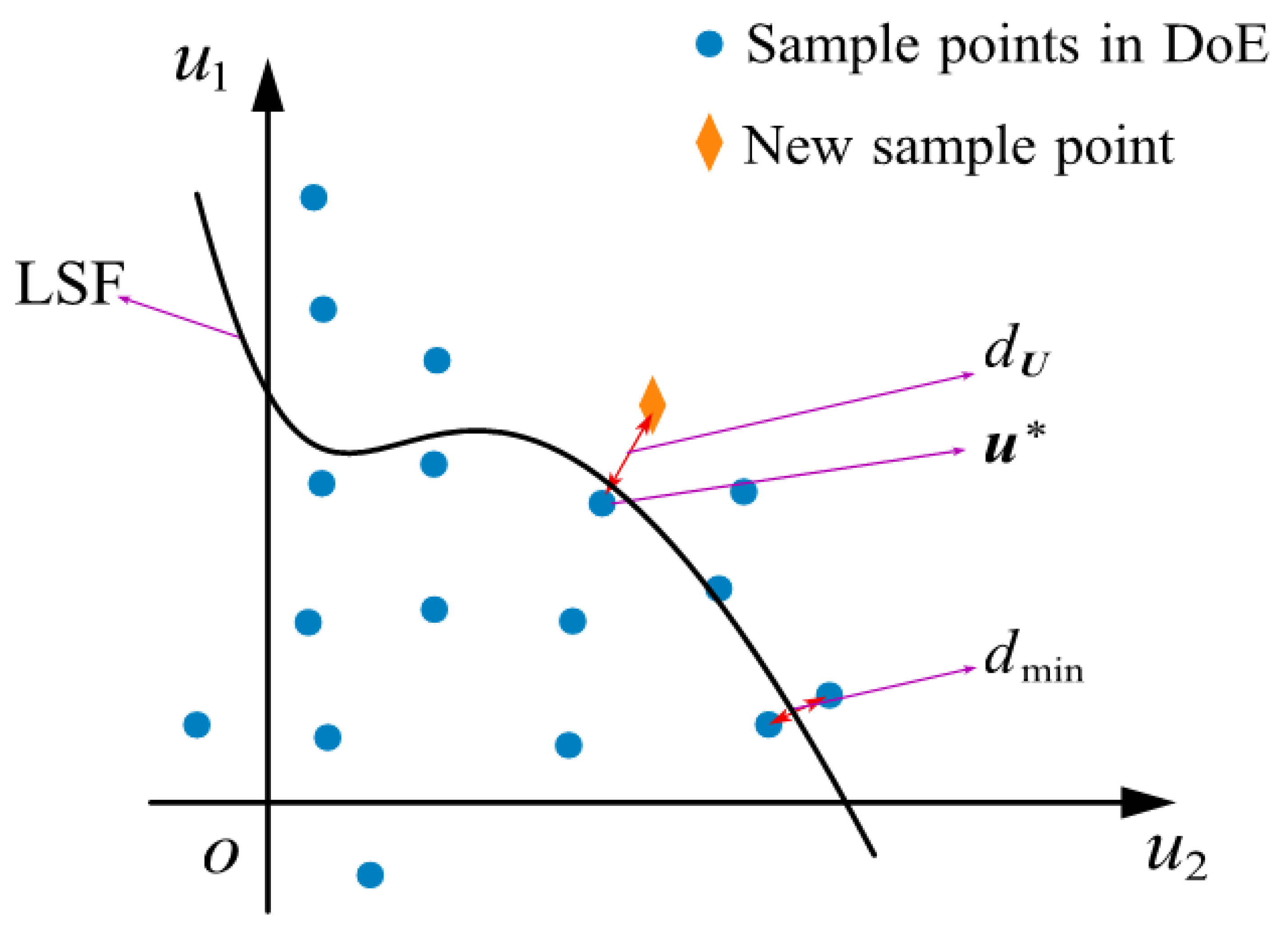
3.3. Construction of the Learning Function

To improve the efficiency and accuracy of the surrogate model, a learning function needs to be developed for sequential sampling in order to screen new sample points (here, the new sample points are selected from the Monte Carlo sample pool). Firstly, to maximize the contribution of the new sample points to the fitting accuracy of the meta model, the new sample points need to be close enough to the LSF. Secondly, to avoid clustering problems caused by samples being too close, new sample points need to maintain a sufficient distance from existing samples. So, the sample points are transformed by $\mathrm{U}=\mathrm{T}\left(\mathrm{X}\right)$ from the original space to a U-space with a standard normal random variable u (usually, Nataf or Rosenblatt transformations are used) [26]. The probability of sampling points in U-space is directly related to their Euclidean distance to the spatial origin, which has the advantage of avoiding the impact on distance caused by the order of magnitude differences among the components in the samples. To avoid clustering problems, a penalty function $d_{pen}\left(\mathrm{u}\right)$ is used to control the distance among sample points [24].

$$d_{pen}\left(\mathrm{u}\right):={\displaystyle \frac{d_U}{d_{min}}}={\displaystyle \frac{norm(\mathrm{u}-{\mathrm{u}}^{*})}{min\left(norm({\mathrm{u}}_i-{\mathrm{u}}_j)\right)}},i,j=1,2,\dots ,n_{DoE}\mathrm{and}i\ne j$$

(15)

whereby u is X that transforms from the original space to the U space; $d_{min}$ is the minimum distance among sample points of DoE in U space; ${\mathrm{u}}^{*}$ is the sample point in DoE that is closest to the new sample point in U space. So, $d_U$ is the distance between the new sample point and ${\mathrm{u}}^{*}$. $norm(·)$ means the two-norm function. ${\mathrm{u}}_i$ and ${\mathrm{u}}_j$ are the i-th and j-th sample points in DoE, respectively.

Figure 2 is a schematic diagram of $d_U$, $d_{min}$ and ${\mathrm{u}}^{*}$. Penalty functions can support the learning function to select new sample points that are further away from DoE, in which the normalization of input variables must be performed to ensure effectiveness of $d_{pen}\left(\mathrm{u}\right)$.

Based on the above requirements, an active learning function $LF\left(\mathrm{u}\right)$ is proposed by combining penalty functions $d_{pen}\left(\mathrm{u}\right)$

$$LF\left(\mathrm{u}\right)=\left({\left.{\displaystyle \frac{1}{|{\widehat{G}}_{mean}|+1}}\right)}^{\alpha UCF\left(\mathrm{u}\right)}\right.d_{pen}\left(\mathrm{u}\right)$$

(16)

whereby $UCF\left(\mathrm{u}\right)$ is a uncertain function to characterize the local uncertainty of approximate models at candidate sample points. $\alpha$ is an adjustment coefficient used for regulating function $UCF\left(\mathrm{u}\right)$, and $UCF\left(\mathrm{u}\right)$ can be expressed as

$$UCF\left(\mathrm{u}\right)=1+{\sigma }_w$$

(17)

With the help of $UCF\left(\mathrm{u}\right)$, the learning function will be more inclined to select candidate sampling points with greater uncertainty. According to the learning function given by Equation (16), the point with the greatest value of the learning function will be selected as the new sample point to be added to DoE. Hence, when the penalty function $d_{pen}\left(\mathrm{u}\right)>1$, it is a reward to $LF\left(\mathrm{u}\right)$; else, it is a punishment. Finding the sampling point with the maximum value of $LF\left(\mathrm{u}\right)$ is an optimization problem for which the MCS method is used to solve the optimization problem in this work. The MCS method can significantly reduce computational complexity, while optimization algorithms, such as genetic algorithms [28] or particle swarm optimization [29], require searching the variable space and may result in finding better sample points, but optimization algorithms also require more computational resources.

3.4. Failure Probability

According to Section 3.3, the update of the RBF model is iteratively performed as new sample points are continuously added to the learning function. When the iteration stops, the RBF proxy model can achieve the expected accuracy. Assuming k iterations are performed, the failure probability ${\widehat{P}}_f^k$ can be evaluated as

$${\widehat{P}}_f^k={\displaystyle \frac{1}{n_{mcs}}}\sum _{i=1}^{n_{mcs}}I(\widehat{g}\left(\mathrm{u}\right)<0)$$

(18)

whereby $n_{mcs}$ is the number of given Monte Carlo (MC) sample points, and $I(·)$ is the indicator function. When the internal indicators of the indicator function are satisfied, $I(·)=1$; otherwise, $I(·)=0$. Furthermore, the relative error of the predicted failure probability can be used as a stopping criterion to evaluate the iteration [26]

$${\displaystyle \frac{|\Delta {\widehat{P}}_f^k|}{{\widehat{P}}_f^k}}<\epsilon$$

(19)

whereby ${\widehat{P}}_f^{k-1}$ is the failure probability of the $(k-1)$ th iteration, and $\Delta {\widehat{P}}_f^k={\widehat{P}}_f^k-{\widehat{P}}_f^{k-1}$; $\epsilon$ is a user-defined termination number of the iteration. The coefficient of variation ($COV$) of MCS will also be an important indicator to evaluate the stopping of iterations [30], and $COV$ is defined as

$$COV:=\sqrt{{\displaystyle \frac{1-{\widehat{p}}_f}{n_{mcs}{\widehat{p}}_f}}}$$

(20)

whereby $n_{mcs}$ is the number of sample points in the MC population, ${\epsilon }_{cov}$ is the discriminant number of $COV$, and a reference value of ${\epsilon }_{cov}$ is 0.05 in Ref. [30].

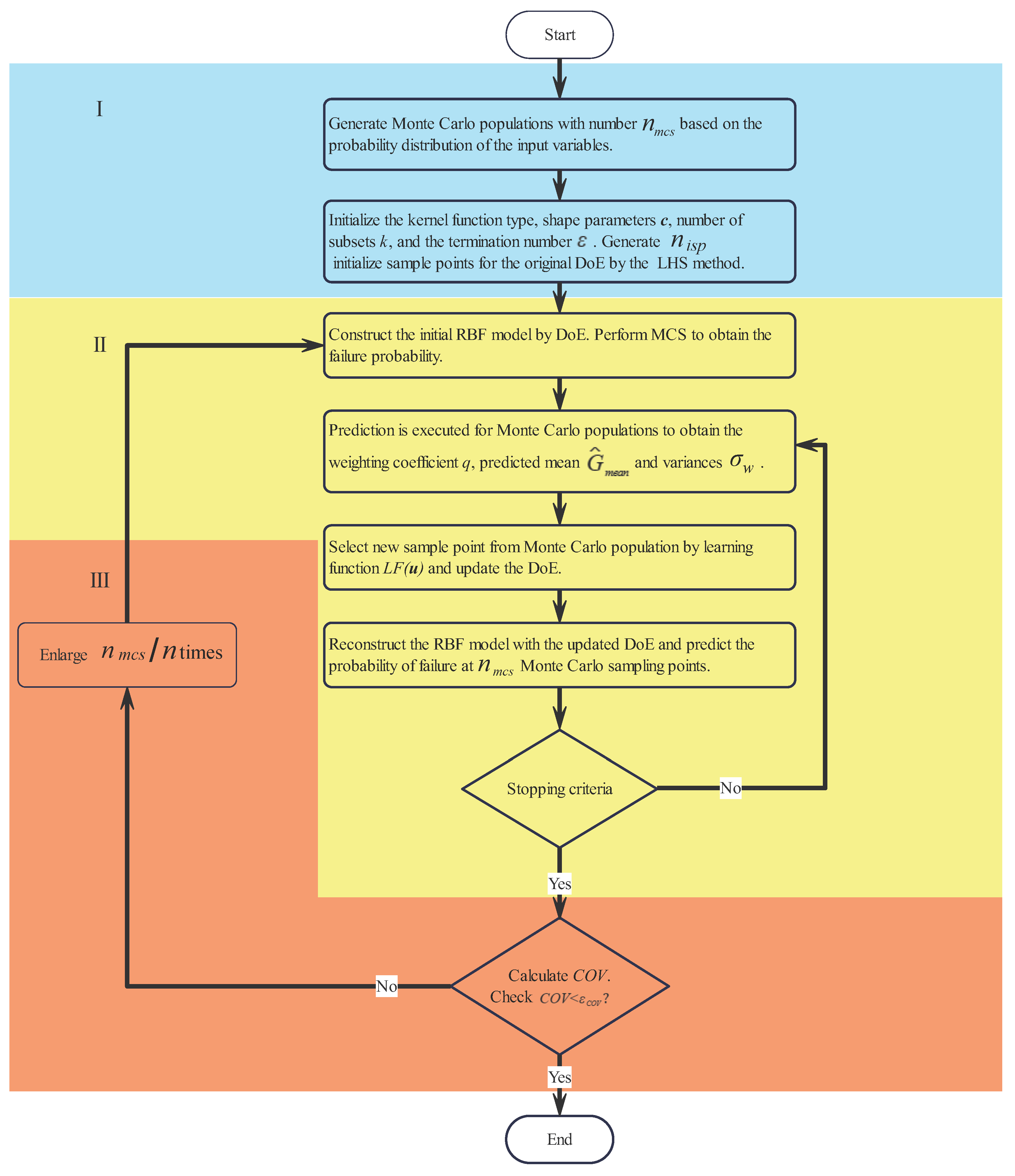
3.5. Main Steps of Active Learning Process

The flowchart of the ${\mathrm{P}}_{\sigma }$RBF-MCS method proposed is shown in Figure 3, and its steps are as follows.

• Step 1: Generating an MC population with a size of $n_{mcs}$ based on the probability distribution of the input variables.
• Step 2: Initializing the kernel function type, shape parameters c, subset number k, and termination number $\epsilon$ of the RBF model, and generating P initial sample points that form the initial DoE by using the Limit State Function (LSF) method.
• Step 3: Constructing the initial RBF model through initial DoE, and then obtaining the failure probability by MCS.
• Step 4: Predicting MC populations to obtain weighted coefficients $q_i$, predicted mean ${\widehat{G}}_{mean}$, and predicted mean variance ${\sigma }_w$.
• Step 5: Selecting new sample points from MC population by using learning functions $LF\left(\mathrm{u}\right)$ and updating DoE.
• Step 6: Reconstructing the RBF model based on Equation (1) by using the updated DoE, and predicting the failure probabilities of $n_{mcs}$ MC sampling points.
• Step 7: Executing stop criteria judgment. If satisfied, going to the next step of judgment, otherwise, returning to step 4 to continue iterating.
• Step 8: Calculating $COV$ and determining if it is less than ${\epsilon }_{cov}$. If satisfied, ending iteration; otherwise, expanding $n_{mcs}$ by 10 times and returning to step 3.

3.6. Implementation Details

The proposed P$\sigma$RBF-MCS framework was implemented using a combination of numerical and programming tools. Specifically, all surrogate modeling components, including Latin Hypercube Sampling (LHS), RBF model training, PRESS error computation, predicted variance evaluation, and the active learning function, were coded in MATLAB R2023a. Matrix operations, Euclidean distance computations, and sequential sample selection were performed using built-in numerical functions and custom optimization routines. The Monte Carlo sampling population and failure probability evaluations were also conducted within MATLAB.

The finite element simulation of interface oxidation failure, including thermal–stress coupling and crack propagation analysis based on a phase-field method, was carried out using COMSOL^® Multiphysics 6.0 [31]. This platform enabled the modeling of multi-layered TBC structures under thermal exposure, with geometry, meshing, and boundary conditions as described in Section 5.1.

The integration between the simulation data (from COMSOL) and the surrogate-based reliability framework (in MATLAB) was achieved via exported datasets, which were then used to calibrate the performance function $g\left(X\right)$ and update the DoE for reliability prediction.

Figure 3. Flowchart of ${\mathrm{P}}_{\sigma }$RBF-MCS method. The question mark "?" denotes a conditional check evaluating either convergence ("Stopping criteria") or whether the failure probability’s COV is below the threshold ${\epsilon }_{cov}$.

Figure 3. Flowchart of ${\mathrm{P}}_{\sigma }$RBF-MCS method. The question mark "?" denotes a conditional check evaluating either convergence ("Stopping criteria") or whether the failure probability’s COV is below the threshold ${\epsilon }_{cov}$.

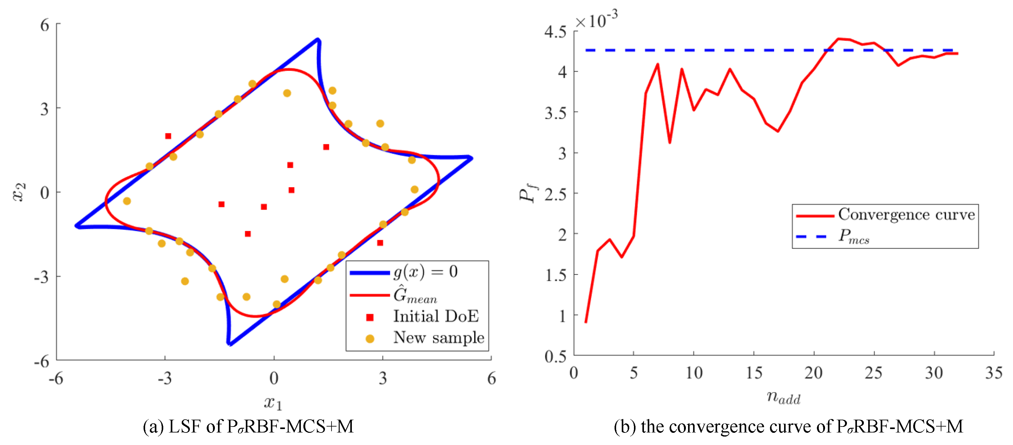
4. Example Verification

In this section, the feasibility and effectiveness of the ${\mathrm{P}}_{\sigma }$RBF-MCS method is verified through a two-dimensional problem of a four-branch series system, and the parameters that affect the performance, such as kernel function type, the number of multiple-prediction subsets k, and the adjustment coefficient $\alpha$, are also investigated. In the example, the number of function, called $n_{call}$, is used as the indicator of the efficiency for different methods. The number that a function is called is defined as the sum of the initial number of sample points $n_{isp}$ and the number of newly added points $n_{add}$:

$$n_{call}=n_{isp}+n_{add}$$

(21)

The accuracy index $e_{pe}$ is defined as

$$e_{pe}={\displaystyle \frac{\left|{\widehat{P}}_f-P_{mcs}\right|}{P_{mcs}}}$$

(22)

whereby $P_{mcs}$ and ${\widehat{P}}_f$ are the failure probabilities obtained from MCS and ${\mathrm{P}}_{\sigma }$RBF-MCS, respectively. A four-branch nonlinear series system is used for validation of the proposed model. The input random variables of the system, $x_1$ and $x_2$, are independent of each other and follow a standard normal distribution. The function of the system is [24]

$$g(x_1,x_2)=min\left\{\begin{array}{c}3+0.1\times {(x_1-x_2)}^2-(x_1+x_2)/\sqrt{2}\hfill \\ 3+0.1\times {(x_1-x_2)}^2+(x_1+x_2)/\sqrt{2}\hfill \\ (x_1-x_2)+6/\sqrt{2}\hfill \\ -(x_1-x_2)+6/\sqrt{2}\hfill \end{array}\right.$$

(23)

Here, $n_{mcs}$ is taken as ${10}^6$, the termination number $\epsilon$ is ${10}^{-5}$, and the initial training sample point P in DoE is 8. Firstly, the impact of different kernel functions on the ${\mathrm{P}}_{\sigma }$RBF-MCS method is discussed and the results are shown in Figure 4, Figure 5 and Figure 6, where Gaussian, multi-quadratic, and Inverse Multi-quadratic (IM) kernel functions are used in Figure 4, Figure 5 and Figure 6, respectively. From Figure 4, Figure 5 and Figure 6, the areas enclosed by LSF of ${\mathrm{P}}_{\sigma }$RBF-MCS+G and ${\mathrm{P}}_{\sigma }$RBF-MCS+IM are significantly larger than the actual safety zone, which is also the reason why the predicted failure probabilities of ${\mathrm{P}}_{\sigma }$RBF-MCS with these two kernel functions are smaller compared to MCS, and their convergence curves fluctuate more significantly. The fitting and prediction accuracy of the LSF for ${\mathrm{P}}_{\sigma }$RBF-MCS+M is clearly better than the other two methods, as shown in Figure 5, so the following discussion will be carried out on the case of ${\mathrm{P}}_{\sigma }$RBF-MCS+M.

Firstly, the impact of different subset sizes, $k_f=[3,4,5]$, on the proposed method are discussed and the results are listed in Table 2. With the increase in the number of subsets, the efficiency and accuracy of the ${\mathrm{P}}_{\sigma }$RBF-MCS method increase as well, which is due to the increase in uncertainty of the candidate sample points caused by the increase in $k_f$. However, due to the limitation of the initial sample points [25], $k_f$ cannot be increased continuously. When $k_f=5$ and $\alpha =[0.2,0.4,0.6,0.8,1]$, the impact of adjusting parameter $\alpha$ is evaluated as shown in Table 2.

Figure 5. LSF and convergence curve of the ${\mathrm{P}}_{\sigma }$RBF-MCS+M model.

Figure 5. LSF and convergence curve of the ${\mathrm{P}}_{\sigma }$RBF-MCS+M model.

Figure 6. LSF and convergence curve of the ${\mathrm{P}}_{\sigma }$RBF-MCS+IM model.

Figure 6. LSF and convergence curve of the ${\mathrm{P}}_{\sigma }$RBF-MCS+IM model.

Table 2. Average result of $P_{\sigma }$RBF for 10 runs.

Results of MCS or References	Method	${\mathit{n}}_{\mathbf{call}}$	${\mathit{P}}_{\mathit{f}}$ (%)	${\mathit{e}}_{\mathit{pe}}$ (%)
	MCS	${10}^6$	0.4324	/
Reference [24]	ARBFM-MCS	60.1	0.4466	1.13
Reference [24]	CVRBF-MCS ($\alpha =0$)	65.4	0.4480	1.44
Reference [32]	RBF-GA	33.3	0.4367	1.10
Reference [26]	MCRBF-MCS	36.3	0.4479	1.43
$P_{\sigma }$RBF method	$P_{\sigma }$RBF+IM ($k_f=5$, $\alpha =1$)	73.4	0.4473	3.44
	$P_{\sigma }$RBF+G ($k_f=5$, $\alpha =1$)	35.6	0.4382	1.36
	($k_f=3$, $\alpha =1$)	41.8	0.4383	1.02
	($k_f=4$, $\alpha =1$)	42.3	0.4374	0.96
	$P_{\sigma }$RBF+M ($k_f=5$, $\alpha =0.2$)	58.9	0.4197	2.94
	($k_f=5$, $\alpha =0.4$)	64.2	0.4267	1.32
	($k_f=5$, $\alpha =0.6$)	38.2	0.4251	1.68
	($k_f=5$, $\alpha =0.8$)	43.3	0.4300	1.26
	($k_f=5$, $\alpha =1$)	40.8	0.4365	0.94

Table 2. Average result of $P_{\sigma }$RBF for 10 runs.

Results of MCS or References	Method	${\mathit{n}}_{\mathbf{call}}$	${\mathit{P}}_{\mathit{f}}$ (%)	${\mathit{e}}_{\mathit{pe}}$ (%)
	MCS	${10}^6$	0.4324	/
Reference [24]	ARBFM-MCS	60.1	0.4466	1.13
Reference [24]	CVRBF-MCS ($\alpha =0$)	65.4	0.4480	1.44
Reference [32]	RBF-GA	33.3	0.4367	1.10
Reference [26]	MCRBF-MCS	36.3	0.4479	1.43
$P_{\sigma }$RBF method	$P_{\sigma }$RBF+IM ($k_f=5$, $\alpha =1$)	73.4	0.4473	3.44
	$P_{\sigma }$RBF+G ($k_f=5$, $\alpha =1$)	35.6	0.4382	1.36
	($k_f=3$, $\alpha =1$)	41.8	0.4383	1.02
	($k_f=4$, $\alpha =1$)	42.3	0.4374	0.96
	$P_{\sigma }$RBF+M ($k_f=5$, $\alpha =0.2$)	58.9	0.4197	2.94
	($k_f=5$, $\alpha =0.4$)	64.2	0.4267	1.32
	($k_f=5$, $\alpha =0.6$)	38.2	0.4251	1.68
	($k_f=5$, $\alpha =0.8$)	43.3	0.4300	1.26
	($k_f=5$, $\alpha =1$)	40.8	0.4365	0.94

The number of calling the LSF is significantly high when $\alpha$ is small, since a smaller $\alpha$ will reduce the impact of local uncertainty of the RBF approximation model at candidate sample points. The prediction error of the ${\mathrm{P}}_{\sigma }$RBF-MCS method is the smallest in the case of $k_f=5$ and $\alpha =1$, and the accuracy is higher than other methods; that is, $e_{pe}=0.94\%$ at the same time. In terms of computational efficiency, the number of calling functions for the ${\mathrm{P}}_{\sigma }$RBF-MCS method is only lower than that of the RBF-GA method and MCRBF method. In a word, the results in Table 2 indicate that the proposed method focuses more on improving the accuracy.

5. Reliability Assessment of TBC Interface Oxidation Failure

The failure process of the TBC system is quite complex, and the results of its failure behavior largely rely on numerical methods. In this work, numerical simulations of interface oxidation crack propagation are conducted based on the work of reference [33].

$$\left\{\begin{array}{c}\dot{C}-\nabla ·(D\nabla C)=-M\zeta (1-n)C\hfill \\ \dot{n}=\zeta (1-n)C\hfill \\ \nabla ·\sigma =\rho \dot{v}\hfill \\ \rho c_p\dot{\theta }+\nabla ·J=\gamma \hfill \\ G_c\left(d-l_0^2{\nabla }^{2}d\right)=2(1-d){\zeta }_l{l}_0\hfill \end{array}\right.$$

(24)

where c is the distribution of oxygen concentration, D is the oxygen diffusion coefficient, M represents the molar concentration of oxygen in ${\mathrm{Al}}_2{\mathrm{O}}_3$, $\zeta$ denotes the reaction rate control coefficient, n is the mole fraction of the TGO, J is the boundary condition for a given heat flux, $\rho$ and $\ddot{v}$ represent density and acceleration, $l_0$, respectively, and width of the crack, d is similar to the material stiffness, and $G_c$ represents the critical energy release rate of the material.

Furthermore, a failure criterion is constructed based on numerical simulations to validate the applicability of the proposed method in TBC problems.

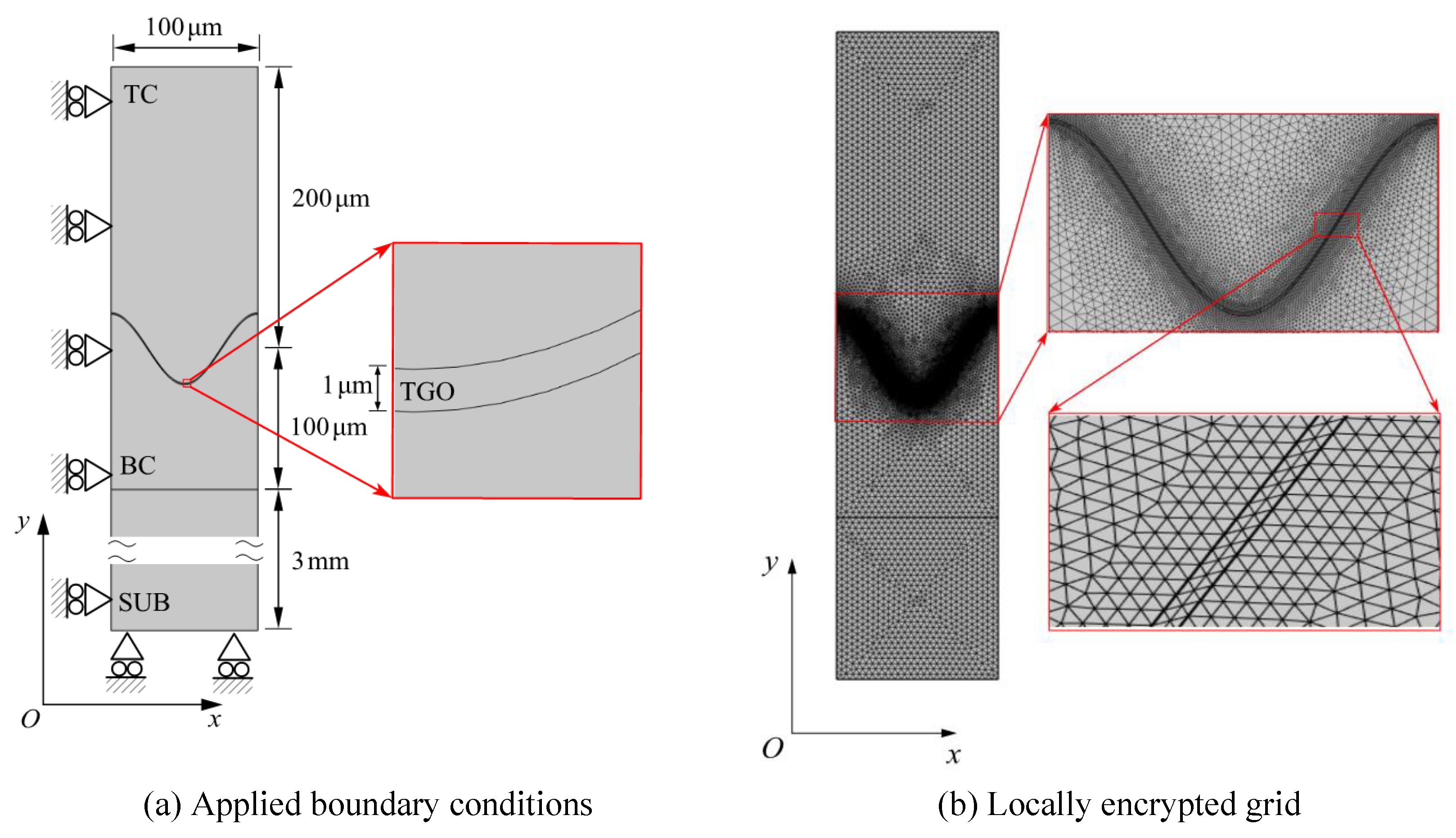
5.1. Finite Element Model and Boundary Conditions

All numerical simulations were conducted using COMSOL Multiphysics 6.0 on a high-performance workstation equipped with an Intel^® Core™ i7 processor (3.6 GHz, 16 cores), 64 GB RAM, and an NVIDIA^® RTX 3080 GPU. According to the company’s official website, Intel’s Chinese manufacturing facilities are located in Shanghai and Chengdu. This setup provided the computational power necessary for coupled thermo-mechanical and phase-field fracture modeling. The surrogate modeling and reliability analysis, including Monte Carlo sampling, radial basis function construction, and active learning functions, were implemented using custom scripts developed in MATLAB R2023a. These tools and computational resources ensured accurate resolution of the crack propagation behavior and efficient probabilistic analysis under varying input conditions.

The finite element model of the thermal barrier coating used for numerical simulation is shown in Figure 7 and the material properties of each TBC layer used in the simulation are listed in Table 3, with a ceramic layer thickness of 200 $\mathsf{\mu }$m, an oxide layer thickness of 1 $\mathsf{\mu }$m, a bonding layer thickness of 100 $\mathsf{\mu }$m, and a substrate thickness of 3 mm. It should be noted that there is no oxide layer present ideally when TBC is just prepared. However, in the actual preparation process, TBC lies in a high-temperature environment, which results in the formation of an oxide layer on the newly prepared TBC, and the thickness of the oxide layer is set to 1 $\mathsf{\mu }$m. Meanwhile, considering the actual interface morphology characteristics of APS TBC, the interfaces between the ceramic layer and the oxide layer, as well as between the oxide layer and the adhesive layer, are assumed to be an idealized cosine curve [34].

As shown in Figure 7, the horizontal degrees of freedom of the left edge and the vertical degrees of freedom of the lower edge of the model are fixed; that is, $u{|}_{x=0}=0$, $v{|}_{y=0}=0$. The right edge is set as a periodic boundary, $u{|}_{x=0}=u{|}_{x=100}$, and the vertical surface force of the upper edge is zero [33]. For the temperature field, the TBC system first undergoes an isothermal period of 800 h at 1150 °C, and then cools from 1150 °C to 20 °C within 0.5 h [35]. Due to the porous material used in the topmost ceramic layer, the diffusion rate of oxygen in the ceramic layer is much higher than that in the oxide layer and bonding layer, and no oxidation reaction occurs in the ceramic layer. Therefore, in order to reduce simulation calculation time, the oxygen concentrations at the interface between the ceramic layer and the oxide layer, as well as the interface between the bonding layer and the substrate, are set as the boundary conditions, as listed in

Table 4. Material properties related to the growth of the oxide layer.

Material Properties	Values
Oxygen diffusion coefficient in bonding layer $D^{\mathrm{BC}}$ (${\mathrm{m}}^2$/s)	2 × ${10}^{-12}$
Oxygen diffusion coefficient in oxide layer $D^{\mathrm{TGO}}$ (${\mathrm{m}}^2$/s)	2 × ${10}^{-12}$
Oxygen reaction rate $\zeta$ (${\mathrm{m}}^3$ ${\mathrm{mol}}^{-1}$ $s^{-1}$)	1 × ${10}^{-3}$
Molar concentration of oxygen M (mol ${\mathrm{m}}^{-3}$)	1.11 × ${10}^5$

.

Table 3. Material parameters of each layer of TBC used in numerical simulation [33,36].

	Ceramic Layer	Oxide Layer	Bonding Layer	Substrate
Young’s modulus E (GPa)	35	375	120	160
Poisson’s ratio v	0.1	0.25	0.32	0.33
density $\rho$ (kg/${\mathrm{m}}^3$)	5650	3978	8100	8100
tensile strength $f_t$ (GPa)	0.2	0.38	0.5	/
Fracture energy $\gamma$ (J/${\mathrm{m}}^2$)	61	49	47	/
Coefficient of thermal expansion $\alpha$ (${\mathrm{K}}^{-1}$)	9.8 × ${10}^{-6}$	9.2 × ${10}^{-6}$	1.4 × ${10}^{-7}$	1.5 × ${10}^{-7}$
Critical energy release rate $G_c$ (N/mm)	50	40	2700	2700
Thermal conductivity coefficient $\lambda$ (${\mathrm{Wm}}^{-1}$${\mathrm{K}}^{-1}$)	1.16	4.4	14.5	26

Table 3. Material parameters of each layer of TBC used in numerical simulation [33,36].

	Ceramic Layer	Oxide Layer	Bonding Layer	Substrate
Young’s modulus E (GPa)	35	375	120	160
Poisson’s ratio v	0.1	0.25	0.32	0.33
density $\rho$ (kg/${\mathrm{m}}^3$)	5650	3978	8100	8100
tensile strength $f_t$ (GPa)	0.2	0.38	0.5	/
Fracture energy $\gamma$ (J/${\mathrm{m}}^2$)	61	49	47	/
Coefficient of thermal expansion $\alpha$ (${\mathrm{K}}^{-1}$)	9.8 × ${10}^{-6}$	9.2 × ${10}^{-6}$	1.4 × ${10}^{-7}$	1.5 × ${10}^{-7}$
Critical energy release rate $G_c$ (N/mm)	50	40	2700	2700
Thermal conductivity coefficient $\lambda$ (${\mathrm{Wm}}^{-1}$${\mathrm{K}}^{-1}$)	1.16	4.4	14.5	26

At the same time, to simplify the model, it is assumed that the diffusion rate of oxygen in the oxide layer and bonding layer is the same, and the diffusion rate and reaction rate of oxygen in the oxide layer and bonding layer are increased. The parameters related to the growth of the oxide layer [37,38] are also given in Table 4.

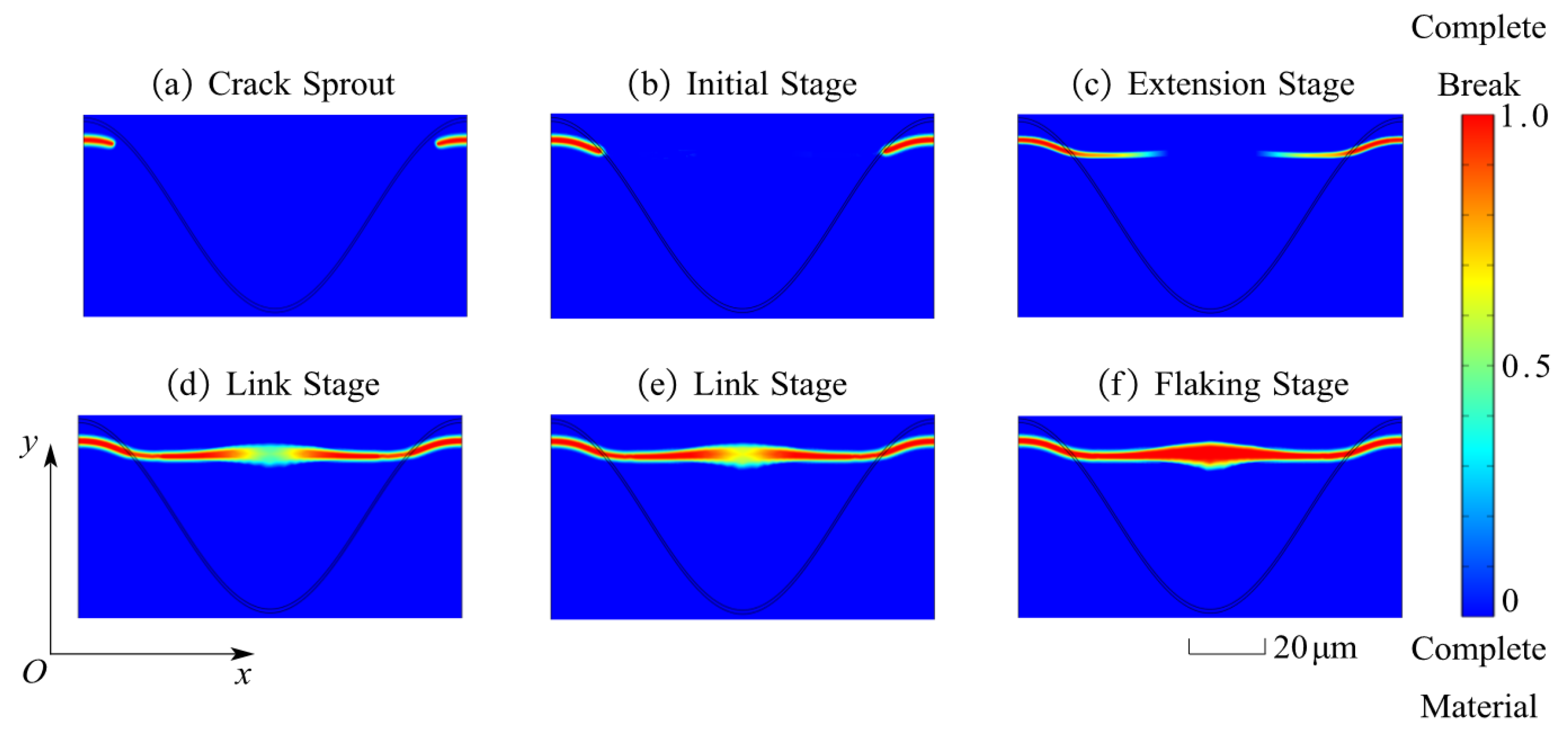
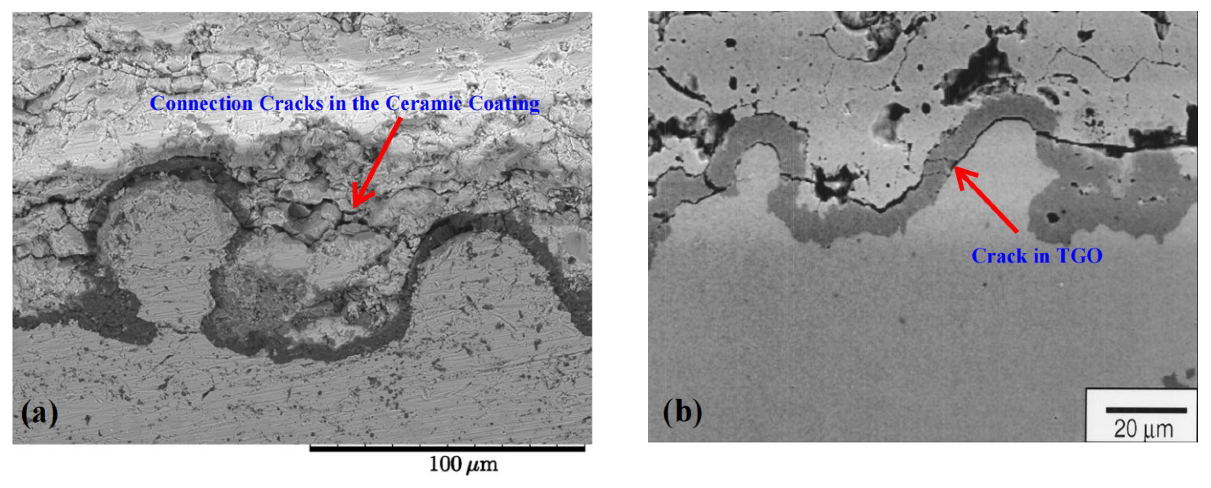
5.2. Numerical Simulation Results

Based on the boundary conditions and material parameters mentioned above, numerical simulations were conducted when ratios of amplitude to wavelength (A/L) were 1/4 and 1/8, respectively. The results are shown in Figure 8 and Figure 9. In Figure 8, the propagation behavior of cracks from initiation to connection is displayed, which leads to coating peeling. In Figure 8a,b, the cracks first appear in the oxide layer near the ceramic layer interface and gradually grow to the ceramic layer interface. In Figure 8c,d, the crack continues to grow horizontally after passing through the interface. In Figure 8e,f, cracks are generated at adjacent peaks at both ends connected within the ceramic layer, leading to the delamination of TBC. The simulation results are consistent with TBC interface oxidation failure during the actual service process [39], which can be used for the construction of failure criteria.

In Figure 9, the propagation behavior of cracks from initiation to connection, resulting in coating peeling when A/L = 1/8, is illustrated. From Figure 9a, it can be seen that in the initial stage of crack initiation, cracks also occur in the oxide layer. However, the difference is that in the crack growth stages shown in Figure 9b,c, the crack does not pass through the ceramic layer interface, but grows along the oxide layer, and as shown in Figure 9d, the cracks at both ends connect at the valley, causing coating peeling.

Compared with the experimental observation results shown in Figure 10, it can be seen that the numerical simulation results are consistent with the crack propagation trend shown in the SEM image of the TBC after a period of service [39,40]. In Figure 10a, when A/L = 1/4, cracks first originate from the oxide layer region near the ceramic layer and propagate to the ceramic layer, ultimately connecting within the ceramic layer. In Figure 10b, when A/L = 1/8, cracks are generated in the oxide layer area near the adhesive layer, and then grow along and pass through the oxide layer, connecting in the area near the ceramic layer. The comparison of the above results indicates that a failure criterion for TBC interface oxidation can be established and reliability analysis can be conducted based on the numerical simulation.

It should be noted that the experimental results shown in Figure 10 are adapted from references [39,40], where (APS) TBC samples were prepared with a multi-layer structure consisting of a zirconia-based top coat, a bond coat, and a superalloy substrate. The ceramic layer was approximately 200 $\mathsf{\mu }$m thick with a rough cosine-profiled interface. Mechanical testing indicated a tensile strength of 0.2–0.4 GPa for the ceramic and oxide layers, consistent with the values used in our simulations. The SEM images revealed two distinct failure paths depending on the A/L ratio: crack propagation into the ceramic layer for A/L = 1/4, and interfacial delamination along the oxide layer for A/L = 1/8.

The simulation results captured these trends well: under identical A/L configurations, our finite element model showed crack initiation near the ceramic/oxide interface and subsequent coalescence in the same regions observed experimentally. This confirms the capability of the model to predict failure modes and interface degradation patterns under realistic thermal loading conditions.

While the SEM images presented in Figure 10 qualitatively validate the crack propagation trends observed in the simulation, direct cross-sectional measurements of oxidation penetration depth were not performed, as the images were sourced from prior literature [39,40]. Incorporating such measurements in future experimental campaigns would provide valuable quantitative data to further calibrate and validate the numerical model, particularly in establishing failure thresholds associated with oxide growth.

It is acknowledged that thermal exposure can induce phase transformations in ceramic and metallic layers, potentially influencing crack propagation and failure mechanisms. Although this study focused on numerical modeling and did not include experimental phase analysis, techniques such as X-ray diffraction (XRD) would be valuable in future work to detect possible crystallographic changes resulting from thermal cycling or oxidation processes. Such experimental insights could further refine the failure criteria and support more accurate prediction of TBC degradation.

5.3. Construction of Failure Criteria

Based on the above numerical model, an implicit failure criterion for TBC interface oxidation can be further constructed as follows:

$$g\left(X_i\right)=1-S\left(X_i\right)$$

(25)

whereby $S\left(X_i\right)$ is a function used to determine whether the selected location has cracked, and $X_i$ represents material parameters and environmental loads related to TBC interface oxidation failure, such as Young’s modulus, thermal expansion coefficient, and fracture toughness. When $S\left(X_i\right)=1$, the material has undergone complete fracture and the performance function $g\left(X_i\right)=0$. Obviously, for the established failure criteria, evaluating the failure location is of great significance. According to the geometric model, boundary conditions, and simulation results of numerical simulation, cracks always initiate at both ends and connect in the middle position (whether in the ceramic layer or the oxide layer).

Therefore, the evaluation of the failure position is selected as the geometric model axis shown in Figure 11; that is, $x=50\mathsf{\mu }\mathrm{m}$, which can best reflect the cracking state of TBC. At this point, when $S\left(X_i\right)=1$, it represents both the fracture of the material and the connection of cracks (indicating the delamination failure of the TBC structure).

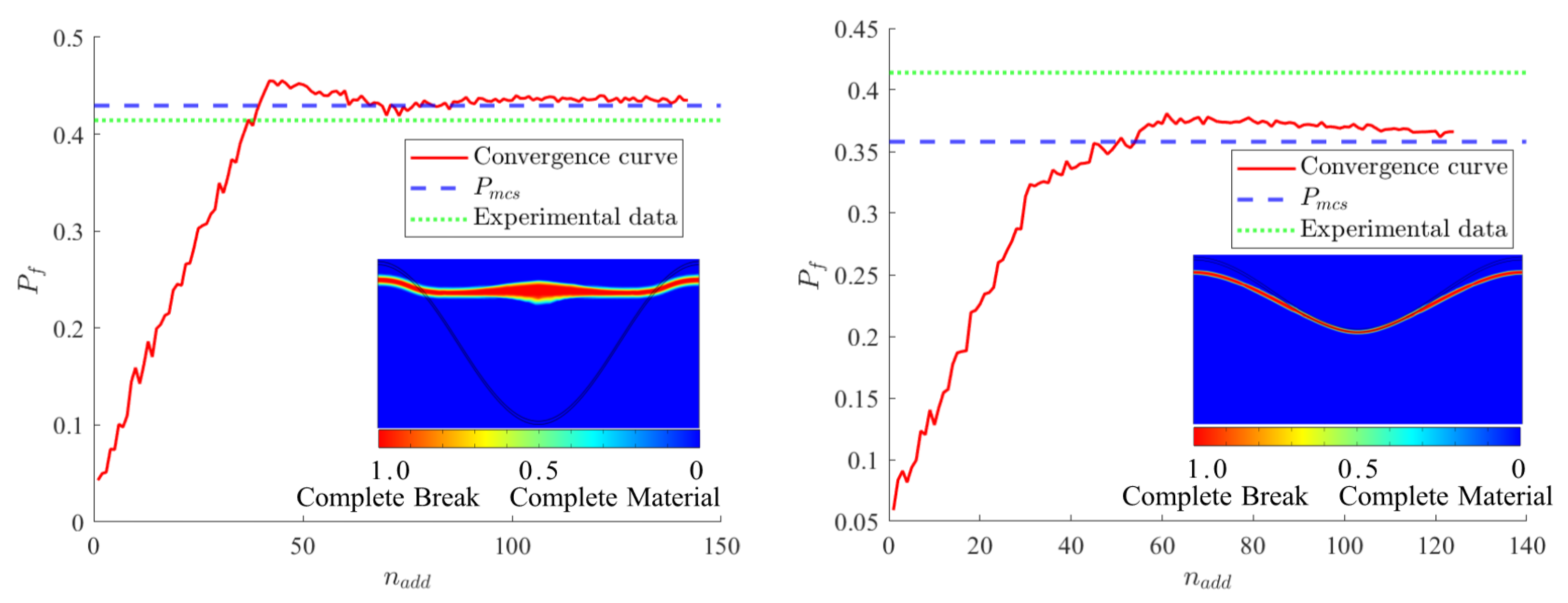
5.4. Reliability Calculation of TBC Interface Oxidation Failure Based on $P_{\sigma }$RBF-MCS Method

According to the implicit failure criterion in Equation (25), the reliability is analyzed based on the proposed $P_{\sigma }$RBF-MCS method. Firstly, the statistical characteristics of the random variable parameters $X_i$ in Equation (25) are analyzed. The random variables are listed in

Table 5. Numerical characteristics of random variables.

Random Variable	Distribution Type	Mean Value	Standard
Young’s modulus	$E_{tc}$ (GPa)	Normal distribution	380	100
	$E_{tgo}$ (GPa)	Normal distribution	120	30
Thermal expansion coefficient	${\alpha }_{tc}$ (${10}^{-6}$/K)	Normal distribution	9.2	0.37
	${\alpha }_{tgo}$ (${10}^{-6}$/K)	Normal distribution	9.8	0.39
Fracture energy	${\gamma }_{tc}$ (J/${\mathrm{m}}^2$)	Weibull distribution	60	6
	${\gamma }_{tgo}$ (J/${\mathrm{m}}^2$)	Weibull distribution	50	5
Temperature difference	$\Delta T$ (°C)	Normal distribution	1050	5

[41,42,43,44,45,46], and temperature difference $\Delta T$ between insulation temperature and ambient temperature of the ceramic layer and oxide layer is also random.

Whereby subscripts $tc$ and $tgo$ mean ceramic layer and oxide layer, respectively.

Here, the parameters of the $P_{\sigma }$RBF-MCS model are set as follows. The MC population size $n_{mcs}$ is $5\times {10}^3$, the initial sample population in DoE $n_{isp}$ is 12, the termination number $\epsilon$ is ${10}^{-4}$, the kernel function is multi-quadratic, the subset size k is 5, and adjustment coefficient $\alpha =1$. In addition to the results from $P_{\sigma }$RBF-MC method, the oxidation failure probabilities of the TBC interface obtained from the MC method and experiments [47] are also listed in

Table 6. Results of the reliability for TBC.

Method	Failure Probability ${\mathit{P}}_{\mathit{f}}$ (%)	Efficiency ${\mathit{N}}_{\mathbf{call}}$	Accuracy ${\mathit{e}}_{\mathit{pe}}$ (%)
Experiment [47]	41.4	/	/
MC ($A/L=1/4$)	42.9	5 × ${10}^3$	/
MC ($A/L=1/8$)	35.8	5 × ${10}^3$	/
$P_{\sigma }$RBF-MC ($A/L=1/4$)	43.7	143.3	1.92
$P_{\sigma }$RBF-MC ($A/L=1/8$)	36.6	126.4	2.23

.

The error between the failure probabilities obtained from the $P_{\sigma }$RBF-MCS model and the experimental data are 5.56% (A/L = 1/4) and 11.6% (A/L = 1/8), respectively. Compared with the results of the MC method, fewer functions are called with the $P_{\sigma }$RBF-MC method. In general, the reliability analysis based on the $P_{\sigma }$RBF-MCS model can effectively predict the failure probability of TBC interface oxidation failure and has higher efficiency.

From Figure 12, the experimental data [47], the failure probabilities from $P_{\sigma }$RBF-MCS model and MCS are illustrated, and the convergence failure probability from $P_{\sigma }$RBF-MCS model is very close to that of MCS and experiential data [47]. The predicted failure probability of the $P_{\sigma }$RBF-MCS model changes significantly in the early stages of active learning with fewer added points. This is when adding fewer points, each new point has a significant impact on the model. With the increase in the number of added points, the model tends to stabilize and eventually converges after satisfying the given termination number. The convergence curves of $P_{\sigma }$RBF-MCS model also reflect that the $P_{\sigma }$RBF-MCS method has a good convergence.

It is noted that while the training of the surrogate models in this work is based on numerical simulation data, the input parameters are carefully selected from experimentally validated sources in the literature to ensure physical fidelity. Furthermore, experimental SEM observations (Figure 10) are used to qualitatively support the failure mode assumptions. Future work may incorporate direct experimental datasets, such as mechanical testing results or in situ oxidation measurements, to further calibrate and validate the surrogate models.

6. Conclusions

In this work, the $P_{\sigma }$RBF-MCS method for analyzing the reliability of TBC interface oxidation is proposed. Firstly, an RBF initial model is constructed based on the initial DoE, and the initial model is updated by adding points later. The effectiveness of the proposed method ($P_{\sigma }$RBF-MCS) is verified via an example of four-branch series system. Finally, the reliability of TBC interface oxidation is evaluated based on the $P_{\sigma }$RBF-MCS method, and the following conclusions are obtained.

• When constructing multiple predictions with different numbers of DoE subsets $k_f$, the number of subsets $k_f$ has a significant impact on the sequential sampling used for updating the RBF model, since the quantity of $k_f$ affects the local uncertainty. Simultaneously adjusting the coefficient $\alpha$ also has an impact on the efficiency of the active learning function. When $\alpha$ is small, the influence of local uncertainty is reduced, which also reduces the differences among the candidate sample points. Therefore, for the $P_{\sigma }$RBF-MCS method, the performance is the best when $k_f=5$ and $\alpha =1$ in the example.
• The acceptable results under different subset numbers and adjustment coefficients can be obtained with the $P_{\sigma }$RBF-MCS method. The comparison with other methods in the literature can demonstrate the advantage of the proposed method in terms of accuracy.
• The accuracy and efficiency of reliability calculation for TBC oxidation failure problems can be improved via the proposed $P_{\sigma }$RBF-MCS method, and the results obtained are within the acceptable error range.

References

1. Khajezadeh, M.H.; Mohammadi, M.; Ghatee, M. Hot corrosion performance and electrochemical study of CoNiCrAlY/YSZ/YSZ-La2O3 multilayer thermal barrier coatings in the presence of molten salt. Mater. Chem. Phys. 2018, 220, 23–34. [Google Scholar] [CrossRef]
2. Clarke, D.; Levi, C. Materials design for the next generation thermal barrier coatings. Annu. Rev. Mater. Res. 2003, 33, 383–417. [Google Scholar] [CrossRef]
3. Liu, Y.; Liu, W.; Wang, W.; Zhang, W.; Yang, T.; Li, K.; Li, H.; Tang, Z.; Liu, C.; Zhang, C. Deposition characteristics, sintering and CMAS corrosion resistance, and mechanical properties of thermal barrier coatings by atmospheric plasma spraying. Surf. Coat. Technol. 2024, 482, 130623. [Google Scholar] [CrossRef]
4. Liu, L.; Liu, D.; Cai, H.; Mu, R.; Yang, W.; He, L. Failure of Electron Beam Physical Vapor Deposited Thermal Barrier Coatings System under Cyclic Thermo-Mechanical Loading with a Thermal Gradient. Coatings 2024, 14, 902. [Google Scholar] [CrossRef]
5. Zhang, H.; Chen, Y.; Li, L.; Yang, D.; Liu, X.; Huang, A.; Zhang, X.; Lu, J.; Zhao, X. Unraveling the CMAS corrosion mechanism of APS high-yttria-stabilized zirconia thermal barrier coatings. J. Eur. Ceram. Soc. 2024, 44, 5154–5165. [Google Scholar] [CrossRef]
6. Liu, Y.; Balakrishnan, G.; Hatnean, M.C.; Xiao, P.; Chen, Y. Anisotropic fracture in gadolinium zirconate single crystal: Micromechanical testing and modelling. Acta Mater. 2025, 289, 120944. [Google Scholar] [CrossRef]
7. Cheng, B.; Zhang, Y.M.; Yang, N.; Zhang, M.; Chen, L.; Yang, G.J.; Li, C.X.; Li, C.J. Sintering-induced delamination of thermal barrier coatings by gradient thermal cyclic test. J. Am. Ceram. Soc. 2017, 100, 1820–1830. [Google Scholar] [CrossRef]
8. Nordhorn, C.; Mücke, R.; Mack, D.E.; Vaßen, R. Probabilistic lifetime model for atmospherically plasma sprayed thermal barrier coating systems. Mech. Mater. 2016, 93, 199–208. [Google Scholar] [CrossRef]
9. Guo, J.W.; Yang, L.; Zhou, Y.C.; He, L.M.; Zhu, W.; Cai, C.Y.; Lu, C.S. Reliability assessment on interfacial failure of thermal barrier coatings. Acta Mech. Sin. 2016, 32, 915–924. [Google Scholar] [CrossRef]
10. Yan, Y.; Wang, X.; Li, Y. Structural reliability with credibility based on the non-probabilistic set-theoretic analysis. Aerosp. Sci. Technol. 2022, 127, 107730. [Google Scholar] [CrossRef]
11. Arndt, C.; Crusenberry, C.; Heng, B.; Butler, R.; TerMaath, S. Reduced-dimension surrogate modeling to characterize the damage tolerance of composite/metal structures. Modelling 2023, 4, 485–514. [Google Scholar] [CrossRef]
12. Luo, C.; Keshtegar, B.; Zhu, S.P.; Niu, X. EMCS-SVR: Hybrid efficient and accurate enhanced simulation approach coupled with adaptive SVR for structural reliability analysis. Comput. Methods Appl. Mech. Eng. 2022, 400, 115499. [Google Scholar] [CrossRef]
13. Alban, A.; Darji, H.A.; Imamura, A.; Nakayama, M.K. Efficient Monte Carlo methods for estimating failure probabilities. Reliab. Eng. Syst. Saf. 2017, 165, 376–394. [Google Scholar] [CrossRef]
14. Wang, J.; Li, C.; Xu, G.; Li, Y.; Kareem, A. Efficient structural reliability analysis based on adaptive Bayesian support vector regression. Comput. Methods Appl. Mech. Eng. 2021, 387, 114172. [Google Scholar] [CrossRef]
15. Teixeira, R.; Nogal, M.; O’Connor, A. Adaptive approaches in metamodel-based reliability analysis: A review. Struct. Saf. 2021, 89, 102019. [Google Scholar] [CrossRef]
16. Salazar-Rojas, T.; Cejudo-Ruiz, F.R.; Calvo-Brenes, G. Comparison between machine linear regression (MLR) and support vector machine (SVM) as model generators for heavy metal assessment captured in biomonitors and road dust. Environ. Pollut. 2022, 314, 120227. [Google Scholar] [CrossRef]
17. ALKannad, A.A.; Smadi, A.A.; AL-Makhlafi, M.; Yang, S.; Feng, Z. CrackVisionX: A Fine-Tuned Framework for Efficient Binary Concrete Crack Detection. IEEE Trans. Intell. Transp. Syst. 2025, 1–20. [Google Scholar] [CrossRef]
18. Deng, J.; Gu, D.; Li, X.; Yue, Z.Q. Structural reliability analysis for implicit performance functions using artificial neural network. Struct. Saf. 2005, 27, 25–48. [Google Scholar] [CrossRef]
19. Alkannad, A.A.; Al Smadi, A.; Yang, S.; Al-Smadi, M.K.; Al-Makhlafi, M.; Feng, Z.; Yin, Z. CrackVision: Effective Concrete Crack Detection with Deep Learning and Transfer Learning. IEEE Access 2025, 13, 29554–29576. [Google Scholar] [CrossRef]
20. Bai, G.; Fei, C. Distributed collaborative response surface method for mechanical dynamic assembly reliability design. Chin. J. Mech. Eng. 2013, 26, 1160–1168. [Google Scholar] [CrossRef]
21. Tamilarasan, A.; Rajamani, D. Metaheuristic Prediction Models for Kerf Deviation in Nd-YAG Laser Cutting of AlZnMgCu1.5 Alloy. Modelling 2025, 6, 17. [Google Scholar] [CrossRef]
22. Chen, Z.; Li, G.; He, J.; Yang, Z.; Wang, J. Adaptive structural reliability analysis method based on confidence interval squeezing. Reliab. Eng. Syst. Saf. 2022, 225, 108639. [Google Scholar] [CrossRef]
23. Singh, V.; Harursampath, D.; Dhawan, S.; Sahni, M.; Saxena, S.; Mallick, R. Physics-Informed Neural Network for Solving a One-Dimensional Solid Mechanics Problem. Modelling 2024, 5, 1532–1549. [Google Scholar] [CrossRef]
24. Shi, L.; Sun, B.; Ibrahim, D.S. An active learning reliability method with multiple kernel functions based on radial basis function. Struct. Multidiscip. Optim. 2019, 60, 211–229. [Google Scholar] [CrossRef]
25. Hong, L.; Li, H.; Peng, K. A combined radial basis function and adaptive sequential sampling method for structural reliability analysis. Appl. Math. Model. 2021, 90, 375–393. [Google Scholar] [CrossRef]
26. Du, W.; Ma, J.; Yue, P.; Gong, Y. An efficient reliability method with multiple shape parameters based on radial basis function. Appl. Sci. 2022, 12, 9689. [Google Scholar] [CrossRef]
27. Wei, Y.; Bai, G.; Song, L.K. A novel reliability analysis approach with collaborative active learning strategy-based augmented RBF metamodel. IEEE Access 2020, 8, 199603–199617. [Google Scholar] [CrossRef]
28. Ishaque, K.; Salam, Z.; Amjad, M.; Mekhilef, S. An improved particle swarm optimization (PSO)–based MPPT for PV with reduced steady-state oscillation. IEEE Trans. Power Electron. 2012, 27, 3627–3638. [Google Scholar] [CrossRef]
29. Dubourg, V.; Sudret, B.; Bourinet, J.M. Reliability-based design optimization using kriging surrogates and subset simulation. Struct. Multidiscip. Optim. 2011, 44, 673–690. [Google Scholar] [CrossRef]
30. Echard, B.; Gayton, N.; Lemaire, M. AK-MCS: An active learning reliability method combining Kriging and Monte Carlo simulation. Struct. Saf. 2011, 33, 145–154. [Google Scholar] [CrossRef]
31. COMSOL AB. AC/DC Module User’s Guide, Version 6.3 ed.; COMSOL AB: Stockholm, Sweden, 2024. [Google Scholar]
32. Jing, Z.; Chen, J.; Li, X. RBF-GA: An adaptive radial basis function metamodeling with genetic algorithm for structural reliability analysis. Reliab. Eng. Syst. Saf. 2019, 189, 42–57. [Google Scholar] [CrossRef]
33. Xiao, Y.; Liu, Z.; Peng, X.; Zhu, W.; Zhou, Y.; Yang, L. Spallation mechanism of thermal barrier coatings with real interface morphology considering growth and thermal stresses based on fracture phase field. Surf. Coat. Technol. 2023, 458, 129356. [Google Scholar] [CrossRef]
34. Zhou, Q.; Yang, L.; Luo, C.; Chen, F.; Zhou, Y.; Wei, Y. Thermal barrier coatings failure mechanism during the interfacial oxidation process under the interaction between interface by cohesive zone model and brittle fracture by phase-field. Int. J. Solids Struct. 2021, 214, 18–34. [Google Scholar] [CrossRef]
35. Shen, Q.; Yang, L.; Zhou, Y.; Wei, Y.; Zhu, W. Effects of growth stress in finite-deformation thermally grown oxide on failure mechanism of thermal barrier coatings. Mech. Mater. 2017, 114, 228–242. [Google Scholar] [CrossRef]
36. Xiao, Y.; Yang, L.; Zhu, W.; Zhou, Y.; Pi, Z.; Wei, Y. Delamination mechanism of thermal barrier coatings induced by thermal cycling and growth stresses. Eng. Fail. Anal. 2021, 121, 105202. [Google Scholar] [CrossRef]
37. Min, L.; Wang, Z.; Hu, X.; Zhao, D.; Sun, Z.; Zhang, P.; Yao, W.; Bui, T.Q. A chemo-thermo-mechanical coupled phase field framework for failure in thermal barrier coatings. Comput. Methods Appl. Mech. Eng. 2023, 411, 116044. [Google Scholar] [CrossRef]
38. Shen, Q.; Li, S.; Yang, L.; Zhou, Y.; Wei, Y.; Yuan, T. Coupled mechanical-oxidation modeling during oxidation of thermal barrier coatings. Comput. Mater. Sci. 2018, 154, 538–546. [Google Scholar] [CrossRef]
39. Al-Athel, K.; Loeffel, K.; Liu, H.; Anand, L. Modeling decohesion of a top-coat from a thermally-growing oxide in a thermal barrier coating. Surf. Coat. Technol. 2013, 222, 68–78. [Google Scholar] [CrossRef]
40. Rabiei, A.; Evans, A. Failure mechanisms associated with the thermally grown oxide in plasma-sprayed thermal barrier coatings. Acta Mater. 2000, 48, 3963–3976. [Google Scholar] [CrossRef]
41. Nie, J.Y.; Li, D.Q.; Cao, Z.J.; Zhou, B.; Zhang, A.J. Probabilistic characterization and simulation of realistic particle shape based on sphere harmonic representation and Nataf transformation. Powder Technol. 2020, 360, 209–220. [Google Scholar] [CrossRef]
42. Busso, E.P.; Wright, L.; Evans, H.; McCartney, L.; Saunders, S.; Osgerby, S.; Nunn, J. A physics-based life prediction methodology for thermal barrier coating systems. Acta Mater. 2007, 55, 1491–1503. [Google Scholar] [CrossRef]
43. Guo, S.; Kagawa, Y. Young’s moduli of zirconia top-coat and thermally grown oxide in a plasma-sprayed thermal barrier coating system. Scr. Mater. 2004, 50, 1401–1406. [Google Scholar] [CrossRef]
44. Jackson, R.D. The Effect of Bond Coat Oxidation on the Microstructure and Endurance of Two Thermal Barrier Coating Systems. Ph.D. Thesis, University of Birmingham, Birmingham, UK, 2010. [Google Scholar]
45. Sfar, K.; Aktaa, J.; Munz, D. Numerical investigation of residual stress fields and crack behavior in TBC systems. Mater. Sci. Eng. A 2002, 333, 351–360. [Google Scholar] [CrossRef]
46. Wan, J.; Zhou, M.; Yang, X.; Dai, C.; Zhang, Y.; Mao, W.; Lu, C. Fracture characteristics of freestanding 8 wt% Y2O3–ZrO2 coatings by single edge notched beam and Vickers indentation tests. Mater. Sci. Eng. A 2013, 581, 140–144. [Google Scholar] [CrossRef]
47. Wang, Z.; Wang, Z.; Zhang, T.; Guo, W.; Dai, H.; Ding, K. Reliability evaluation of thermal barrier coatings for engine combustion chambers based on Monte-Carlo simulation. Surf. Coat. Technol. 2022, 448, 128923. [Google Scholar] [CrossRef]
Figure 1. RBF model and distribution of prediction variance from −4 to 4.
Modelling 06 00061 g001
Figure 2. Distance control diagram.
Modelling 06 00061 g002
Figure 4. LSF and convergence curve of the P σ RBF-MCS+G model.
Modelling 06 00061 g004
Figure 7. Finite element geometric model diagram: (a) Applied boundary conditions, where the solid lines in the zoomed region represent the upper and lower interfaces of the thermally grown oxide (TGO) layer. (b) Locally encrypted mesh near the TGO region to ensure numerical accuracy [34].
Modelling 06 00061 g007
Figure 8. Numerical simulation results when A/L = 1/4.
Modelling 06 00061 g008
Figure 9. Numerical simulation results when A/L = 1/8.
Modelling 06 00061 g009
Figure 10. SEM of the oxidated TBC: (a) A/L = 1/4; (b) A/L = 1/8 [39,40].
Modelling 06 00061 g010
Figure 11. Schematic diagram for the evaluation of failure location in TBC.
Modelling 06 00061 g011
Figure 12. Convergence curve of P σ RBF-MCS.
Modelling 06 00061 g012