The Estimating Parameter and Number of Knots for Nonparametric Regression Methods in Modelling Time Series Data

Abstract

This research aims to explore and compare several nonparametric regression techniques, including smoothing splines, natural cubic splines, B-splines, and penalized spline methods. The focus is on estimating parameters and determining the optimal number of knots to forecast cyclic and nonlinear patterns, applying these methods to simulated and real-world datasets, such as Thailand’s coal import data. Cross-validation techniques are used to control and specify the number of knots, ensuring the curve fits the data points accurately. The study applies nonparametric regression to forecast time series data with cyclic patterns and nonlinear forms in the dependent variable, treating the independent variable as sequential data. Simulated data featuring cyclical patterns resembling economic cycles and nonlinear data with complex equations to capture variable interactions are used for experimentation. These simulations include variations in standard deviations and sample sizes. The evaluation criterion for the simulated data is the minimum average mean square error (MSE), which indicates the most efficient parameter estimation. For the real data, monthly coal import data from Thailand is used to estimate the parameters of the nonparametric regression model, with the MSE as the evaluation metric. The performance of these techniques is also assessed in forecasting future values, where the mean absolute percentage error (MAPE) is calculated. Among the methods, the natural cubic spline consistently yields the lowest average mean square error across all standard deviations and sample sizes in the simulated data. While the natural cubic spline excels in parameter estimation, B-splines show strong performance in forecasting future values.

1. Introduction

Regression analysis is a statistical method used to determine the relationship between an independent and a dependent variable, allowing for predictions of the dependent variable based on the independent one. However, there are cases where the assumptions underlying regression analysis may only apply to certain variables. An incorrect parametric model can lead to misleading interpretations [1,2]. Furthermore, there may be instances where a suitable parametric model does not exist. Nonparametric regression methods can be employed to address these challenges. These methods estimate parameters in situations where the data exhibit nonlinear relationships. Constructing a smoothing curve based on the available data is often called the smoothing method. This approach provides an alternative when traditional parametric models are either unsuitable or the regression analysis assumptions are not satisfied.

Nonparametric regression offers several advantages, making it a valuable tool in various research and data analysis fields. Its flexibility allows the model to capture complex and nonlinear relationships that parametric methods might overlook. Amodia et al. [3] noted that nonlinear models enabled nonparametric regression techniques to fit generalized additive models effectively. Salibian-Barrera [4] introduced robust nonparametric regression methods to handle symmetric error distributions, which is particularly useful when the underlying relationships in the data are not well defined or vary across different sections. This approach allows for accurate predictions that capture intricate patterns and fluctuations in the data without imposing rigid constraints.

Parametric methods, by contrast, often assume that the data follows a specific distribution. EL-Morshedy et al. [5] introduced the discrete Burr–Hatke distribution to highlight the importance of parameter estimation in regression models. However, nonparametric regression does not rely on such assumptions, making it suitable for analyzing data with unknown or nonstandard distributions. Gal et al. [6] proposed a method for estimating parameters in nonparametric regression using residuals based on both symmetric and nonsymmetric distributions. Moreover, nonparametric regression handles outliers and influential observations more effectively than some parametric methods. Because it focuses on local data points, outliers exert less influence on the overall fit, resulting in a more robust model to extreme values. Cizek and Sadikoglu [7] studied the robustness of nonparametric regression, noting that it requires only weak identification assumptions, thus minimizing the risk of model misspecification.

Nonparametric regression methods typically involve a dependent variable and one or more independent variables. The primary goal of nonparametric regression is to estimate a smoothing function that provides a more refined representation of the data rather than focusing on estimating regression coefficients. This smoothing function helps capture the underlying trend between the dependent variable and one or more independent variables. When there is only one independent variable, this technique is known as scatterplot smoothing, which improves the visual clarity of the scatterplot, making it easier to identify trends in the relationship between the dependent and independent variables [8]. Nonparametric regression is used to estimate the relationship between variables without assuming a specific functional form, and these estimated covariates are then incorporated into models where multiple equations are solved simultaneously [9].

Various methods exist for estimating nonparametric regression models, including the kernel smoothing method [10], local polynomial regression [11], regression splines [12], smoothing splines [13], and penalized splines [14]. Additionally, nonparametric regression models have been adapted for time series analysis, allowing for the modeling of potential nonlinear relationships. Chen and Hong [15] proposed nonparametric estimation techniques for testing smooth structural changes in time series models.

Nonparametric regression, a well-established technique in smoothing methods, has recently seen applications in various fields. Demir and Toktamis [16] explored the nonparametric kernel estimator using fixed bandwidth and the adaptive kernel estimator for long-tailed and multi-modal distributions. Shang and Cheng [17] developed a smoothing spline method and computational trade-offs to address critical challenges in applying distribution algorithms. Feng and Qian [18] proposed a dynamic natural cubic spline model with a two-step procedure for forecasting the yield curve. Than and Tjahjowidodo [19] applied B-spline functions to various applications, including computer graphics, computer-aided design, and computer numeric control systems. Xiao [20] comprehensively studied large sample asymptotic theory for penalized splines, incorporating B-splines and an integrated squared derivative penalty.

In the context of economic growth, which is crucial for developing countries, many of the relevant data come in sequential form—such as time series data, user action sequences, or DNA sequences. Such sequential data include daily, monthly, quarterly, and yearly metrics such as unemployment, economic growth, gold prices, and exchange rates. Adams and Asemota [21] evaluated the performance of smoothing parameter selection methods in nonparametric regression models applied to time series data. Sriliana et al. [22] proposed developing a mixed estimator nonparametric regression model for longitudinal data and applied it to model the poverty gap index. As a result, accurate estimation or prediction of business-related information remains a challenge.

To address this challenge, we aim to evaluate the performance of nonparametric regression models, particularly in cases where the dependent variable exhibits cyclic patterns and nonlinear relationships with time series data. We apply various techniques, including smoothing splines, natural cubic splines, B-splines, and penalized splines. Gascoigne and Smith [23] proposed a new method for modeling unequal age–period–cohort data using penalized smoothing splines to select the best approximating function. Klankaew and Pochai [24] used natural cubic spline techniques to approximate solutions for groundwater quality assessments. Jiang and Lin [25] studied a methodology for parametrizing B-spline surfaces using a fast progressive-iterative approximation method to refit section curves. Tan and Zhang [26] applied penalized methods to find the indemnity function for designing weather index insurance.

The primary objective of this study is to systematically evaluate and compare the performance of various nonparametric regression methods, including smoothing splines, natural cubic splines, B-splines, and penalized splines, in the context of time series data exhibiting cyclic patterns and nonlinear relationships. By applying these methods, we aim to improve the accuracy of forecasting and parameter estimation, particularly in scenarios where traditional parametric models fail to capture the complexities inherent in the data.

An essential contribution of this research is the application of these nonparametric methods to both simulated and real-world datasets, focusing on Thailand’s monthly coal imports. This approach underscores the practical utility of nonparametric regression in addressing real-world challenges related to energy forecasting. The study also offers a comparative analysis of these methods based on performance metrics such as mean square error (MSE) and mean absolute percentage error (MAPE), providing insights into the most suitable techniques for different data types.

This research advances the field of nonparametric regression by demonstrating the flexibility of these models in capturing complex, nonlinear relationships while offering a detailed examination of how the choice of knots and smoothing parameters can influence forecast accuracy. The findings have significant implications for future work in time series analysis, particularly in areas where data do not adhere to parametric assumptions, making these techniques invaluable across various fields such as economics, engineering, and environmental studies.

This paper is structured as follows: Section 2 provides an overview of the nonparametric regression methodology. Section 3 outlines the process and presents our simulated data analysis results. Section 4 demonstrates the application of our proposed models to real-world data. Section 5 discusses the findings, and Section 6 presents our conclusions.

2. The Nonparametric Regression Model

Nonparametric regression involves estimating the relationship between the function of independent variables ($f(x_i)$) and dependent variables ($y_i$). Here, we present an overview of some standard methods used in nonparametric regression models:

$$y_i\hspace{0.17em}\hspace{0.17em}=\hspace{0.17em}f(x_i)+{\epsilon }_i\hspace{0.17em},\hspace{0.17em}\hspace{0.17em}\hspace{0.17em}i=1,2,3,\dots ,n,$$

(1)

where ${\epsilon }_i$ is an error in all observations.

The nonparametric regression is based on a smoothing technique, which produces a smoother. A smoother is a tool for estimating the function of predictor variables that can be used to enhance the visual appearance of trends in the plot.

The principle of nonparametric regression, or regression spline, is introduced by Eubank [27,28], who states that the local neighborhoods are specified by a group of locations:

$${\tau }_0,{\tau }_1,{\tau }_2,\dots ,{\tau }_K,{\tau }_{K+1}$$

(2)

in the range of interval $\left[a,b\right],$ where $a={\tau }_0<{\tau }_1<\dots <{\tau }_K<{\tau }_{K+1}<b$. These locations are known as knots, and ${\tau }_r,r=1,2,\dots ,K$ are called interior knots.

A regression spline can be constructed using the $k$-th degree truncated power basis with $K$ knots ${\tau }_1,{\tau }_2,\dots ,{\tau }_K$:

$${\Phi }_p(i)=1,x_i,\dots ,x_i^k,{\left(x_i-{\tau }_1\right)}_{+}^k,\dots ,{\left(x_i-{\tau }_K\right)}_{+}^k,\hspace{0.17em}p=\hspace{0.17em}K+k+1$$

(3)

where $w_{+}^k$ denotes the $k$-th power of the positive part of $w$, where $w_{+}=\max \left(0,w\right)$. The first $\left(k+1\right)$ basis functions of the truncated power basis (3) are polynomials of degree up to $k$, and the others are all the truncated power functions of the degree $k$. A regression spline can be expressed as

$$f(x_i)={\displaystyle \sum _{s=0}^k{\beta }_s{x}_i^s}+{\displaystyle \sum _{r=1}^K{\beta }_{k+r}{\left(x_i-{\tau }_r\right)}_{+}^k},$$

(4)

where ${\beta }_0,{\beta }_1,\dots ,{\beta }_{k+K}$ are the unknown coefficients to be estimated by a suitable loss minimization.

The popular smoothing techniques are shown in detail in this section.

2.1. Smoothing Spline Method

The estimated procedure of the smoothing spline method is to minimize the penalized least square criterion to fit a function of predictor variables ($f(x_i)$), written by

$$PLS={\displaystyle \sum _{i=1}^n{\left\{y_i-f\left(x_i\right)\right\}}^2}+\lambda {\displaystyle {\int }_a^b{\left\{f″\left(x_i\right)\right\}}^2}dx,$$

(5)

where $RSS={\displaystyle \sum _{i=1}^n{\left\{y_i-f\left(x_i\right)\right\}}^2}$ is the residual sum of squares, and $\lambda {\displaystyle {\int }_a^b{\left\{f″\left(x_i\right)\right\}}^2}dx$ is the roughness penalty in the range of finite interval [$a,b$], which is a measure of the curve called the smoothing parameter, or $\lambda$. We emphasize the second derivative of the roughness penalty, the cubic smoothing spline, which is commonly considered in the statistical literature [29].

To illustrate, it can be written in matrix form, introduced by Wu and Zhang [30]. The roughness penalty can be expressed as

$$\lambda {\displaystyle {\int }_a^b{\left\{f″\left(x_i\right)\right\}}^2}dx\hspace{0.17em}\hspace{0.17em}=f^{T}G\hspace{0.17em}f.$$

(6)

Let $f\hspace{0.17em}=\hspace{0.17em}{(f_1,\dots ,f_K)}^T$, where $f_r=f({\tau }_r),\hspace{0.17em}r=1,2,\dots ,K.$ In general, $K$ is the number of knots, and ${\tau }_1,\dots ,{\tau }_K$ are all the knots of the smoothing spline that can be sorted in increasing order as $-\infty \le a<{\tau }_1<{\tau }_2<\dots <{\tau }_K<b\le \infty$.

Set $h_r={\tau }_{r-1}-{\tau }_r\hspace{0.17em},r=1,2,\dots ,K-1.$ Define matrix $\mathrm{G}$ as a $K\times K$ matrix:

$$\mathrm{G}\hspace{0.17em}\hspace{0.17em}=\hspace{0.17em}\hspace{0.17em}\mathrm{A}\hspace{0.17em}{\mathrm{B}}^{-1}{\mathrm{A}}^T.$$

(7)

Define $A\hspace{0.17em}\hspace{0.17em}=\hspace{0.17em}\hspace{0.17em}(a_{rs})$ as a $K\times (K-2)$ matrix, with all the entries being 0 except for $r=1,2,\dots ,K-2,$

$$a_{rr}=h_r^{-1}\hspace{0.17em}\hspace{0.17em},a_{r+1,r}=-(h_r^{-1}+\hspace{0.17em}{h}_{r+1}^{-1})\hspace{0.17em}\hspace{0.17em},\hspace{0.17em}\hspace{0.17em}{a}_{r+2,r}=\hspace{0.17em}{h}_{r+1}^{-1}.$$

Define $B\hspace{0.17em}\hspace{0.17em}=\hspace{0.17em}\hspace{0.17em}(b_{rs})$ as a $(K-2)\times (K-2)$ matrix, with all the entries being 0 except

$$b_{11}=(h_1+h_2)/3\hspace{0.17em}\hspace{0.17em},\hspace{0.17em}{b}_{21}=\hspace{0.17em}{h}_2/6,$$

for $r=1,2,\dots ,K-4,$

$$b_{r,r+1}=h_{(r+1)}/6\hspace{0.17em}\hspace{0.17em},\hspace{0.17em}{b}_{r+1,r+1}=(h_{(r+1)}+h_{(r+2)})/3\hspace{0.17em},\hspace{0.17em}\hspace{0.17em}{b}_{r+2,r+1}=h_{(r+2)}/6,$$

and

$$b_{K-3,K-2}=h_{(K-2)}/6\hspace{0.17em}\hspace{0.17em},\hspace{0.17em}{b}_{K-2,K-2}=(h_{(K-2)}+h_{(K-2)})/3.$$

It follows that the PLS criterion from (6) and (7) can be written as

$${\Vert \mathrm{y}-\mathrm{W}\hspace{0.17em}\mathrm{f}\Vert }^2+\lambda \hspace{0.17em}{\mathrm{f}}^T\mathrm{G}\hspace{0.17em}\mathrm{f},$$

(8)

where $\mathbf{y}={(y_1,\dots ,y_n)}^T$ are the response variables, $\mathrm{W}=(w_{ir})$ is an $n\times K$ incidence matrix with $w_{ir}=1$ if $x_i={\tau }_r$ and otherwise, and ${\Vert \mathrm{y}-\mathrm{W}\hspace{0.17em}\mathrm{f}\Vert }^2={\displaystyle \sum _{i=1}^n{\left\{y_i-f\left(x_i\right)\right\}}^2}$. Therefore, an explicit expression for the smoothing spline function (${\widehat{\mathrm{f}}}_{\lambda }\hspace{0.17em}$) evaluated at the knots ${\tau }_r,\hspace{0.17em}r=1,\dots ,K,$ is as follows:

$${\widehat{\mathrm{f}}}_{\lambda }\hspace{0.17em}={({\mathrm{W}}^T\mathrm{W}+\lambda \mathrm{G})}^{-1}\hspace{0.17em}{\mathrm{W}}^T\mathrm{y}.$$

(9)

2.2. Natural Cubic Spline Method

Hastie and Tibshirani [31] studied the generalized additive model to verify the type of model required. The generalized additive model is applied, with the smoothing functions estimated by a thin plate regression spline for the natural cubic splines estimator.

The natural cubic spline aims to reduce this uncertainty by imposing linearity in the boundary knots. For example, the basis function would be linear to the left as 0 and to the right of 1; here, 0 and 1 are called boundary knots, and the other knots are interior knots. The linearity is enforced through the constraints the spline $f(x_i)$ satisfy $f″(x_i)\hspace{0.17em}\hspace{0.17em}=\hspace{0.17em}\hspace{0.17em}f‴(x_i)=0$ at the boundary knots. These conditions are automatically satisfied by choosing the following basis:

$$\begin{array}{l}\hspace{0.17em}\hspace{0.17em}\hspace{0.17em}\hspace{0.17em}\hspace{0.17em}\hspace{0.17em}\hspace{0.17em}\hspace{0.17em}\hspace{0.17em}\hspace{0.17em}\hspace{0.17em}\hspace{0.17em}\hspace{0.17em}\hspace{0.17em}\hspace{0.17em}\hspace{0.17em}\hspace{0.17em}\hspace{0.17em}\hspace{0.17em}{N}_1(x_i)=1\hspace{0.17em}\hspace{0.17em},\hspace{0.17em}\hspace{0.17em}{N}_1(x_i)=x_i\\ N_{k+2}(x_i)=d_k(x_i)-d_{K-1}(x_i),\hspace{0.17em}\hspace{0.17em}\hspace{0.17em}\hspace{0.17em}r=1,\dots ,K-2\end{array}$$

with $d_k(x_i)\hspace{0.17em}\hspace{0.17em}={\displaystyle \frac{{(x_i-{\tau }_k)}_{+}^3-{(x_i-{\tau }_K)}_{+}^3}{{\tau }_k-{\tau }_K}}.$

The function of predictor variables can be written of the basis function as

$$f(x_i)=\hspace{0.17em}{\displaystyle \sum _{r=1}^K{N}_r(x_i)\hspace{0.17em}\hspace{0.17em}{\theta }_r},$$

(10)

where $\hspace{0.17em}{N}_r(x_i)$ are an N-dimension set of basis functions for representing this family of natural splines, and $\hspace{0.17em}\theta \hspace{0.17em}=\hspace{0.17em}{({\theta }_1,\dots ,{\theta }_K)}^T$ is the coefficient vector of the natural cubic spline $\hspace{0.17em}{N}_r(x_i)$ with the number of knots. The fitting of the natural cubic spline function from (10) evaluated at the knots ${\tau }_k,\hspace{0.17em}k=1,\dots ,K,$ is as follows:

$$\widehat{f}(x_i)=\hspace{0.17em}{\displaystyle \sum _{r=1}^K{N}_r(x_i)\hspace{0.17em}\hspace{0.17em}{\widehat{\theta }}_r}.$$

(11)

The coefficient estimator can be obtained by minimizing the penalized least square criterion, as follows:

$$PLS=\hspace{0.17em}\hspace{0.17em}{(\mathrm{y}-\mathrm{N}\hspace{0.17em}\mathsf{\theta })}^T(\mathrm{y}-\mathrm{N}\hspace{0.17em}\mathsf{\theta })+\lambda \hspace{0.17em}\mathsf{\theta }\hspace{0.17em}{\Omega }_K\mathsf{\theta },$$

where ${\left\{N\right\}}_{ir}\hspace{0.17em}=N_r(x_i)$, ${\left\{{\Omega }_K\right\}}_{ir}\hspace{0.17em}={\displaystyle \int N_i^{″}}(x)N_r^{″}(x)dx.$

Therefore, the fitting of natural cubic spline functions (${\widehat{\mathrm{f}}}_{\lambda }\hspace{0.17em}$) evaluates at the knots ${\tau }_r,\hspace{0.17em}r=1,\dots ,K,$ depending on the following smoothing parameter:

$${\widehat{\mathrm{f}}}_{\lambda }\hspace{0.17em}={({\mathrm{N}}^T\mathrm{N}+\lambda {\Omega }_K)}^{-1}\hspace{0.17em}{\mathrm{N}}^T\mathrm{y}.$$

(12)

2.3. B-Splines Method

A spline is a segmented polynomial model called a piecewise polynomial, which is a piece of polynomial that has segmented properties at interval form on knot points [32]. Knot points are points that indicate changes in data in sub-intervals. Given a set of $K$ knots, the B-splines basis function recursively can be defined by

$$B_r^m(x)\hspace{0.17em}=\hspace{0.17em}\{\begin{array}{l}1\hspace{0.17em}\hspace{0.17em},\hspace{0.17em}\hspace{0.17em}\hspace{0.17em}{\tau }_r<x<{\tau }_{r+1}\\ 0\hspace{0.17em}\hspace{0.17em}\hspace{0.17em}\hspace{0.17em}\hspace{0.17em}\hspace{0.17em}\hspace{0.17em}\mathrm{otherwise}\end{array}’$$

(13)

where $B_r^m(x)$ is the $r$th of the B-splines basis function of order $m$ for the knot sequence $\tau$. Liu et al. [33] used an algorithm to compute B-splines of any degree on the piecewise polynomial function. The $m$th degree of B-splines’ function is evaluated from the $(m-1)$th degree as

$$B_r^m(x_i)\hspace{0.17em}\hspace{0.17em}=\hspace{0.17em}{\displaystyle \frac{x_i-{\tau }_r}{{\tau }_{r+m-1}-{\tau }_r}}{B}_r^{m-1}+\hspace{0.17em}{\displaystyle \frac{{\tau }_{r+m}-x_i}{{\tau }_{r+m}-{\tau }_{r+1}}}{B}_{r+1}^{m-1},$$

(14)

where basis of order $m$ with knots $\left\{B_r^m|r=1,\dots ,K+m+1\right\}$. The nonparametric regression model can be written in the form of B-splines as

$$y_i=\hspace{0.17em}\hspace{0.17em}{\displaystyle \sum _{r=1}^K{B}_r^m(x_i){\theta }_r}+{\epsilon }_i\hspace{0.17em},i=1,2,3,\dots ,n.$$

(15)

Therefore, the fitting of B-splines’ function evaluated at the knots ${\tau }_r,\hspace{0.17em}r=1,\dots ,K,$ is as follows:

$$\widehat{f}(x_i)={\displaystyle \sum _{r=1}^K{B}_r^m(x_i){\theta }_r}.$$

(16)

The penalized least square criterion is given by

$$PLS=\hspace{0.17em}\hspace{0.17em}{(y-B\hspace{0.17em}\theta )}^T(y-B\hspace{0.17em}\theta )+\lambda \hspace{0.17em}\theta \hspace{0.17em}{\Omega }_K\theta ,$$

where ${\left\{B\right\}}_{ir}\hspace{0.17em}=B_r^m(x_i)$, ${\left\{{\Omega }_K\right\}}_{ir}\hspace{0.17em}={\displaystyle \int B_i^{″}}(x)B_r^{″}(x)dx,$ $\hspace{0.17em}\theta \hspace{0.17em}=\hspace{0.17em}{({\theta }_1,\dots ,{\theta }_K)}^T$ is the coefficient vector of the B-spline.

Therefore, the solution of the B-splines’ function (${\widehat{f}}_{\lambda }\hspace{0.17em}$) to the minimization of PLS is

$${\widehat{f}}_{\lambda }\hspace{0.17em}={(B^{T}B+\lambda {\Omega }_K)}^{-1}\hspace{0.17em}{B}^{T}y.$$

(17)

2.4. Penalized Spline Method

The smoothing spline method [34] needs to compute the integral that defines to compute the integral of the roughness function. The penalized spline method is designed to overcome these drawbacks by using the truncated power basis in Equation (3). Let ${\Phi }_r(i)={({\varphi }_1(i),\dots ,{\varphi }_r(i))}^T$ denote the truncated power basis of the degree $k$ with $K$ knots ${\tau }_1,{\tau }_2,\dots <{\tau }_K$. Then, we can express the $f(x_i)$ in (1) as ${\Phi }_r{(i)}^T\hspace{0.17em}\alpha$, where $\alpha \hspace{0.17em}={\left[{\alpha }_0,{\alpha }_1,\dots ,{\alpha }_{k+K}\right]}^T$ is the associated coefficient vector. Let $\mathrm{G}$ be a $p\times p$ diagonal matrix, with its first $k+1$ diagonal entries being 0 and other diagonal entries being 1. That is,

$$\mathrm{G}\hspace{0.17em}=\hspace{0.17em}\left(\begin{array}{cc}0& 0\\ 0& {\mathrm{I}}_K\end{array}\right).$$

Then, the penalized spline smoother is defined as ${\widehat{f}}_{\lambda }={\Phi }_r{(i)}^T\hspace{0.17em}\widehat{\alpha }$, where $\hspace{0.17em}\widehat{\alpha }$ is the minimizer of the following PLS criterion:

$$PLS=\hspace{0.17em}\hspace{0.17em}{(\mathrm{y}-\mathrm{W}\hspace{0.17em}\mathsf{\alpha })}^T(\mathrm{y}-\mathrm{W}\hspace{0.17em}\mathsf{\alpha })+\lambda \hspace{0.17em}\mathsf{\alpha }\hspace{0.17em}\mathrm{G}\mathsf{\alpha },$$

where $\mathrm{W}\hspace{0.17em}={({\Phi }_r(x_1),\dots ,{\Phi }_r(x_n))}^T,$ and $\mathsf{\alpha }\hspace{0.17em}\mathrm{G}\mathsf{\alpha }\hspace{0.17em}=\hspace{0.17em}\hspace{0.17em}{\displaystyle \sum _{r=1}^K{\alpha }_{k+r}^2.}$

The penalized spline smoother can be expressed as

$${\widehat{\mathrm{f}}}_{\lambda }=\mathrm{W}{({\mathrm{W}}^T\mathrm{W}+\lambda \mathrm{G})}^{-1}{\mathrm{W}}^T\mathrm{y}.$$

(18)

2.5. Smoothing Parameter Estimation

In this paper, the selection of the smoothing parameter is focused on the generalized cross-validation (GCV) suggested by Wahba [35] and Craven and Wahba [36]. The best smoothing parameter value is the GCV, which optimizes a smoothness selection criterion [37]. It helps choose smoothing parameters by minimizing the generalized cross-validation function. This function is calculated as follows:

$$GCV(\lambda )\hspace{0.17em}=\hspace{0.17em}{\displaystyle \sum _{t=1}^n\left(\frac{y_t-{\widehat{y}}_t}{n-tr(H)}\right)},$$

where $H$ of smoothing spline is $I+\lambda K$, the natural cubic spline is ${(N^{T}N+\lambda {\Omega }_K)}^{-1}\hspace{0.17em}{N}^T$, B-splines is ${(B^{T}B+\lambda {\Omega }_K)}^{-1}\hspace{0.17em}{B}^T$, and the penalized spline is $C{\left(C^{T}C+{\lambda }^{3}D\right)}^{-1}{C}^T$.

3. Simulation Data and Results

In the simulation study, we estimated the dependent variable for the performance smoothing spline (SS), natural cubic spline (NS), B-splines (BS), and penalized spline (PS). The sequence of time series data defines the independent variable as cyclic patterns and nonlinear forms. The data were generated at 1000 replications [38,39,40] in 50, 100, 150, and 200 sample sizes. It was performed using R, a language and environment for statistical computing [41]. The statistical analysis used the Splines package [42] and the SemiPar package [43].

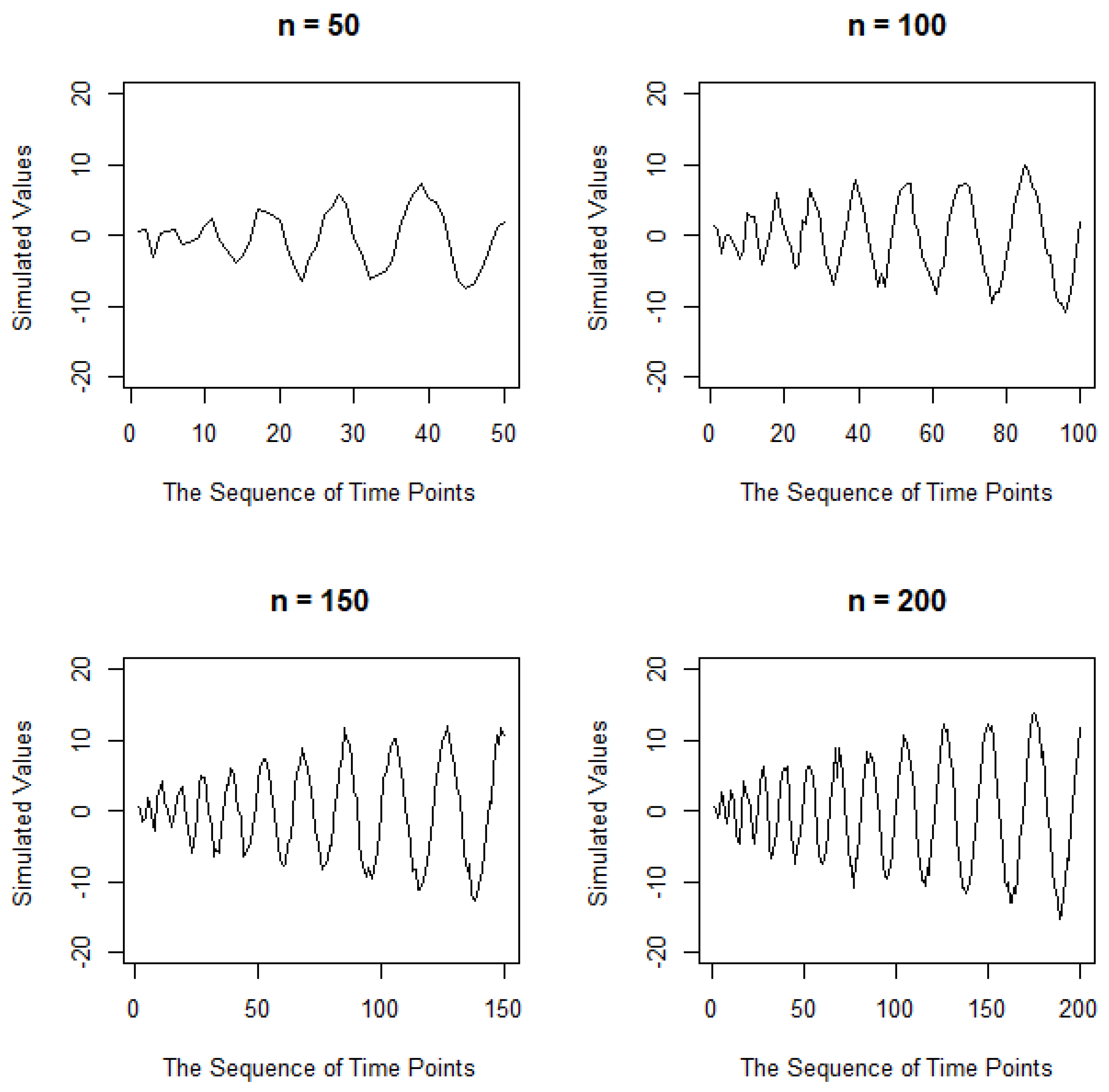
This function simulates the cyclic patterns in terms of time series data, as follows:

$$y_t=\hspace{0.17em}\hspace{0.17em}\hspace{0.17em}\sqrt{x_t}\hspace{0.17em}\hspace{0.17em}\sin \left(2\pi \left[1+\sqrt{x_t}\right]\right)+{\epsilon }_t\hspace{0.17em}\hspace{0.17em},\hspace{0.17em}\hspace{0.17em}t=1,2,\dots ,n,$$

where $\hspace{0.17em}{\epsilon }_t$ is an error term via the normal distribution with mean zero and standard deviations 1, 3, 5, and 7, as shown in Figure 1, Figure 2, Figure 3 and Figure 4.

Figure 1. The time series plot of cyclic patterns with a standard deviation of one for several sample sizes.

Figure 2. The time series plot of cyclic patterns with a standard deviation of three for several sample sizes.

Figure 3. The time series plot of cyclic patterns with a standard deviation of five for several sample sizes.

Figure 4. The time series plot of cyclic patterns with a standard deviation of seven for several sample sizes.

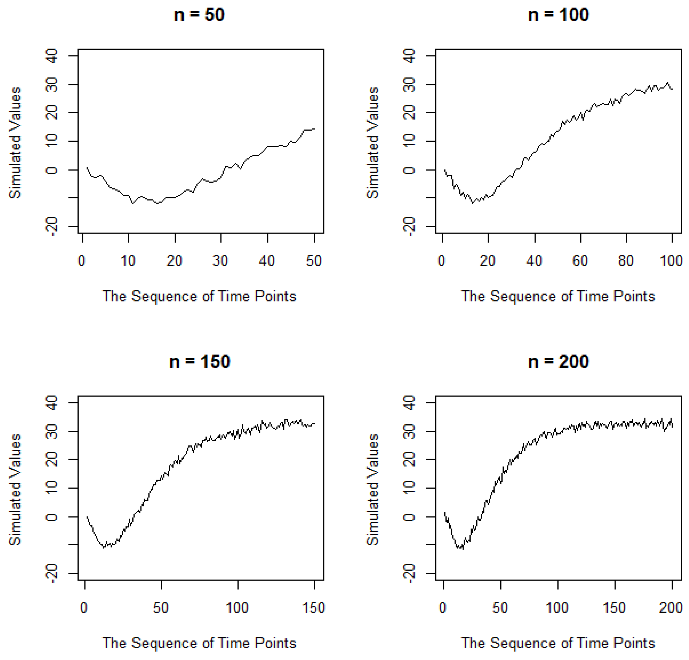
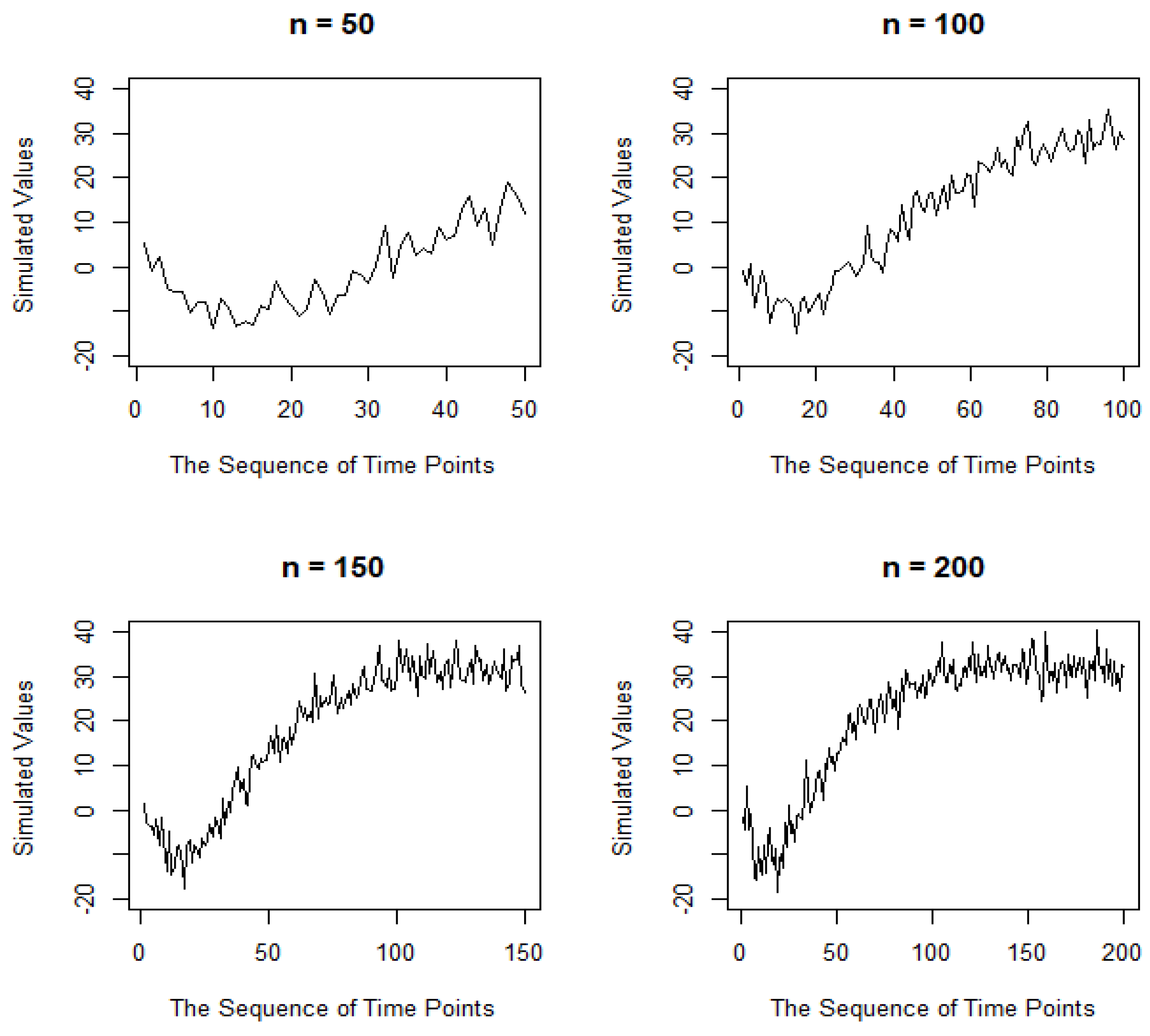
With the use of nonlinear forms, the dependent variables are simulated from the following function:

$$y_t=3\sqrt{x_t}\hspace{0.17em}\hspace{0.17em}\sin \left(2\pi \left[{\displaystyle \frac{1+30}{x_t+30}}\right]\right)+{\epsilon }_t\hspace{0.17em}\hspace{0.17em},\hspace{0.17em}\hspace{0.17em}t=1,2,\dots ,n,$$

where $\hspace{0.17em}{\epsilon }_t$ is an error term via the normal distribution with mean zero and standard deviations 1, 3, 5, and 7, as shown in Figure 5, Figure 6, Figure 7 and Figure 8.

Figure 5. The time series plot of nonlinear forms with a standard deviation of one for several sample sizes.

Figure 6. The time series plot of nonlinear forms with a standard deviation of three for several sample sizes.

Figure 7. The time series plot of nonlinear forms with a standard deviation of five for several sample sizes.

Figure 8. The time series plot of nonlinear forms with a standard deviation of seven for several sample sizes.

The performance of estimation is compared by average mean square error (AMSE) as follows:

$$AMSE=\hspace{0.17em}\hspace{0.17em}\hspace{0.17em}{\displaystyle \frac{1}{m}}{\displaystyle \sum _{h=1}^{m}MS{E}_h}\hspace{0.17em},\hspace{0.17em}\hspace{0.17em}h=1,2,\dots ,m,$$

where $m$ is the number of replications. The mean square error (MSE) is computed by

$$MSE={\displaystyle \frac{{\displaystyle \sum _{i=1}^n{(y_i-{\widehat{y}}_i)}^2}}{n}}$$

where $y_i$ is the dependent variable, and ${\widehat{y}}_i$ is the estimated dependent variable from nonparametric regression methods.

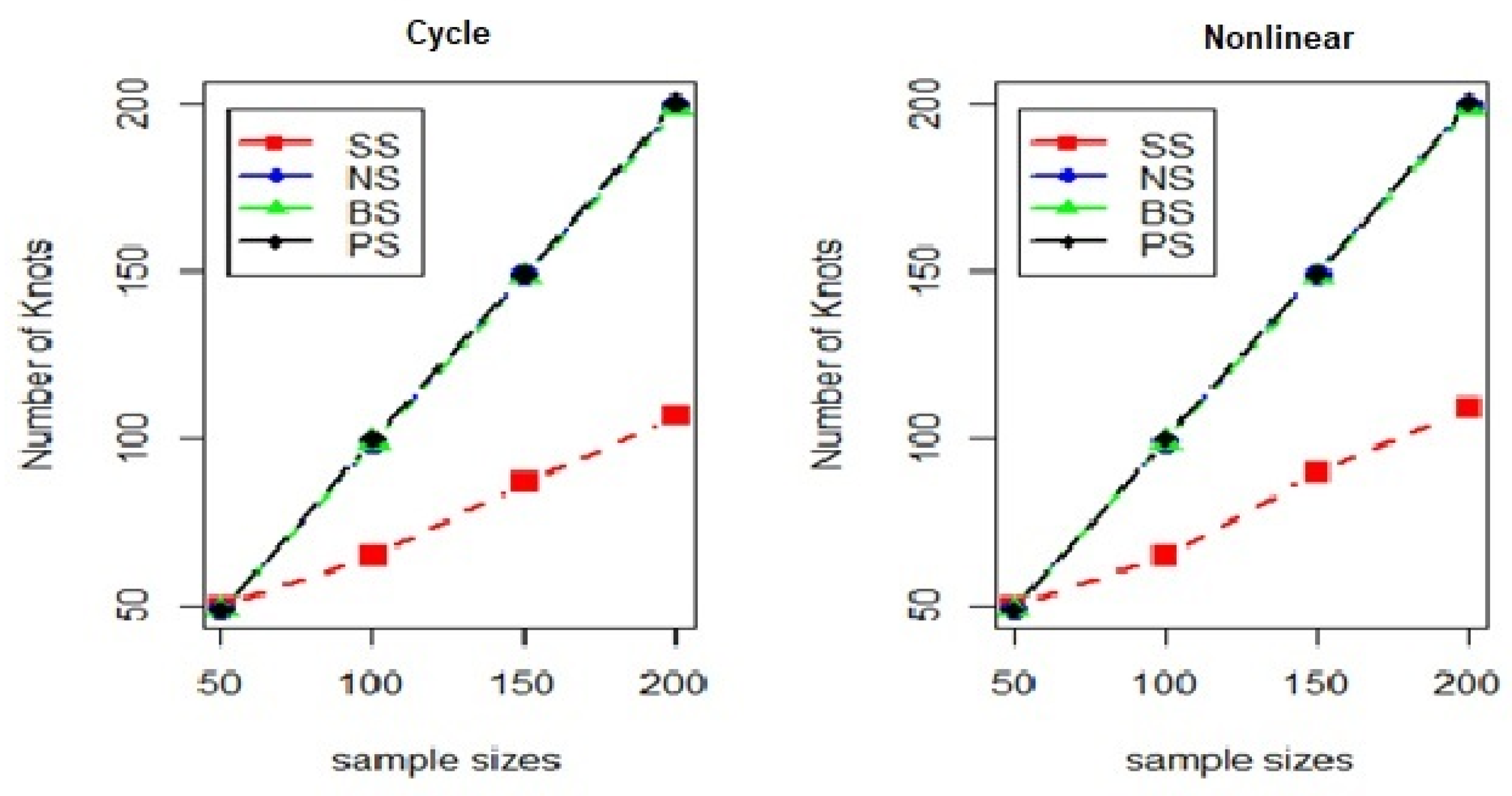
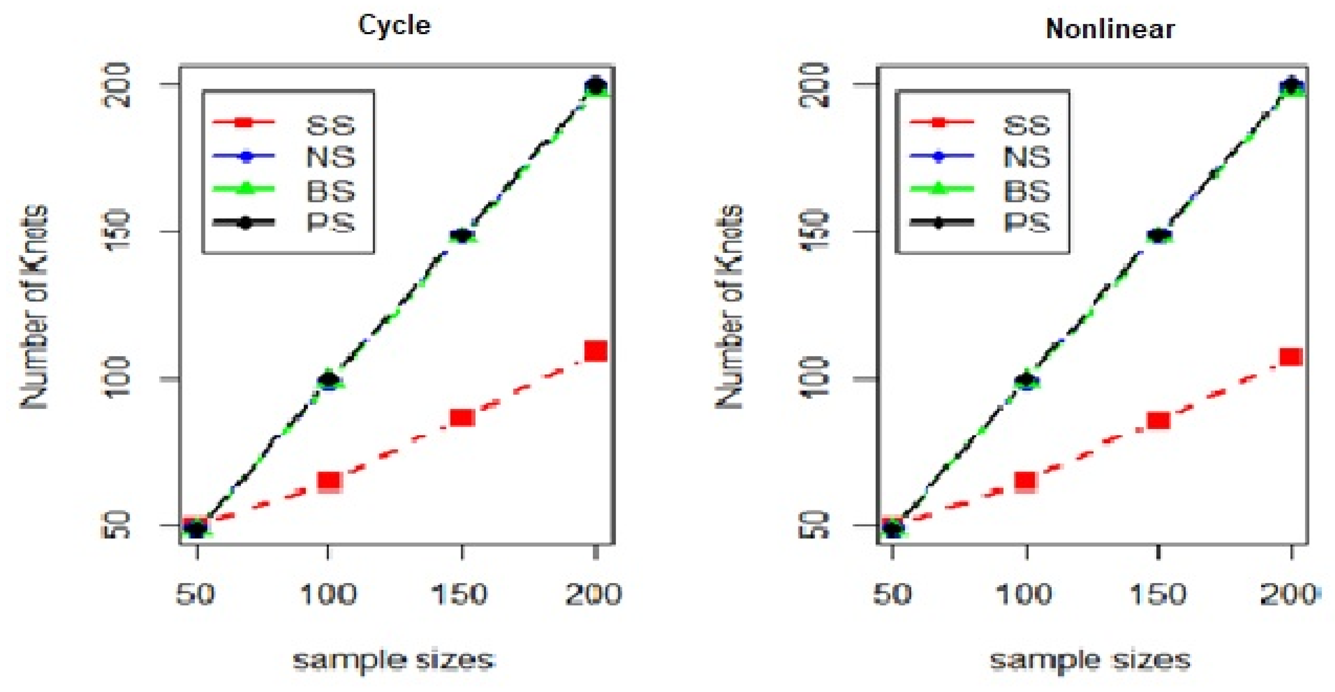
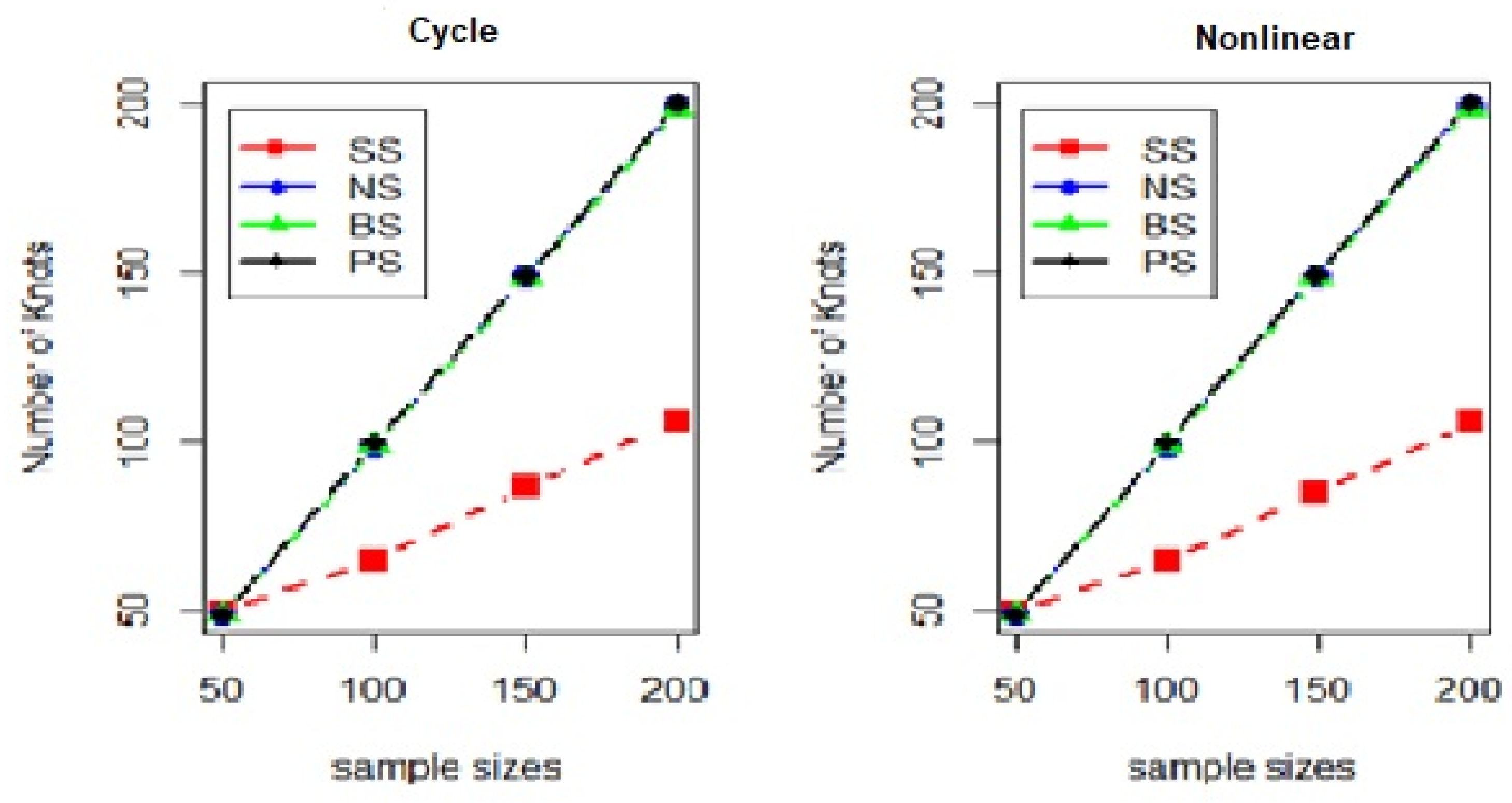
The simulation analysis comprises the average mean square error (AMSE) and the mean of the knot from smoothing spline (SS), natural cubic spline (NS), B-splines (BS), and penalized spline (PS) under standard deviation of error as 1, 3, 5, and 7, as presented in Table 1, Table 2, Table 3 and Table 4. To illustrate, the number of knots can be plotted using several methods and sample sizes, as shown in Figure 9, Figure 10, Figure 11 and Figure 12.

Table 1. The average mean square error (AMSE) and the mean of the knot (Knot) for the standard deviation of one.

n	Method	Cycle		Nonlinear
		MSE	Knot	MSE	Knot
50	SS	8.73 × 10−21	50	3.26 × 10−20	50
	NS	1.05 × 10−28	49	2.52 × 10−28	49
	BS	2.56 × 10−25	49	9.00 × 10−25	49
	PS	1.26 × 10−3	49	4.69 × 10−3	49
100	SS	0.11	65	0.36	65
	NS	5.07 × 10−28	99	2.35 × 10−27	99
	BS	5.23 × 10−18	99	2.15 × 10−17	99
	PS	1.12 × 10−11	100	3.74 × 10−11	100
150	SS	0.15	87	0.46	90
	NS	6.93 × 10−27	149	3.54 × 10−26	149
	BS	4.71 × 10−4	148	1.84 × 10−3	148
	PS	4.21 × 10−4	149	1.46 × 10−3	149
200	SS	0.16	107	0.49	109
	NS	1.09 × 10−26	199	7.37 × 10−26	199
	BS	6.13 × 10−4	198	2.31 × 10−3	198
	PS	6.52 × 10−11	200	2.07 × 10−10	200

Remark: Bold text meaning the lowest AMSE.

Table 2. The average mean square error (AMSE) and the mean of the knot (Knot) for the standard deviation of three.

n	Method	Cycle		Nonlinear
		MSE	Knot	MSE	Knot
50	SS	7.85 × 10−20	50	2.93 × 10−19	50
	NS	9.30 × 10−28	49	3.42 × 10−28	49
	BS	2.31 × 10−24	49	8.08 × 10−24	49
	PS	1.14 × 10−2	49	4.19 × 10−2	49
100	SS	0.95	65	3.26	65
	NS	4.51 ×10−27	99	2.74 × 10−27	99
	BS	4.70 × 10−17	99	1.93 × 10−16	99
	PS	1.01 × 10−10	100	3.35 × 10−10	100
150	SS	1.32	87	4.14	86
	NS	6.23 × 10−26	149	3.71 × 10−26	149
	BS	4.24 × 10−3	148	1.66 × 10−2	148
	PS	3.79 × 10−3	149	1.31 × 10−2	149
200	SS	1.45	109	4.43	107
	NS	9.69 × 10−26	199	7.50 × 10−26	199
	BS	5.52 × 10−3	198	2.08 × 10−2	198
	PS	5.87 × 10−10	200	1.86 × 10−9	200

Remark: Bold text meaning the lowest AMSE.

Table 3. The average mean square error (AMSE) and the mean of the knot (Knot) for the standard deviation of five.

n	Method	Cycle		Nonlinear
		MSE	Knot	MSE	Knot
50	SS	2.18 × 10−19	50	8.14 × 10−19	50
	NS	2.59 × 10−27	49	5.19 × 10−28	49
	BS	6.40 × 10−24	49	2.25 × 10−23	49
	PS	3.16 × 10−2	49	0.12	49
100	SS	2.62	65	9.05	65
	NS	1.26 × 10−26	99	3.55 × 10−27	99
	BS	1.31 × 10−16	99	5.36 × 10−16	99
	PS	2.81 × 10−10	100	9.29 × 10−10	100
150	SS	3.66	87	11.5	85
	NS	1.73 × 10−25	149	4.07 × 10−26	149
	BS	1.18 × 10−2	148	4.06 × 10−2	148
	PS	1.05 × 10−2	149	3.64 × 10−2	149
200	SS	4.05	106	12.3	106
	NS	2.69 × 10−25	199	7.85 × 10−26	199
	BS	1.53 × 10−2	198	5.78 × 10−2	198
	PS	1.63 × 10−9	200	5.17 × 10−9	200

Remark: Bold text meaning the lowest AMSE.

Table 4. The average mean square error (AMSE) and the mean of the knot (Knot) for the standard deviation of seven.

n	Method	Cycle		Nonlinear
		MSE	Knot	MSE	Knot
50	SS	1.60 × 10−18	50	4.28 × 10−19	50
	NS	7.82 × 10−28	49	5.24 × 10−27	49
	BS	4.42 × 10−23	49	1.26 × 10−23	49
	PS	0.23	49	6.20 × 10−2	49
100	SS	17.7	64	5.20	65
	NS	4.77 × 10−27	99	2.47 × 10−26	99
	BS	1.05 × 10−15	99	2.56 × 10−16	99
	PS	1.82 × 10−9	100	5.50 × 10−10	100
150	SS	22.5	84	7.17	88
	NS	4.61 × 10−26	149	3.39 × 10−25	149
	BS	9.03 × 10−2	148	2.31 × 10−2	148
	PS	7.14 × 10−2	149	2.06 × 10−2	149
200	SS	24.1	106	7.88	106
	NS	8.46 × 10−26	199	5.28 × 10−25	199
	BS	0.11	198	3.00 × 10−2	198
	PS	1.01 × 10−8	200	3.19 × 10−9	200

Remark: Bold text meaning the lowest AMSE.

Figure 9. The plots of a number of knots with cycle and nonlinear forms for the standard deviation of one.

Figure 10. The plots of a number of knots with cycle and nonlinear forms for the standard deviation of three.

Figure 11. The plots of a number of knots with cycle and nonlinear forms for the standard deviation of five.

Figure 12. The plots of a number of knots with cycle and nonlinear forms for the standard deviation of seven.

From Table 1, Table 2, Table 3 and Table 4, the average mean square error (MSE) for the cyclic data differs slightly from that for the nonlinear data, particularly for the natural cubic spline, B-splines, and penalized spline methods. However, the average MSE for the smoothing spline is higher than that for the other methods, and the number of knots used is lower, as shown in Figure 9, Figure 10, Figure 11 and Figure 12. The number of knots for the various methods tends to approach the sample sizes. The average MSE increases as the standard deviation rises, indicating the impact on the model’s fitting performance. Despite the increase in sample sizes, the parameter estimation remained unaffected. The results also show that the natural cubic spline consistently outperforms the other nonparametric regression models.

4. Application with Real Data

Coal imports have played a significant role in Thailand’s energy sector, contributing to energy security, baseload power generation, cost-effectiveness, industrial use, and overall economic development. In recent years, estimating and forecasting coal imports has gained renewed attention as Thailand reassesses its energy strategies in light of environmental considerations. This study examines a dataset of Thailand’s coal imports consisting of 336 monthly records (in 1000 tons) from January 1996 to December 2023, sourced from https://www.eppo.go.th/index.php/th/energy-information/static-energy/coal-lignite (accessed on 1 October 2024). The dataset exhibits cyclic patterns, with a seasonal component and nonlinear trends, as shown in Figure 13.

Figure 13. The time series plot of Thailand’s coal imports.

The empirical analysis applies four nonparametric regression methods to estimate the smoothing function for Thailand’s coal imports. The independent variable is represented by a sequence of 336 months, while the dependent variable is the monthly coal volume (per 1000 tons). Mean square error (MSE) measures the differences between actual and estimated values, while mean absolute percentage error (MAPE) assesses the prediction accuracy in percentage terms. The precision of both estimation and forecasting is evaluated using MSE and MAPE. The equations for calculating MSE and MAPE are as follows:

$$MSE=\hspace{0.17em}\hspace{0.17em}\hspace{0.17em}{\displaystyle \frac{1}{324}}{\displaystyle \sum _{t=1}^{324}{(y_t-{\widehat{y}}_t)}^2}\hspace{0.17em},\hspace{0.17em}\hspace{0.17em}\hspace{0.17em}t=1,2,\dots ,324$$

and

$$MAPE={\displaystyle \frac{1}{12}}{\displaystyle \sum _{t=325}^{336}\frac{\left|y_t-{\widehat{y}}_t\right|}{y_t}}\times 100,\hspace{0.17em}\hspace{0.17em}\hspace{0.17em}t=325,\dots ,336.$$

The mean square errors (MSEs) and knots are approximated from the smoothing spline, natural cubic spline, B-splines, and penalized spline methods displayed in Figure 14.

Figure 14. The fitted nonparametric regression model of Thailand’s coal imports.

Based on the above figure, all methods’ fitted nonparametric regression models make it difficult to indicate the best-performing method, especially the natural cubic spline, B-splines, and penalized spline. Then, the mean square errors (MSEs) are used to investigate the outperformed method, with the results presented in Table 5.

Table 5. The mean square errors (MSEs) and knots for estimating nonparametric regression methods.

Smoothing Spline		Natural Cubic Spline		B-Splines		Penalized Spline
Knots	MSE	Knots	MSE	Knots	MSE	Knots	MSE
270	45,655.86	323	1.59 × 10−22	319	407.154	324	2623.95

Remark: Bold text meaning the lowest MSE.

Table 5 presents the optimal knots and MSE values for the smoothing spline, natural cubic spline, B-spline, and penalized spline methods. The natural cubic spline yielded the lowest MSE, indicating it is this dataset’s most accurate estimation method.

Following the estimation, these nonparametric regression models are used to forecast future values for the next 12 months, with MAPE calculated to assess the accuracy over the given period. Table 6 displays the actual data, predicted values, and MAPE for all four methods.

Table 6. The volume of coal imports per month, forecasting values for 12 months, and MAPE.

Volume Import of Coal per Month	Smoothing Spline	Natural Cubic Spline	B-Splines	Penalized Spline
2113.43	1909.525	2072.425	2114.723	2142.787
1487.66	1876.894	1518.439	1487.375	1470.478
1910.45	1638.946	1889.213	1910.499	1919.366
1180.10	1399.448	1193.553	1180.093	1176.000
1492.87	1178.200	1485.054	1492.871	1494.834
1220.24	1285.590	1224.397	1220.240	1218.536
1001.75	1514.348	999.728	1001.750	1004.446
2018.69	1647.792	2019.586	2018.690	2012.885
1578.92	1541.290	1578.558	1578.920	1599.190
1429.56	1338.419	1429.691	1429.560	1344.191
1036.85	1254.809	1036.809	1036.850	1161.381
1586.06	1506.089	1586.067	1586.060	1530.713
MAPE	16.193	0.617	0.0027	2.245

Note: MAPE is expressed as a percentage (%).

Table 6 shows that the B-splines method yielded the lowest MAPE, at 0.0027. While the natural cubic spline proved to be the most suitable method for estimating real data, B-splines outperformed it in forecasting future values, as shown in Figure 15.

Figure 15. Plot of actual data (o) and forecasts for 12 future periods.

Figure 15 compares four nonparametric regression methods—smoothing spline, natural cubic spline, B-splines, and penalized spline—for modeling Thailand’s coal imports over 12 months. Both the B-splines and penalized spline methods provide the closest fit to the actual data points, while the natural cubic spline also performs well, though with a smoother curve. In contrast, the smoothing spline shows more significant variation and deviates from the other methods, particularly around months 7 and 9. Overall, the B-splines and penalized spline methods offer the best fit for accurately forecasting coal imports.

5. Discussion

The simulated results are listed in Table 1, Table 2, Table 3 and Table 4, which are applied or conducted using the nonparametric regression model. The natural cubic spline outperforms the other methods across all sample sizes and standard deviations. However, the nonlinear form shows more accurate estimations than the cyclic patterns based on the mean square errors. Increasing sample sizes and standard deviations did not affect the estimation process, as the nonparametric methods allow for flexible interpolation and extrapolation through knots, making them versatile for various applications. Nonparametric regression is instrumental when linearity is not a reasonable assumption in the data.

Regarding the impact of knots in real datasets, the four nonparametric regression methods show an increasing number of knots for forecasting future data, as seen in Table 7. However, increasing the number of knots does not necessarily guarantee the best method, and time spent finding optimal knots may not always be justified. This study suggests that B-splines are more effective for forecasting future values, while smoothing splines, natural cubic splines, and penalized splines rely on the same knot approach described in [44]. Knots are specific points in the independent variable space where the relationship between the independent and dependent variables may shift. They are commonly used in spline-based nonparametric regression methods, such as cubic splines or piecewise linear regression, and offer distinct advantages in improving model flexibility and accuracy.

Table 7. The number of knots, mean square errors (MSEs), and mean absolute percentage errors (MAPE) for Thailand’s coal imports.

Knots	Smoothing Spline		Natural Cubic Spline		B-Splines		Penalized Spline
	MSE	MAPE	MSE	MAPE	MSE	MAPE	MSE	MAPE
50	64,267.07	18.964	67,975.98	18.214	68,841.11	18.484	68,176.65	19.302
100	48,361.70	16.902	55,395.93	17.832	51,953.11	15.032	55,592.10	18.189
150	47,548.64	16.193	38,866.37	17.374	37,474.80	13.119	38,814.00	17.128
200	47,548.64	16.193	27,793.03	12.615	28,495.20	12.035	27,889.22	13.113
250	47,548.64	16.193	17,646.52	10.694	16,872.12	8.606	17,636.56	10.835
300	47,548.64	16.193	7847.429	5.026	12,617.89	0.244	47,548.64	16.193

Note: MAPE is expressed as a percentage (%)

6. Conclusions

The significance of this study lies in its comparison of popular nonparametric regression methods, including smoothing splines, natural cubic splines, B-splines, and penalized splines, applied to both simulated data and a real-world dataset. Cyclic patterns and nonlinear forms are simulated across standard deviations and sample sizes. The natural cubic spline consistently achieves the lowest MSE for parameter estimation, demonstrating its effectiveness when applied to time series data. Additionally, using a real dataset, such as Thailand’s coal imports, produced similar fitted model results to those obtained from the simulated data. However, as Mineo et al. [45] noted, B-splines are particularly suitable for forecasting future values. Despite these advantages, nonparametric regression presents challenges, including the risk of overfitting, the need for larger sample sizes, and increased computational complexity. Ultimately, the choice between parametric and nonparametric regression methods depends on the characteristics of the data and the goals of the analysis.

Future research could focus on increasing the number of knots to improve model accuracy and exploring other nonparametric regression techniques, such as kernel smoothing or local polynomial regression. These methods could be tested on datasets with varying complexities. It will also be essential to consider computational efficiency for larger datasets and develop a broader range of error metrics, such as RMSE or MAE, to evaluate forecasting accuracy comprehensively.