Abstract
Time series forecasting plays a critical role in business planning by offering insights for a competitive advantage. This study compared three forecasting methods: the Holt–Winters, Bagging Holt–Winters, and Box–Jenkins methods. Ten datasets exhibiting linear and non-linear trends and clear and ambiguous seasonal patterns were selected for analysis. The Holt–Winters method was tested using seven initial configurations, while the Bagging Holt–Winters and Box–Jenkins methods were also evaluated. The model performance was assessed using the Root-Mean-Square Error (RMSE) to identify the most effective model, with the Mean Absolute Percentage Error (MAPE) used to gauge the accuracy. Findings indicate that the Bagging Holt–Winters method consistently outperformed the other methods across all the datasets. It effectively handles linear and non-linear trends and clear and ambiguous seasonal patterns. Moreover, the seventh initial configurationdelivered the most accurate forecasts for the Holt–Winters method and is recommended as the optimal starting point.
1. Introduction
Forecasting is critical in decision making across various sectors, from business and finance to government and education. It involves predicting future events, trends, and behaviors based on historical data, current conditions, and analytical models. Accurate forecasting enables organizations to plan more effectively, mitigate risks, and capitalize on opportunities. It is essential for optimizing business operations and significantly benefits public and private sector organizations.
Common forecasting techniques include the smoothing method and the Box–Jenkins method. The Holt–Winters method is known for its simplicity, ease of implementation, and strong performance in time series forecasting with linear trends and seasonality. Several studies have examined how different initial settings affect the method’s accuracy. Suppalakpanya et al. [1] compared four initial settings of the Holt–Winters and Extended Additive Holt–Winters (EAHW) methods to forecast Thailand’s crude palm oil prices and production. Their findings revealed significant differences in the MAPE values based on the starting settings of both methods.
Researchers have sought to identify the optimal initial settings for the Holt–Winters model to improve the prediction accuracy. Hansun [2] introduced new estimation rules for unknown parameters in the Holt–Winters multiplicative model, while Trull [3] proposed alternative initialization methods for forecasting models with multiple seasonal patterns. Wongoutong [4] compared new default settings with the original Holt–Winters and Hansun initial settings, finding that the new settings produced the best results across all ten datasets.
The Bagging Holt–Winters method is an advanced forecasting technique that integrates the strengths of the Holt–Winters method with bootstrap aggregation (bagging). This hybrid approach enhances the accuracy and robustness of forecasts, particularly in complex or noisy data environments. Bergmeir et al. [5] demonstrated significant improvements in forecasting monthly data using this technique. Dantas et al. [6] utilized the Bagging Holt–Winters method to forecast the air transportation demand, obtaining the best results in 13 out of 14 monthly time series.
The Box–Jenkins method is a foundational time series analysis technique, providing a theoretical and practical basis for advanced strategies such as the Seasonal ARIMA (SARIMA), Autoregressive Conditional Heteroskedasticity (ARCH)/Generalized Autoregressive Conditional Heteroskedasticity (GARCH), and state-space models. The method is particularly effective for short-term predictions. Tayib et al. [7] used the Box–Jenkins method to predict Malaysia’s crude palm oil production, finding reliable and accurate long-term forecasts. Alam [8] employed the Autoregressive Integrated Moving Average (ARIMA) and Artificial Neural Networks (ANNs) to forecast Saudi Arabia’s imports and exports, demonstrating the appropriateness of both methods for these tasks.
Therefore, this research employed the Holt–Winters exponential smoothing method with seven initiations, the Bagging Holt–Winters method, and the Box–Jenkins method to model ten monthly time series data with trends and seasonality. The criteria used to evaluate the models for the training data were the RMSE and MAPE, while only the MAPE was used for the testing data. The model with the lowest value was chosen.
2. Related Work
Numerous methodologies have been developed to improve the accuracy of time series forecasting. This section reviews the fundamental approaches used in this study: the Holt–Winters method, the Bagging Holt–Winters method, and the Box–Jenkins method.
The Holt–Winters exponential smoothing technique is widely applied for forecasting data with trend and seasonal components. It includes additive and multiplicative models. Previous research, such as that by Suppalakpanya et al. [1], has explored how different initial settings can enhance the forecasting accuracy of this method.
The Bagging Holt–Winters method combines bootstrap aggregation with the Holt–Winters model to improve the forecast stability and accuracy. This technique is handy for datasets with non-linear trends or ambiguous seasonality. Dantas et al. [6] demonstrated this method’s effectiveness in various forecasting scenarios.
The Box–Jenkins methodology, commonly called ARIMA modeling, is another cornerstone in time series forecasting that is particularly effective for short-term predictions. This method focuses on fitting an ARIMA model to stationary data by identifying patterns in the autocorrelation and partial autocorrelation functions. Studies such as those by Tayib et al. [7] and Alam [8] have highlighted the robustness of the Box–Jenkins method in various forecasting applications, including crude palm oil production and trade volumes. Lee et al. [9] employed the Box–Jenkins method to predict crude oil purchases in the U.S.A. and Europe and found that the results were incredibly accurate.
Forecasting air transportation demand has become increasingly important due to the global rise in air traffic [10]. Himakireeti and Vishnu [11] provided a detailed process for predicting airline seat occupancy using the ARIMA model. Al-Sultan et al. [12] used the ARIMA and other methods to forecast passenger volumes at Kuwait International Airport. Similarly, Hopfe et al. [13] used neural network models to forecast short-term passenger flows at U.S. airports during the COVID-19 pandemic.
Thailand’s export sector in international trade, especially in agriculture and electronics, is vital to its economic growth. The accurate forecasting of export values is essential for financial planning and policy making. Studies such as those by Ghauri et al. [14] and Kamoljitprapa et al. [15] have applied the ARIMA and Holt–Winters models to predict import and export volumes, using error metrics such as the RMSE and MAE (Mean Absolute Error) for evaluation.
This study aims to assess the impact of varying initial settings within the Holt–Winters method on the forecasting accuracy across different datasets with trends and seasonality. It also investigates whether the Bagging Holt–Winters method significantly improves the forecast accuracy compared to the traditional Holt–Winters and Box–Jenkins methods. Additionally, it seeks to identify the characteristics of time series where the Holt–Winters method, Box–Jenkins method, and Bagging Holt–Winters method each outperform the others regarding the forecasting accuracy.
3. Data Collection and Methodology
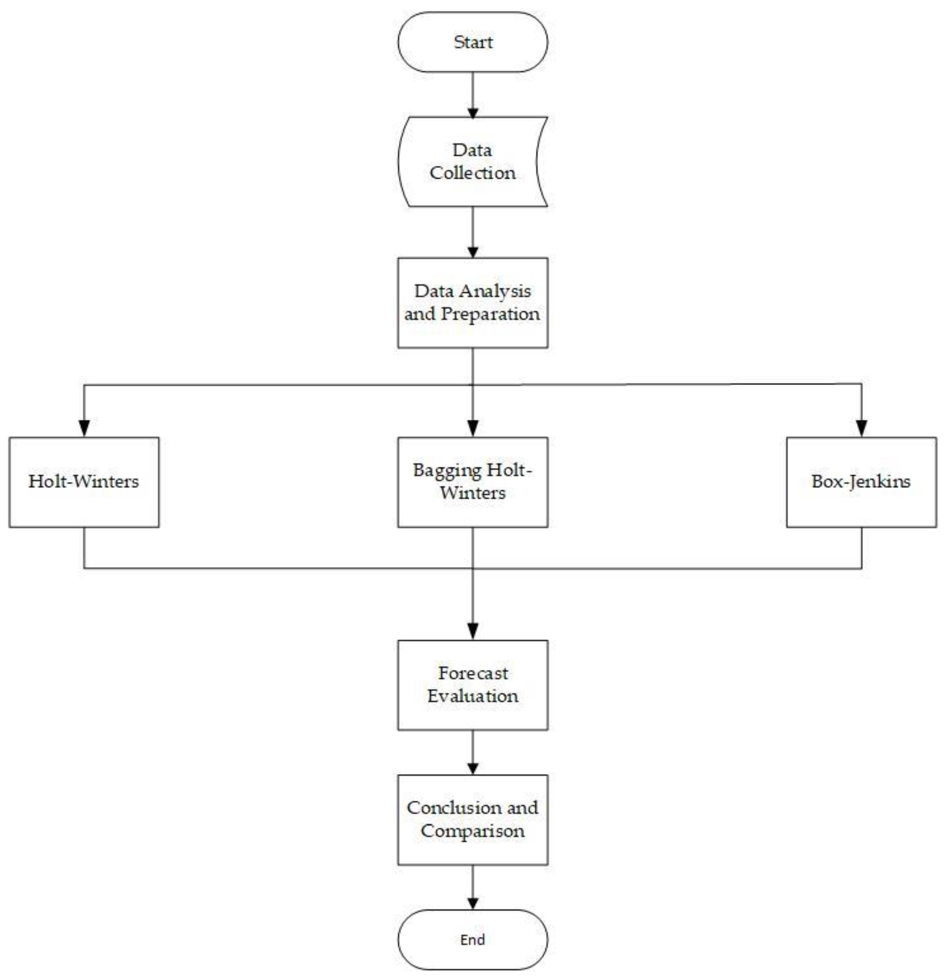
The methodological framework of this study consisted of five key steps, as illustrated in Figure 1.
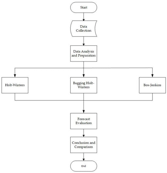
Figure 1.
Methodological framework for this study.
- Data Collection
Thailand’s exports contribute 75% to its Gross Domestic Product (GDP), while tourism revenue accounts for 17.7%. Data on exports and tourism were collected from various sources. This research selected 10 time series (TS) datasets with different trends and seasonality. The details of the ten datasets are provided in Table 1. The data sources were as follows:

Table 1.
Descriptions of the datasets used in this study.
- -
- TS1–TS6: Airports of Thailand Public Company Limited
- -
- TS7: The Information and Communication Technology Center, Office of the Permanent Secretary of the Ministry of Commence, in cooperation with the Thai Customs Department
- -
- TS8: Customs Department, Ministry of Finance
- -
- TS9–TS10: Office of Agricultural Economics, Ministry of Agriculture
- 2.
- Data Analysis and Preparation
The collected data were cleaned and preprocessed, focusing on identifying trends and seasonal patterns to ensure their appropriateness for the forecasting models.
- 3.
- Forecasting Model Development
Several forecasting methods were employed to analyze the data, including the following:
- -
- The Holt–Winters exponential smoothing method, initialized with seven initializations for both additive and multiplicative models;
- -
- The Bagging Holt–Winters method, which utilized the original initializations along with moving block bootstrap techniques, varying the block size (p) between 2 and 12 for both the additive and multiplicative models;
- -
- The Box–Jenkins method, which is a model based on autoregressive and moving-average components.
- 4.
- Forecast Evaluation
The accuracy of each forecasting model was assessed using the RMSE and MAPE. These metrics allowed for a clear comparison of the model performance:
- 5.
- Conclusion and Comparison
The study compared the models to determine which provided the most accurate forecasts for each dataset. Additionally, it examined the conditions under which specific models performed better, offering insights into their relative effectiveness.
3.1. The Holt–Winters Method
The Holt–Winters exponential smoothing method is suitable for linear trends and seasonality, with two variations: additive and multiplicative models. The choice between these models depends on whether the seasonal fluctuations are constant (additive) or proportional to the time series level (multiplicative) [16]. The forecasting and smoothing equations are presented in Table 2.

Table 2.
Forecasting and smoothing equations for the level, growth rate, and seasonality.
is the forecast value at period t, while represents the estimated level for the same period. indicates the growth rate at period t. and represent the estimated seasonality at periods t and t − L, respectively. L refers to the number of seasons per year. The term refers to the error in the time series at period t. Finally, and are smoothing constants, ranging between 0 and 1.
The Holt–Winters method requires initial values, which this research categorized into seven distinct patterns. Equation (1) defines the level component of patterns 1–5 for both additive and multiplicative models:
Equation (2) defines the level component for patterns 6 and 7:
Table 3 defines the growth rate of patterns 1 through 7. Equations (3) and (4) explain the seasonal factors for the additive and multiplicative models of patterns 1–6, respectively:

Table 3.
The growth rates for the seven patterns.
Seasonal factor pattern 7 is calculated using the ratio-to-moving-average method, which breaks the time series into three components: level, growth rate, and seasonality. However, only the seasonality component is used in this context [4].
Hansun [2] and Wongoutong [4] applied their method to the multiplicative Holt–Winters model. In contrast, this study applied their techniques to the additive and multiplicative Holt–Winters models. The smoothing parameters were estimated, and the RMSE was minimized using the Solver tool in Microsoft Excel version 365.
3.2. The Bagging Holt–Winters (BHW) Method
The Bagging Holt–Winters method is a four-step process:
Step 1: Decomposition. This step decomposes the time series into trend and seasonal components and residuals using the ratio-to-moving-average method. The remainder is expressed mathematically as shown in Equation (5):
where is the observed value and is the forecast value. The additive and multiplicative models for the forecast values are defined by Equations (6) and (7):
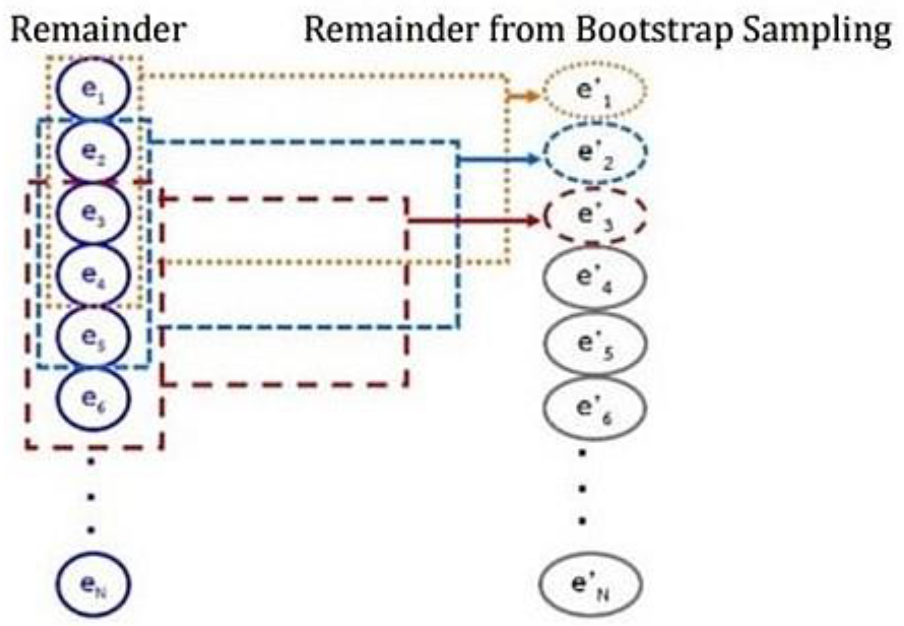
Step 2: Simulation. In this step, multiple new time series are generated using the moving block bootstrap method by resampling the random remainder with a block size (p) ranging from 2 to 12 periods, since the datasets consist of monthly data. For each random sampling block size (p), the remainder is randomized from period . The randomized remainder is combined with the estimated trend and the seasonal factor from Step 1 to create a new time series. This process is repeated 100 times.
Figure 2 illustrates an example of sampling the residual data using the moving block bootstrap method, with a block size set to p = 4.
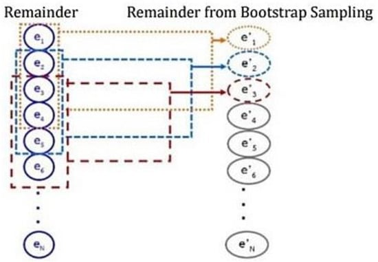
Figure 2.
Moving block bootstrap with random block size (p = 4).
Step 3: Forecasting
This step uses the new 100-time series constructed in Step 2 to model and forecast the time series using the Holt–Winters method. This method sets the level, growth rate, and seasonal factor according to pattern 1 (the original settings);
Step 4: Aggregation. This step uses the median to find the final forecast from 100 new time series forecast values for each random block size (p), since the median is good even though the data have outliers.
This research employed Visual Basic for Applications to model the Bagging Holt–Winters method.
3.3. The Box–Jenkins Method
The Box–Jenkins method is well known and widely used in modeling and forecasting. It employs the Autocorrelation Function (ACF) and Partial Autocorrelation Function (PACF) of stationary time series to identify the model. The method has a four-step process [21]:
Step 1: The ACF and PACF are employed to identify the tentative Box–Jenkins models;
Step 2: The parameters of the identified models are estimated from the historical data;
Step 3: The Box–Jenkins method uses various diagnostic methods to check the adequacy of the identified models. Sometimes, newly identified models are suggested and returned to Step 2;
Step 4: The final model predicts future time series values. Multiple models may be appropriate, and the optimal one is typically chosen based on the Akaike Information Criterion (AIC) and the Bayesian Information Criterion (BIC) [22], which are defined as follows:
where and RSS is the sum of the square residuals, k is the number of estimated model parameters, and m is the number of time series residuals. The optimal model is the one with the lowest AIC and BIC values.
The Box–Jenkins model is defined as follows [23]:
where is the order p of the autoregressive model; is the order P of the seasonal autoregressive model; is the order q of the moving-average model; is the order Q of the seasonal moving-average model.
is the actual data at period t, B is the backward shift operator, and θ0 is a constant. d and D are the numbers of regular and seasonal differences. L denotes the number of seasons per year. The error at time (t) is statistically independent and has a normal distribution with a zero mean and constant variance.
This research employed Minitab 21.0 to analyze the Box–Jenkins model.
4. Result
4.1. Results from the Holt–Winters Method
The seven initial settings were applied to all ten datasets (TS1–TS10) for the additive and multiplicative Holt–Winters models. The results are presented in Table 4 and Table 5. According to Table 4, the original Holt–Winters settings (Pattern 1) produced mid-range results compared to the other patterns. Pattern 2 yielded the poorest results for the additive and multiplicative models across several datasets, including TS1–TS2, TS4, TS7, TS9–TS10, and the additive model for TS8.

Table 4.
The RMSEs of seven settings of the Holt–Winters method for TS1-TS10.

Table 5.
The RMSEs of the multiplicative Bagging Holt–Winters model for TS1–TS10.
When comparing the seven patterns of the multiplicative Holt–Winters model, pattern 7 achieved the lowest RMSE for all the datasets (TS1–TS10). Similarly, pattern 7 provided the minimum RMSE in eight out of ten datasets for the additive Holt–Winters model, with the exceptions being TS5 and TS6. For these two datasets, patterns 4 and 1 produced the lowest RMSEs for the additive Holt–Winters model, respectively. In the case of the multiplicative Holt–Winters model, pattern 7 yielded the lowest RMSE for datasets TS1–TS2, TS4–TS8, and TS10, while for the additive Holt–Winters model, pattern 7 gave the smallest RMSE for TS3 and TS9.
This study concluded that pattern 7 offers the most effective initial settings. Previous research by Hansun [2] and Wongoutong [4] focused only on initial settings for multiplicative models. However, researchers should explore both additive and multiplicative models, as the best results may be found in the additive model and not just in the multiplicative model.
4.2. Results from the Bagging Holt–Winters Method
The results of the multiplicative Bagging Holt–Winters models are presented in Table 5. The minimum Root-Mean-Square Error (RMSE) occurs at different block sizes (p) for each time series. Specifically, the lowest RMSE is found at p = 2 for TS5; p = 3 for TS8; p = 4 for TS1, TS3, and TS6; p = 5 for TS4; p = 6 for TS7; p = 11 for TS10; and p = 12 for TS2 and TS9. Table 6 outlines the results for the additive Bagging Holt–Winters models, where the minimum RMSE occurs at p = 2 for TS6 and TS7; p = 3 for TS1, TS2, TS3, TS5, and TS8; p = 4 for TS4; p = 11 for TS9; and p = 12 for TS10.

Table 6.
The RMSEs of the additive Bagging Holt–Winters model for TS1-TS10.
Table 5 and Table 6 demonstrate that for the additive Bagging Holt–Winters models, the minimum RMSE is consistently found at p = 2 for TS6, at p = 3 for TS1, TS2, TS3, TS5, and TS8, and at p = 4 for TS4. In contrast, the multiplicative Bagging Holt–Winters models yield the lowest RMSE at p = 6 for TS7, at p = 11 for TS10, and at p = 12 for TS9. These findings suggest that the optimal block size (p) typically falls between 2 and 6 for more extended time series data. In contrast, for medium-length time series data, the optimal p is often 11 or 12.
Table 7 provides the Mean Absolute Percentage Errors (MAPEs) for the additive and multiplicative Bagging Holt–Winters models. The results are consistent with those for the RMSE: for the multiplicative models, the minimum MAPE occurs at p = 2 for TS5; at p = 3 for TS8; at p = 4 for TS1, TS3, and TS6; at p = 5 for TS4; at p = 6 for TS7; at p = 11 for TS10; and at p = 12 for TS2 and TS9. For the additive models, the minimum MAPE occurs at p = 2 for TS6 and TS7; at p = 3 for TS1, TS2, TS3, TS5, and TS8; at p = 4 for TS4; at p = 11 for TS9; and at p = 12 for TS10.

Table 7.
The MAPEs of the multiplicative and additive Bagging Holt–Winters model for TS1–TS10.
In summary, Table 7 confirms that the additive Bagging Holt–Winters models achieved the lowest MAPE at p = 2 for TS6, at p = 3 for TS1, TS2, TS3, TS5, and TS8, and at p = 4 for TS4, while the multiplicative models achieved the lowest MAPE at p = 6 for TS7, at p = 11 for TS9, and at p = 12 for TS10. These results further reinforce the observation that the optimal block size for long-term time series data ranges between 2 and 6. In contrast, it is typically 11 or 12 for medium-length time series data.
Moreover, this study found that the Bagging Holt–Winters models employing circular block bootstrapping produced identical results for both the RMSE and MAPE. Thus, researchers may use either the RMSE or MAPE for model evaluation, as the results are equivalent.
4.3. Results from the Box–Jenkins Method
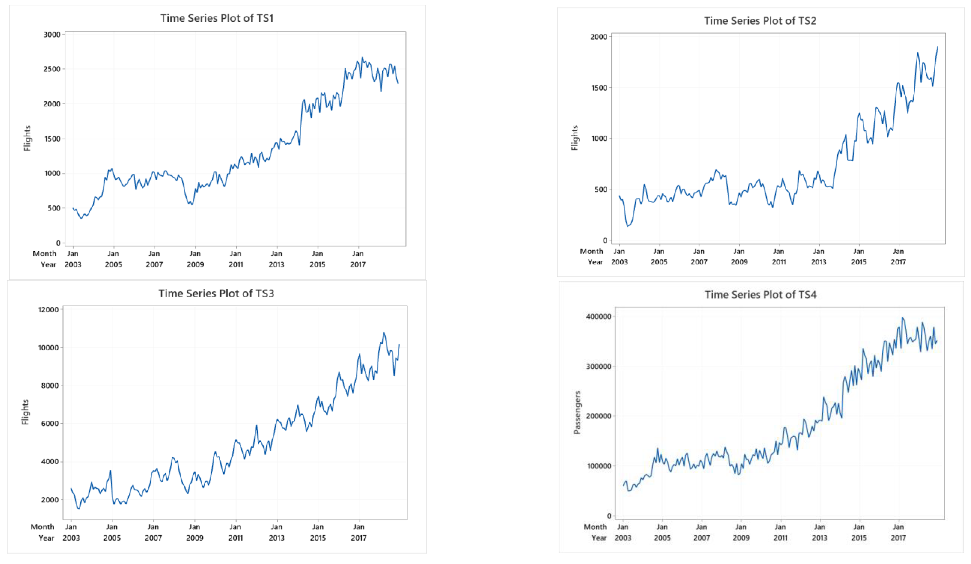
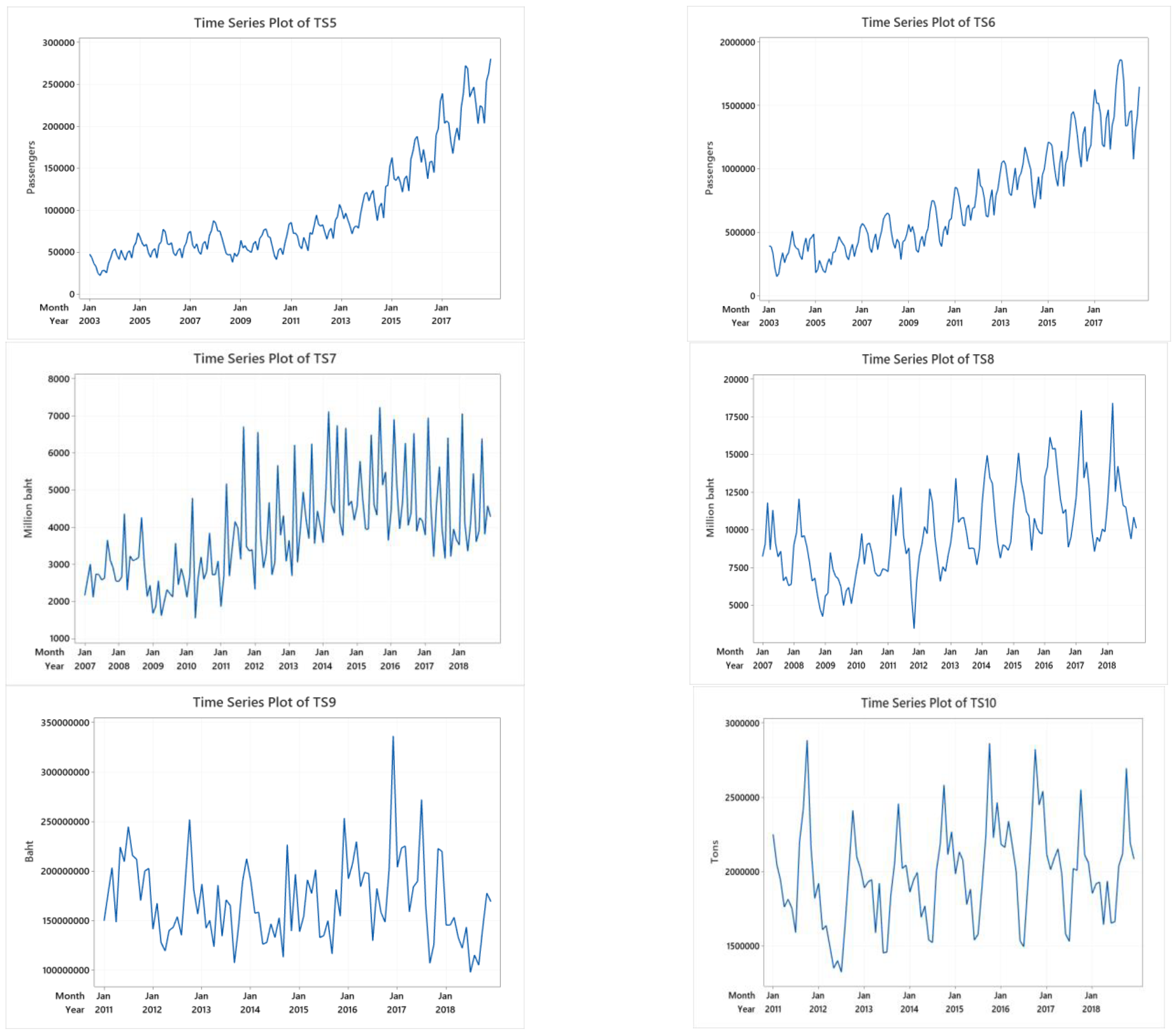
TS1–TS10 have both trend and seasonal variation, as shown in Figure 3. TS3, TS6, TS8, and TS10 show linear trends, and the rest show non-linear trends. TS3, TS5, TS6, TS8, TS9, and TS10 show clear seasonal patterns.
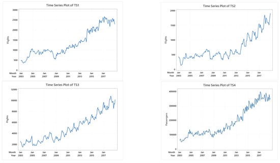
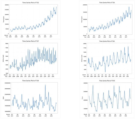
Figure 3.
The time series plots of TS1-TS10.
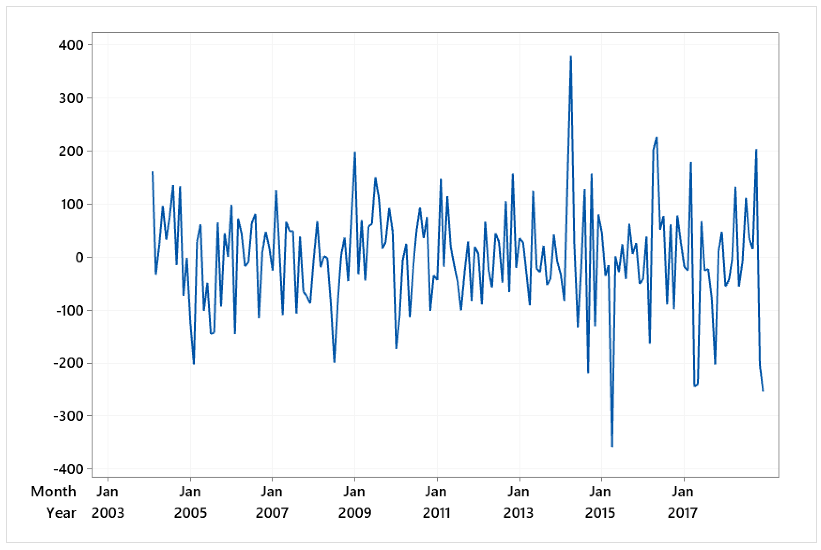
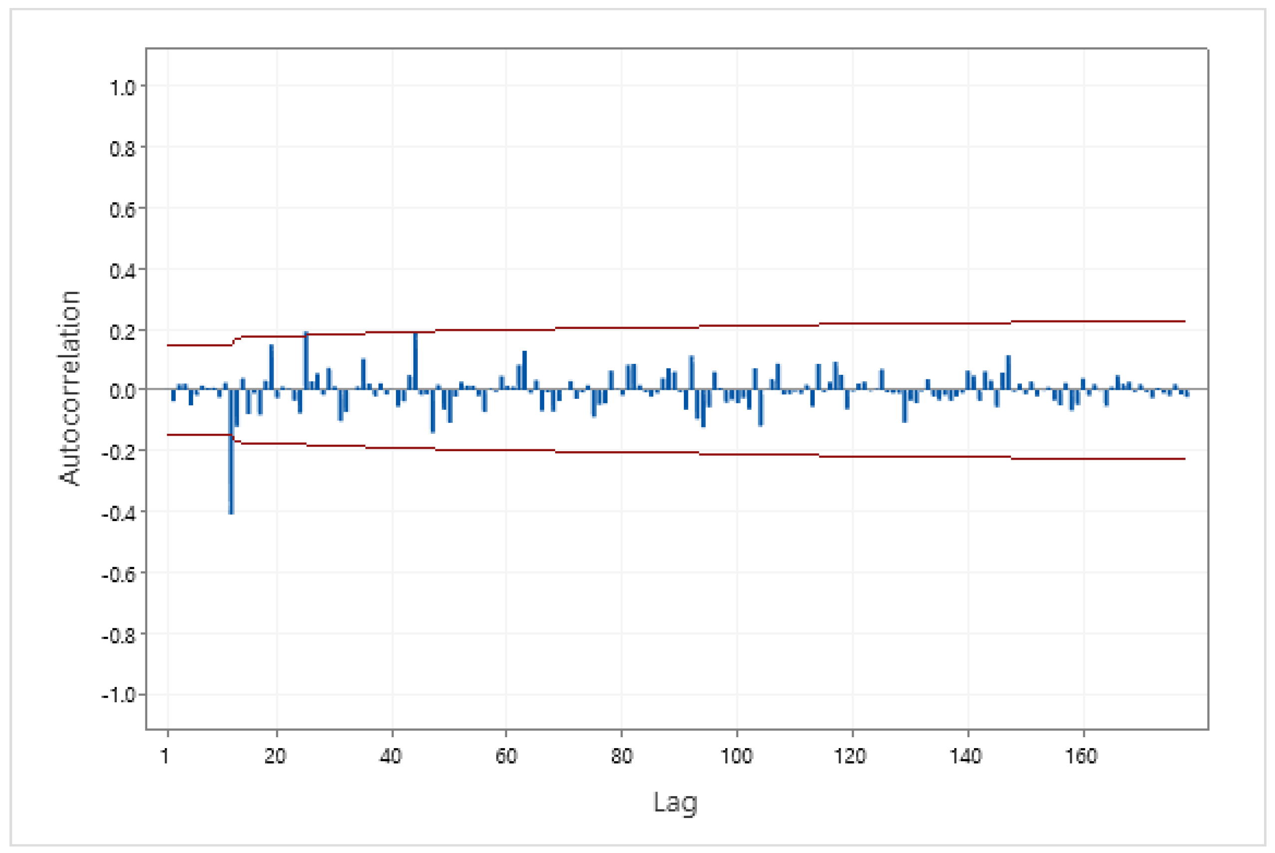
The Box–Jenkins stationary time series model can be determined from the ACF and PACF. To find the model for TS1, first, the time series was made stationary. This took one regular and one seasonal difference because TS1 shows trend and seasonality components. The plot of TS1 after one regular and one seasonal difference is shown in Figure 4. The time series plot of Figure 4 has a constant mean and variance, which implies that it is stationary. Second, the ACF and PACF of the stationary time series were plotted to identify the model. The ACF and PACF of the stationary time series are presented in Figure 5 and Figure 6. From Figure 5 and Figure 6, at lag 1–11, the ACF and PACF are equal to zero, which suggests a non-seasonal part . In the seasonal part, the ACF significantly differs from zero at lag 12, and the PACF at lag 12, 24, … is decreasing rapidly. This suggests seasonal model . The model for TS1 is .

Figure 4.
Time series plot of TS1 after one regular and one seasonal difference.
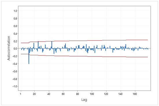
Figure 5.
The ACF of TS1 following one regular and one seasonal difference.
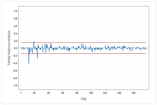
Figure 6.
The PACF of TS1 following one regular and one seasonal difference.
At the significance level of 0.05 by t-test, the parameter is statistically different from zero (p-value equals 0.00, smaller than 0.05), as shown in Table 8. The Box–Ljungtest shows that the model’s residuals are statistically independent, as the p-values for lags 12, 24, 36, and 48 are 0.949, 0.728, 0.902, and 0.864, which are all greater than 0.05.

Table 8.
Box–Jenkins model of TS1.
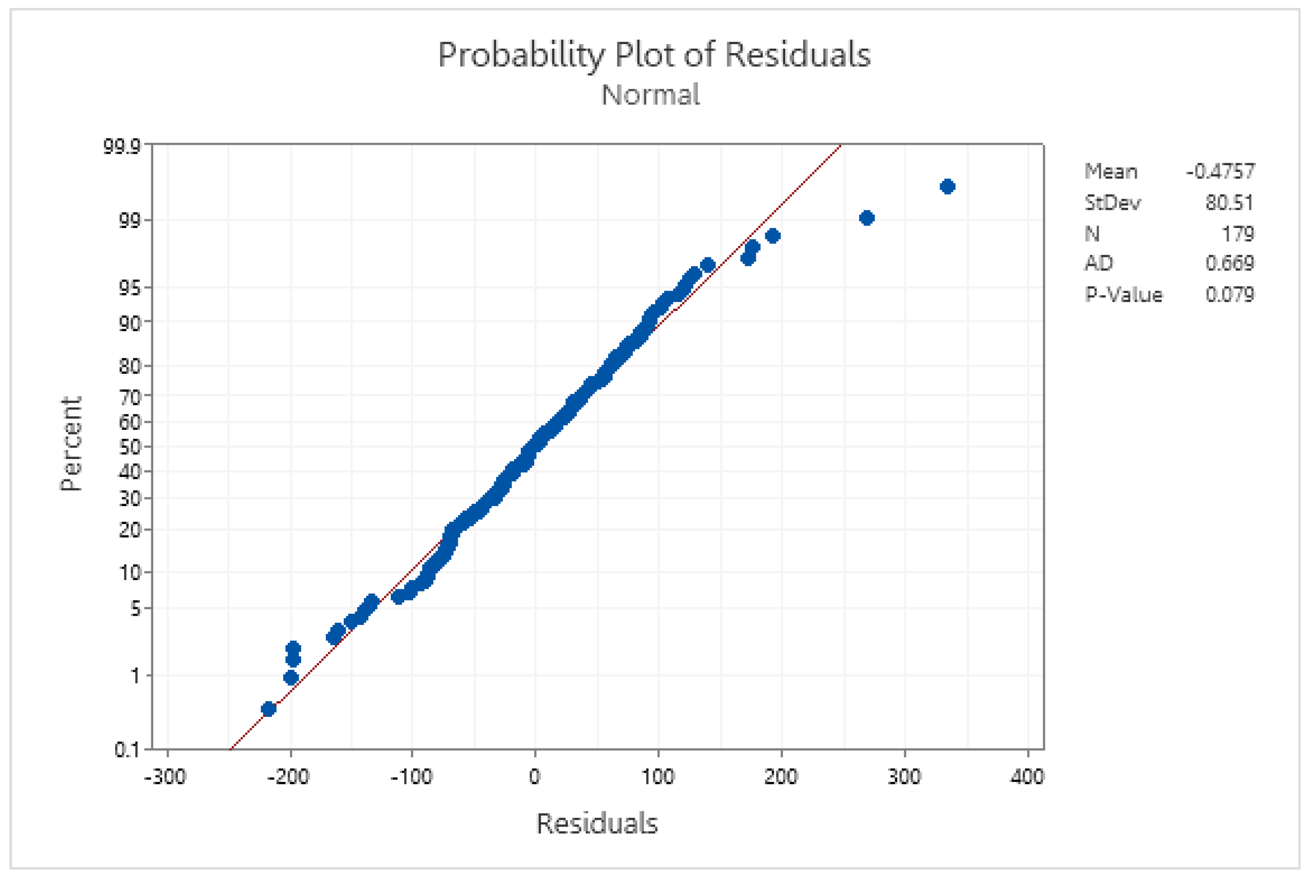
The model suits TS1. The Anderson–Darling normality test in Figure 7 shows that the model’s residuals follow a normal distribution because the p-value is greater than 0.05. In addition, also fits with TS1.

Figure 7.
The normality test for TS1 residuals.
All Box–Jenkins models that passed the diagnostic check, RMSE, AIC, and BIC for all datasets are shown in Table 9. The optimal model based on the minimum AIC and BIC for TS1, TS2, TS7, and TS8 is , and for TS3, it is . The best model for TS4, TS9, and TS10 is . The optimal models for TS5 and TS6 are and , respectively.

Table 9.
RMSE, AIC, and BIC of Box–Jenkins models for TS1-TS10.
The optimal forecasting models from three forecasting methods with the RMSE and MAPE of the training set can be seen in Table 10. The Bagging Holt–Winters method provided the optimal results for all the datasets. The multiplicative Bagging Holt–Winters method gave the optimal results for TS7, TS9, and TS10. The additive Bagging Holt–Winters method gave the optimal results for TS1–TS6 and TS8. The Box–Jenkins method performed better than the Holt–Winters pattern 7 for TS3, TS7, and TS8. The Holt–Winters pattern 7 gives better results for the remaining datasets than the Box–Jenkins method. Initializing with pattern 7 can increase the efficiency of the Holt–Winter method and potentially produce better results than the Box–Jenkins method.

Table 10.
RMSEs and MAPEs from three forecasting methods for the training set.
The best results of the Holt–Winters method occurred in the additive model, as shown in Table 10. However, the optimal results of the Bagging Holt–Winter method occurred in the multiplication model. In contrast, the optimal results of the Holt–Winter method appeared in the multiplicative model. However, the best results of the Bagging Holt–Winter method happened in the additive model. Therefore, the researcher should analyze the multiplicative and additive models for the Holt–Winters and Bagging Holt–Winters methods.
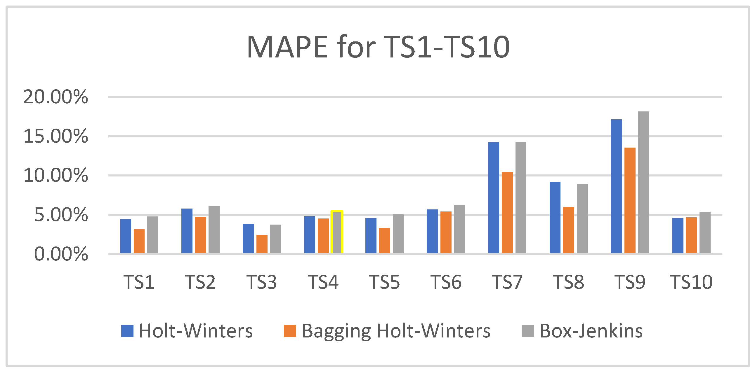
Bar charts of the MAPE values obtained from the three methods for each dataset can be seen in Figure 8. As shown, the MAPE values for TS6 and TS10 are nearly identical across all three methods. For TS1 to TS5, the MAPE values show slight differences, while for TS7 to TS9, the differences are more significant.
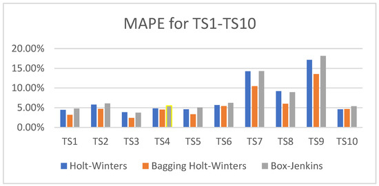
Figure 8.
The MAPE values from the three methods of 10 datasets.
The best prediction models and MAPEs for all the datasets are shown in Table 11. The additive Bagging Holt–Winters method with a random interval of p = 3 provided the best prediction model for TS1, TS2, TS3, TS5, and TS8, achieving MAPE values of 6.06%, 11.81%, 3.73%, 10.47%, and 7.70%, respectively. The additive Bagging Holt–Winters method with a random interval of p = 4 gave the best forecasting model for TS4 and obtained a MAPE of 11.66%. The additive Bagging Holt–Winters method with a random interval of p = 2 showed the best prediction model for TS6 and obtained a MAPE of 4.32%. The multiplicative Bagging Holt–Winters method with a random interval of p = 6 provided the best prediction model for TS7 and obtained a MAPE of 12.13%. The multiplicative Bagging Holt–Winters method with a random interval of p = 12 provided the best prediction model for TS9 and obtained a MAPE of 11.14%. The multiplicative Bagging Holt–Winters method with a random interval of p = 11 provided the best forecasting model for TS10 and obtained a MAPE of 5.78%. Table 10 shows that the Bagging Holt–Winters method gave good prediction values for all the datasets and gave MAPE values lower than 15%.

Table 11.
The optimal forecasting models and MAPE values for testing set of TS1-TS10.
5. Conclusions
This study compared three forecasting methods: the Holt–Winters method with different initial settings, the Bagging Holt–Winters method, and the Box–Jenkins method. Our findings demonstrate that the Bagging Holt–Winters method outperformed the others, providing more accurate results across all the datasets with linear and non-linear trends and clear and unclear seasonality patterns. The Bagging Holt–Winters approach offers improved efficiency through bootstrap aggregation, making it more robust for a wide range of data characteristics. Meanwhile, the Holt–Winters method with the pattern 7 initial settings gave the best result from all the datasets compared to the other patterns. It is the best choice for setting initial values for both the additive and multiplicative modeling of the Holt–Winters method.
The results of the Box–Jenkins method are better than those of the Holt–Winters method with the pattern 7 initial settings in some cases. The results from the three methods are nearly identical in the case of TS6 and TS10, which have linear trends and a clear patterns of seasonal factors. Therefore, the researcher can use one of these three methods if the time series has a linear trend and clear seasonality pattern.
Compared to the existing studies, our approach is more comprehensive in applying varied initial settings and includes bootstrap-based techniques. This allows for a better forecasting accuracy in scenarios with complex data patterns. However, this method requires more computational time and resources due to the multiple iterations involved in the bagging process. Additionally, while the Box–Jenkins method is still suitable for short-term predictions, it falls behind in accuracy compared to the Bagging Holt–Winters approach, especially for medium- to long-term forecasts.
The current study applied forecasting methods to datasets with trends and seasonality. Further research could use these methods in different domains, such as financial markets, climate modeling, or healthcare data, to evaluate their effectiveness across diverse fields. Furthermore, a simulation-based approach could provide a controlled environment to assess the forecasting performance under various conditions, including different data distributions and levels of noise. In addition, the General Forecast Error Second Moment (GFESM) [24] will be used as an additional evaluation metric alongside the RMSE and MAPE to provide a more comprehensive assessment of the forecast performance. This will enhance the robustness and reliability of the overall analysis.
Author Contributions
Conceptualization, S.B.; methodology, S.B.; software, S.B.; validation, S.B. and A.A.; formal analysis, S.B.; investigation, A.A.; resources, S.B.; data curation, S.B.; writing—original draft preparation, S.B. and A.A.; writing—review and editing, S.B. and A.A.; visualization, S.B.; supervision, S.B. and A.A. All authors have read and agreed to the published version of the manuscript.
Funding
This research was funded by King Mongkut’s Institute of Technology Ladkrabang Research Fund, School of Science, grant number 2565-02-05-009.
Data Availability Statement
Data are available at https://drive.google.com/drive/folders/1MEFKvO6kwr83YkyDNgUq1lBHfezSdsdH?usp=sharing (accessed on 20 September 2024).
Conflicts of Interest
The authors declare no conflicts of interest.
References
- Suppalakpanya, K.; Nikhom, R.; Booranawong, A.; Booranawong, T. An Evaluation of Holt-Winters Methods with Different Initial Trend Values for Forecasting Crude Palm Oil Production and Prices in Thailand. Suranaree J. Sci. Technol. 2019, 26, 13–22. [Google Scholar]
- Hansun, S. New estimation rules for unknown parameters on Holt-Winters multiplicative method. J. Math. Fundam. Sci. 2017, 49, 249–260. [Google Scholar] [CrossRef]
- Trull, O.; Garcia-Diaz, J.C.; Troncoso, A. Initialization Methods for Multiple Seasonal Holt-Winters Forecasting Models. Mathematics 2020, 8, 268. [Google Scholar] [CrossRef]
- Wongoutong, C. Improvement of the Holt-Winters Multiplicative Method with a New Initial Value Settings Method. Thail. Stat. 2021, 19, 280–293. [Google Scholar]
- Bergmeir, C.; Hyndman, R.J.; Benitez, J.M. Bagging Exponential Smoothing Methods using STL Decomposition and Box-Cox Transformation. Int. J. Forecast. 2016, 32, 303–312. [Google Scholar] [CrossRef]
- Dantas, T.M.; Oliveria, L.C.; Repolho, M.V. Air Transportation demand forecast through Bagging Holt-Winters methods. J. Air. Transp. Manag. 2017, 59, 116–123. [Google Scholar] [CrossRef]
- Tayib, S.A.M.; Nor, S.R.M.; Norrulashikin, S.M. Forecasting on the Crude Palm Oil Production in Malaysia using SARIMA Model. J. Phys. Conf. Ser. 2021, 1988, 012106. [Google Scholar] [CrossRef]
- Alam, T. Forecasting exports and imports through an artificial neural network and autoregressive integrated moving average. Decis. Sci. Lett. 2019, 8, 249–260. [Google Scholar] [CrossRef]
- Lee, J.Y.; Nguyen, T.-T.; Nguyen, H.-G.; Lee, J.Y. Towards Predictive Crude Oil Purchase: A Case Study in the USA and Europe. Energies 2022, 15, 4003. [Google Scholar] [CrossRef]
- Yang, C.H.; Lee, B.; Jou, P.H.; Lin, Y.D. Analysis and forecasting of international airport traffic volume. Mathematics 2023, 11, 1483. [Google Scholar] [CrossRef]
- Himakireet, K.; Vishnu, T. Air passengers occupancy prediction using the ARIMA Model. Int. J. Appl. Eng. Res. 2019, 14, 646–650. [Google Scholar]
- Al-Sultan, A.; Al-Rubkhi, A.; Alsaber, A.; Pan, J. Forecasting air passenger traffic volume: Evaluating time series models in long-term forecasting of Kuwait air passenger data. Adv. Appl. Stat. 2021, 70, 69–89. [Google Scholar] [CrossRef]
- Hopfe, D.H.; Lee, K.; Yu, C. Short-term forecasting airport passenger flow during periods of volatility: Comparative investigation of time series vs. neural network models. J. Air Transp. Manag. 2024, 115, 102525. [Google Scholar] [CrossRef]
- Ghauri, S.P.; Ahmed, R.R.; Streimikiene, D.; Streimikis, D. Forecasting exports and imports by using autoregressive (AR) with seasonal dummies and Box-Jenkins approaches: A case of Pakistan. Inz. Ekon.-Eng. Econ. 2020, 31, 291–301. [Google Scholar] [CrossRef]
- Kamoljitprapa, P.; Polsen, O.; Abdullahi, U.K. Forecasting of Thai international imports and exports using Holt-Winters and autoregressive integrated moving average models. J. Appl. Sci. Emerg. Technol. 2023, 22, 1–9. [Google Scholar] [CrossRef]
- Chatfield, C. The Analysis of Time Series, 5th ed.; Chapman & Hall: New York, NY, USA, 1996. [Google Scholar]
- Holt, C.C. Forecasting seasonals and trends by exponentially weighted moving averages. Int. J. Forecast. 2004, 20, 5–10. [Google Scholar] [CrossRef]
- Hyndman, R.J.; Athanasopoulos, G. Forecasting Principle and Practice, 2nd ed.; OTexts: Melbourne, Australia, 2018. [Google Scholar]
- Kalekar, P.S. Time Series Forecasting Using Holt-Winters Exponential Smoothing; Kanwal Rekhi School of Information Technology: Mumbai, India, 2004; pp. 1–13. [Google Scholar]
- Montgomery, D.C.; Jennings, C.L.; Kulahci, M. Introduction to Time Series Analysis and Forecasting, 2nd ed.; Wiley Series in Probability and Statistics; John Wiley &Sons: Hoboken, NJ, USA, 2008. [Google Scholar]
- Bowerman, B.L.; O’Connell, R.T.; Koehler, A.B. Forecasting, Time Series, and Regression: An Applied Approach, 4th ed.; Thomson Brooks/Cole: Pacific Grove, CA, USA, 2005. [Google Scholar]
- Koehler, A.B.; Murphree, E.S. A comparison of the Akaike and Schwarz Criteria for Selection Model Order. J. R. Stat. Soc. Ser. C. Appl. Stat. 1988, 37, 187–195. [Google Scholar]
- Box, G.E.P.; Jenkins, G.M.; Reinsel, G.C. Time Series Analysis Forecasting and Control; Prentice Hall: Hoboken, NJ, USA, 1994. [Google Scholar]
- Clements, M.P.; Hendry, D.F. On the Limitations of Comparing Mean Square Forecast Errors. J. Forecast. 1993, 12, 617–637. [Google Scholar] [CrossRef]
Disclaimer/Publisher’s Note: The statements, opinions and data contained in all publications are solely those of the individual author(s) and contributor(s) and not of MDPI and/or the editor(s). MDPI and/or the editor(s) disclaim responsibility for any injury to people or property resulting from any ideas, methods, instructions or products referred to in the content. |
© 2024 by the authors. Licensee MDPI, Basel, Switzerland. This article is an open access article distributed under the terms and conditions of the Creative Commons Attribution (CC BY) license (https://creativecommons.org/licenses/by/4.0/).

