Steady-State Harmonic Vibrations of Viscoelastic Timoshenko Beams with Fractional Derivative Damping Models

Abstract

Due to growing demands on newly developed products concerning their weight, sound emission, etc., advanced materials are introduced in the product designs. The modeling of these materials is an important task, and a very promising approach to capture the viscoelastic behavior of a broad class of materials are fractional time derivative operators, since only a small number of parameters is required to fit measurement data. The fractional differential operator in the constitutive equations introduces additional challenges in the solution process of structural models, e.g., beams or plates. Therefore, a highly efficient computational method called Numerical Assembly Technique is proposed in this paper to tackle general beam vibration problems governed by the Timoshenko beam theory and the fractional Zener material model. A general framework is presented, which allows for the modeling of multi-span beams with general linear supports, rigid attachments, and arbitrarily distributed force and moment loading. The efficiency and accuracy of the method is shown in comparison to the Finite Element Method. Additionally, a validation with experimental results for beam systems made of steel and polyvinyl chloride is presented, to illustrate the advantages of the proposed method and the material model.

1. Introduction

In the modeling process of real structures, many components are accurately described by simplified beam models, e.g., Euler-Bernoulli beam or Timoshenko beam theory, if two dimensions are significantly smaller than the third one. Therefore, a detailed analysis of this simplified structural elements is very important for practical applications; hence, a vast amount of literature on this topic is available, and many efforts have been devoted to understand the dynamics of beam models [1]. Due to advanced manufacturing processes, more complicated materials, especially viscoelastic materials [2], can be used in the product design to further improve dynamic characteristics, e.g., noise emission or vibration levels [3]. Therefore, it is necessary to also include such materials in the analysis of beam vibrations.

An accurate modeling of the behavior of such materials is required and various constitutive equations have been presented, e.g., the Kelvin–Voigt model [4], the Maxwell model [5], or the Zener model [6]. Increased possibilities in mechanical testing have shown that many materials with complex microstructure lead to a power-law signature in their creep and relaxation behaviors [7]. Even though recent studies, e.g., References [8,9], show that generalized versions of the classical models can lead to a good agreement with measured data for such materials, a large number of model parameters is required, which greatly hinders physical interpretation [7]. Therefore, so-called fractional time derivatives have been introduced in the constitutive equations, which are ideally suitable to model the viscoelastic behavior of materials [7,10] and allow for an accurate representation of the material behavior with a small number of parameters over a wide frequency range [11,12].

Several studies are reported in literature using fractional derivative damping models in the analysis of beam vibration problems. In Reference [13], a Timoshenko beam made of a viscoelastic material obeying a three-dimensional fractional derivative constitutive relation is analyzed. The Laplace transform is applied to compute the quasi-static response to a step loading, and the steady-state response to a periodic excitation of a simply-supported single-span beam is calculated by a modal approach. The Mellin transform is used by Pirrotta et al. [14] to compute the response of a viscoelastic Timoshenko beam under static loading conditions in the time domain. Additionally, an exact linking relationships between the response of a viscoelastic beam governed by the Euler–Bernoulli theory and the Timoshenko theory is established in Reference [2].

Usuki and Suzuki [15] derived the dispersion relations for Timoshenko beams made of different types of fractional viscoelastic materials and a beam made of polyvinyl chloride (PVC) foam is analyzed in detail. In Reference [12], the wave propagation method is applied to calculate the steady-state response of Euler-Bernoulli beams with a fractional Kelvin–Voigt material model. An analytical solution is obtained in the frequency domain and the effect of different fractional orders in the material damping model is analyzed. A comprehensive review on beam vibration problems with fractional viscoelastic material models can be found in Reference [16]. More recently, fractional damping models are also introduce in micro structures, e.g., micro beams [17] and nano beams [18], or anomalous materials [19].

Due to the fractional derivative material models, the solution of the resulting governing equations is more challenging compared to classical material models. Several computational techniques have been applied in literature to calculate natural frequencies, steady-state harmonic or transient responses of beam systems. Paunović et al. [20] presented a Galerkin approximation method combined with the Fourier integral transform method to calculate the vibrations of cantilever beams with several attached concentrated masses. In their work, the fractional order Kelvin–Voigt model is applied. In Reference [21], the Finite Element Method (FEM) is extended to analyze the vibrations of frames composed of Euler-Bernoulli beams with a fractional derivative damping model.

In this paper, the so-called Numerical Assembly Technique (NAT), which was proposed by Wu and Chou [22] in 1999 for the calculation of natural frequencies and mode shapes of beams with various attachments, is extended to general beam vibration problems governed by the Timoshenko beam theory with fractional viscoelastic material models. Since 1999, various modifications and extensions of NAT have been presented, e.g., free torsional vibrations of shafts [23], free vibrations of axially loaded beams [24], forced harmonic vibrations of beams with concentrated [25,26] and distributed loadings [27] or rotating beams [28,29,30].

Similar to the Transfer Matrix Method (TMM) [31] and the Dynamic Stiffness Method (DSM) [32], NAT uses (semi)-analytical solutions of the harmonic governing equations to fit the boundary conditions (and interface conditions if multi-span beams are investigated). An advantage of NAT compared to TMM and DSM is the simple introduction of specific particular solutions functions, which allows for the investigation of arbitrarily distributed loadings [27]. Since NAT is only applicable for free vibrations or harmonic excitations, the steady-state harmonic response of a general beam system is examined in this paper. However, using the Fourier transform technique, periodic or transient beam vibrations could also be investigated with NAT, e.g., Reference [20].

The outline of this paper reads as follows: First, a most general beam vibration problem is defined in Section 2, which includes a general linear model for the beam supports, rigid attachments, arbitrarily distributed loadings, and the introduction of the fractional Zener material model. In Section 3, the Numerical Assembly Technique is presented, and the analytical solutions of the Timoshenko beam theory with a fractional derivative damping model are derived. The exact solutions of the homogeneous governing equations and the particular solutions for point loadings are computed. For generally distributed loadings, an approximation by the Fourier extension method [33] is presented, and semi-analytical particular solutions are derived. A numerical validation of the proposed method is given in Section 4 using a numerical reference solution computed with the Finite Element Method. Additionally, a comparison with vibration measurements on two different beam structures made of steel and PVC is carried out. Finally, a conclusion is given in Section 5.

2. Problem Description

In this section, a general two-dimensional beam vibration problem is described, and different viscoelastic material models using fractional time derivatives are outlined. The Timoshenko beam theory is applied to model the beam segments including external viscous (air) damping.

2.1. General Viscoelastic Beam Vibration Problem

A general beam vibration problem is illustrated in Figure 1. It is assumed that the system is two-dimensional; therefore, no deformation occurs in the y-direction. Additionally, the system has no loading in the x-direction. The beam with total length L is split into M uniform and homogenous segments by $\left(N\right)$ stations. The first $\left(1\right)$ and last station $\left(N\right)$ represent the boundaries of the beam system. An additional station $\left(i\right)$ has to be introduced if a discontinuity in the system appears, either through a concentrated element, a change in the cross-section or the material parameters. The global coordinate of an intermediate station $\left(i\right)$ is given by $x=X_i$ and for each segment ℓ, a local coordinate system $(O_{\ell },x_{\ell },y_{\ell },z_{\ell })$ is defined. The origins of the local coordinate systems $O_{\ell }$ are coincident with the bending centers of each beam segment ℓ and are located at the associated left station $(x_{\ell }=(x-X_i)(i=\ell ))$.

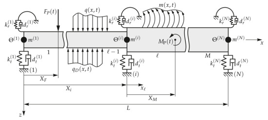
Figure 1. General two-dimensional beam vibration problem with distributed loading.

Each beam segment ℓ is straight and uniform with the length $L_{\ell }=(X_{i+1}-X_i)(i=\ell )$, complex Young’s modulus $E_{\ell }^{★}$, complex shear modulus $G_{\ell }^{★}$, density ${\rho }_{\ell }$, cross-section area $A_{\ell }$, and second moment of area about the y-axis $I_{\ell }$. It is assumed that the principal axes of all segments are aligned; therefore, the axial and bending deformations are decoupled [34].

The support at station $\left(i\right)$ of the beam is modeled by linear springs and dampers (translational springs $k_t^{\left(i\right)}$ or dampers $d_t^{\left(i\right)}$, rotational springs $k_r^{\left(i\right)}$ or dampers $d_r^{\left(i\right)}$) and rigid attachments by lumped masses $m^{\left(i\right)}$, and rotatory inertia ${\mathsf{\Theta }}^{\left(i\right)}$. The translational and rotational springs and dampers are linear, and, in the initial undeformed state, the springs are unstressed. All concentrated elements are connected to the beam at the bending center line. As illustrated in Figure 1, it is assumed that a general support, a rigid attachment, and a change in material and geometric properties appear simultaneously at each station. Every possible configuration at a station $\left(i\right)$ can be achieved by setting certain parameters of the supports or rigid attachments to zero or by keeping the material or geometric properties unchanged.

The external loading of the beam is modeled by point forces $F_P\left(t\right)$ at the local positions $X_F$, point moments $M_P\left(t\right)$ at the local positions $X_M$, distributed forces $q(x,t)$, and distributed moments $m(x,t)$. For steady-state harmonic vibrations at angular frequency $\omega$, the external loads can be defined by

$$q(x,t)=\tilde{q}\left(x\right){\mathrm{e}}^{\mathrm{j}\omega t},m(x,t)=\tilde{m}\left(x\right){\mathrm{e}}^{\mathrm{j}\omega t},F_P\left(t\right)={\tilde{F}}_P{\mathrm{e}}^{\mathrm{j}\omega t},M_P\left(t\right)={\tilde{M}}_P{\mathrm{e}}^{\mathrm{j}\omega t},$$

(1)

where t is the time, $\mathrm{j}=\sqrt{-1}$ the imaginary unit, and ${\tilde{F}}_P$, ${\tilde{M}}_P$, $\tilde{q}\left(x\right)$, and $\tilde{m}\left(x\right)$ are the complex amplitudes of the concentrated and distributed external loads. The external viscous (air) damping is denoted by $q_D(x,t)$.

2.2. Modeling of the Internal Material Damping

Although many solid materials are modeled as perfectly elastic, mainly by Hooke’s law, actual solids behave differently even for small stresses [35]. There is always at least a small dissipation of energy, even for metals [35].

In most beam theories, it is assumed that the transverse stress components ${\sigma }_{yy}$ and ${\sigma }_{zz}$ are very small compared to the axial stress component ${\sigma }_{xx}$ (${\sigma }_{xx}\gg {\sigma }_{yy}$, ${\sigma }_{xx}\gg {\sigma }_{zz}$). Consequently, it is assumed that the transverse stress components vanish (${\sigma }_{yy}\approx 0$, ${\sigma }_{zz}\approx 0$) [34]. Furthermore, only small deformations are considered; therefore, a linear material model can be applied. A perfectly elastic material is defined by Hooke’s law, which leads to the non-zero normal and shear stresses in a beam segment ℓ [34]:

$$\begin{array}{cc}\hfill {\sigma }_{xx}(x,z,t)& =E_{\ell }{\epsilon }_{xx}(x,z,t),\hfill \end{array}$$

(2)

$$\begin{array}{cc}\hfill {\sigma }_{xz}(x,t)& =G_{\ell }{\gamma }_{xz}(x,t),\hfill \end{array}$$

(3)

with $E_{\ell }$ the Young’s modulus, $G_{\ell }$ the shear modulus, ${\epsilon }_{xx}(x,z,t)$ the normal strain and ${\gamma }_{xz}(x,t)$ the shear strain. A transformation of Equations (2) and (3) into the frequency domain applying the Fourier transform results in

$$\begin{array}{cc}\hfill {\tilde{\sigma }}_{xx}(x,z,\omega )& =E_{\ell }{\tilde{\epsilon }}_{xx}(x,z,\omega ),\hfill \end{array}$$

(4)

$$\begin{array}{cc}\hfill {\tilde{\sigma }}_{xz}(x,\omega )& =G_{\ell }{\tilde{\gamma }}_{xz}(x,\omega ).\hfill \end{array}$$

(5)

A common approach to model the dissipative behavior of solid materials in the frequency domain is the constant hysteric damping model [36]. In this frequency independent model, the real-valued Young’s and shear modulus are simply replaced by complex moduli, which leads to

$$\begin{array}{cc}\hfill {\tilde{\sigma }}_{xx}(x,z,\omega )& =E_{\ell }^{★}{\tilde{\epsilon }}_{xx}(x,z,\omega ),\hfill \end{array}$$

(6)

$$\begin{array}{cc}\hfill {\tilde{\sigma }}_{xz}(x,\omega )& =G_{\ell }^{★}{\tilde{\gamma }}_{xz}(x,\omega ),\hfill \end{array}$$

(7)

with the complex Young’s modulus $E_{\ell }^{★}=E_{\ell }(1+\mathrm{j}{\eta }_{\ell }^E)$ and the complex shear modulus $G_{\ell }^{★}=G_{\ell }(1+\mathrm{j}{\eta }_{\ell }^G)$[36]. The loss factor ${\eta }_{\ell }^{•}$ defines the frequency-independent damping in this model. Although this simple model has certain advantages for numerical simulation, especially in finite element schemes, and approximates experimental results accurately in a limited frequency band, it leads to non-causal responses in the time-domain [36]. Therefore, more realistic damping models have been developed. Several of these models are based on so-called fractional time derivatives, which can be used in a wide frequency range and for a large class of materials, such as metals, glass, and especially polymers [11].

A very effective four-parameter model has been analyzed by Pritz [11], which is a generalized form of the so-called Zener material model. The constitutive equations of this model in the time domain are given by [11]

$$\begin{array}{cc}\hfill {\sigma }_{xx}(x,z,t)+b_{0\ell }^E\frac{{\partial }^{{\alpha }_{\ell }^E}{\sigma }_{xx}(x,z,t)}{\partial t^{{\alpha }_{\ell }^E}}& =a_{0\ell }^E{\epsilon }_{xx}(x,z,t)+a_{1\ell }^E\frac{{\partial }^{{\alpha }_{\ell }^E}{\epsilon }_{xx}(x,z,t)}{\partial t^{{\alpha }_{\ell }^E}},\hfill \end{array}$$

(8)

$$\begin{array}{cc}\hfill {\sigma }_{xz}(x,t)+b_{0\ell }^G\frac{{\partial }^{{\alpha }_{\ell }^G}{\sigma }_{xz}(x,t)}{\partial t^{{\alpha }_{\ell }^G}}& =a_{0\ell }^G{\gamma }_{xz}(x,t)+a_{1\ell }^G\frac{{\partial }^{{\alpha }_{\ell }^G}{\gamma }_{xz}(x,t)}{\partial t^{{\alpha }_{\ell }^G}},\hfill \end{array}$$

(9)

with $a_{0\ell }^E$, $a_{1\ell }^E$, $b_{0\ell }^E$, $a_{0\ell }^G$, $a_{1\ell }^G$, and $b_{0\ell }^G$ as positive real constants, and the restrictions $a_{0\ell }^E<\frac{a_{1\ell }^E}{b_{0\ell }^E}$ and $a_{0\ell }^G<\frac{a_{1\ell }^G}{b_{0\ell }^G}$ and $\frac{{\partial }^{{\alpha }_{\ell }^{★}}•}{\partial t^{{\alpha }_{\ell }^{★}}}$ as the fractional derivative of order $0<{\alpha }_{\ell }^{★}<1$. Different mathematical definitions of the fractional derivatives have been presented in literature. In this paper, the Riemann-Liouville definition is applied, which has the property that the Fourier transform $\mathcal{F}\left\{•\right\}$ of the fractional derivative [37]

$$\mathcal{F}\left\{\frac{{\mathrm{d}}^{\alpha }g\left(t\right)}{\mathrm{d}{t}^{\alpha }}\right\}={\left(\mathrm{j}\omega \right)}^{\alpha }\tilde{g}\left(\omega \right)$$

(10)

allows for a simple representation of the four-parameter model in the frequency domain

$$\begin{array}{cc}\hfill {\tilde{\sigma }}_{xx}(x,z,\omega )& =\frac{a_{0\ell }^E+{\left(\mathrm{j}\omega \right)}^{{\alpha }_{\ell }^E}{a}_{1\ell }^E}{1+{\left(\mathrm{j}\omega \right)}^{{\alpha }_{\ell }^E}{b}_{0\ell }^E}{\tilde{\epsilon }}_{xx}(x,z,\omega )=E_{\ell }^{★}\left(\omega \right){\tilde{\epsilon }}_{xx}(x,z,\omega ),\hfill \end{array}$$

(11)

$$\begin{array}{cc}\hfill {\tilde{\sigma }}_{xz}(x,\omega )& =\frac{a_{0G}+{\left(\mathrm{j}\omega \right)}^{{\alpha }_{\ell }^G}{a}_{1G}}{1+{\left(\mathrm{j}\omega \right)}^{{\alpha }_{\ell }^G}{b}_{0G}}{\tilde{\gamma }}_{xz}(x,\omega )=G_{\ell }^{★}\left(\omega \right){\tilde{\gamma }}_{xz}(x,\omega ).\hfill \end{array}$$

(12)

The complex moduli $E_{\ell }^{★}\left(\omega \right)$ and $G_{\ell }^{★}\left(\omega \right)$ are frequency dependent. This model can be used to describe materials over a wide frequency range as long as the resulting loss factors ${\eta }_{\ell }^E\left(\omega \right)$ and ${\eta }_{\ell }^G\left(\omega \right)$ exhibit only one peak in the frequency range [11]. If several peaks are present in the loss factor, more evolved models have to be applied. The fractional Zener model is also capable of representing a low loss factor, which is practically frequency independent and, due to its simplicity and causality, superior to the hysteric damping model [11]. Therefore, the four-parameter model is used in the subsequent sections to model the material behavior of the beam segments ℓ. The four-parameter model can be reduced to simpler material models by setting certain parameters to specific values, e.g., if $a_{1\ell }^{•}$ and $b_{0\ell }^{•}$ is set to zero, Hooke’s law is recovered, or $b_{0\ell }^{•}=0$ and ${\alpha }_{\ell }^{•}=1$ leads to the Kelvin–Voigt material model.

2.3. Timoshenko Beam Theory

The beam segments ℓ are modeled by the well known Timoshenko beam theory, which can be found in several textbooks, e.g., References [34,38]. The displacements $u_{\ell }(x,z,t)$, $v_{\ell }(x,z,t)$, and $w_{\ell }(x,t)$ of an arbitrary point C in x-, y-, and z-direction and the rotation of the cross-section ${\phi }_{\ell }(x,t)$ about the y-axis are shown in Figure 2a.

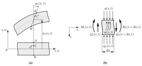
Figure 2. Kinematics and forces/moments in the Timoshenko beam theory. (a) Kinematic assumptions. (b) Infinitesimal element.

In Figure 2b, an infinitesimal element of a Timoshenko beam is shown. The equilibrium of forces and moments leads to

$$\begin{array}{cc}\hfill {\rho }_{\ell }{A}_{\ell }\frac{{\partial }^2{w}_{\ell }(x,t)}{\partial t^2}-\frac{\partial Q_{\ell }(x,t)}{\partial x}-q(x,t)-F_P\left(t\right)\delta (x-X_F)+q_D(x,t)& =0,\hfill \end{array}$$

(13)

$$\begin{array}{cc}\hfill {\rho }_{\ell }{I}_{\ell }\frac{{\partial }^2{\phi }_{\ell }(x,t)}{\partial t^2}-\frac{\partial M_{\ell }(x,t)}{\partial x}+Q_{\ell }(x,t)-m(x,t)-M_P\left(t\right)\delta (x-X_M)& =0,\hfill \end{array}$$

(14)

with $\delta (•)$ the dirac delta function, the external viscous (air) damping

$$q_D(x,t)=d_{a\ell }\frac{\partial w_{\ell }(x,t)}{\partial t},$$

(15)

with $d_{a\ell }>0$ the damping coefficient, the bending moment

$$M_{\ell }(x,t)={\int \int }_A{\sigma }_{xx}(x,z,t)z\mathrm{d}A,$$

(16)

and the shear force

$$Q_{\ell }(x,t)={\int \int }_A{\sigma }_{xz}(x,t)\mathrm{d}A.$$

(17)

For harmonic vibrations at angular frequency $\omega$, the state within a beam segment ℓ is completely described by the transverse displacement ${\tilde{w}}_{\ell }(x,\omega )$, the rotation of the cross-section ${\tilde{\phi }}_{\ell }(x,\omega )$, the bending moment ${\tilde{M}}_{\ell }(x,\omega )$, and the shear force ${\tilde{Q}}_{\ell }(x,\omega )$. Plugging Equations (11) and (12) into Equations (16) and (17) and, subsequently, into Equations (13) and (14) leads to

$$\begin{array}{ll}\frac{{\mathrm{d}}^4{\tilde{w}}_{\ell }\left(x\right)}{\mathrm{d}{x}^4}+\left({\overline{\omega }}_{\ell }^2\left(1+{\overline{E}}_{\ell }\right)-{\overline{d}}_{a\ell }\right)\frac{{\mathrm{d}}^2{\tilde{w}}_{\ell }\left(x\right)}{\mathrm{d}{x}^2}+\hfill & {\overline{\omega }}_{\ell }^2\left({\overline{\omega }}_{\ell }^2{\overline{E}}_{\ell }-\frac{1}{r_{G\ell }^2}-\left(1-\frac{1}{{\overline{E}}_{\ell }{r}_{G\ell }^2{\overline{\omega }}_{\ell }^2}\right){\overline{d}}_{a\ell }\right){\tilde{w}}_{\ell }\left(x\right)=\\ & \hfill \frac{1}{k_{S\ell }{G}_{\ell }^{★}{A}_{\ell }}\left(\left(\frac{1}{{\overline{E}}_{\ell }{r}_{G\ell }^2}-{\overline{\omega }}_{\ell }^2\right)\tilde{q}\left(x\right)-\frac{{\mathrm{d}}^2\tilde{q}\left(x\right)}{\mathrm{d}{x}^2}+\frac{1}{{\overline{E}}_{\ell }{r}_{G\ell }^2}\frac{\mathrm{d}\tilde{m}\left(x\right)}{\mathrm{d}x}\right),\end{array}$$

(18)

$$\begin{array}{cc}\hfill & {\tilde{\phi }}_{\ell }\left(x\right)=\frac{-{\overline{E}}_{\ell }{r}_{G\ell }^2}{1-{\overline{\omega }}_{\ell }^2{\overline{E}}_{\ell }{r}_{G\ell }^2}\left(\frac{{\mathrm{d}}^3{\tilde{w}}_{\ell }\left(x\right)}{\mathrm{d}{x}^3}+\left(\frac{1+{\overline{\omega }}_{\ell }^2{\overline{E}}_{\ell }^2{r}_{G\ell }^2}{{\overline{E}}_{\ell }{r}_{G\ell }^2}-{\overline{d}}_{a\ell }\right)\frac{\mathrm{d}{\tilde{w}}_{\ell }\left(x\right)}{\mathrm{d}x}+\frac{1}{k_{S\ell }{G}_{\ell }^{★}{A}_{\ell }}\left(\frac{\mathrm{d}\tilde{q}\left(x\right)}{\mathrm{d}x}-\frac{\tilde{m}\left(x\right)}{{\overline{E}}_{\ell }{r}_{G\ell }^2}\right)\right),\hfill \end{array}$$

(19)

$$\begin{array}{cc}\hfill & {\tilde{M}}_{\ell }\left(x\right)=E_{\ell }^{★}{I}_{\ell }\frac{\mathrm{d}{\tilde{\phi }}_{\ell }\left(x\right)}{\mathrm{d}x},\hfill \end{array}$$

(20)

$$\begin{array}{cc}\hfill & {\tilde{Q}}_{\ell }\left(x\right)=k_{S\ell }{G}_{\ell }^{★}{A}_{\ell }\left({\tilde{\phi }}_{\ell }\left(x\right)+\frac{\mathrm{d}{\tilde{w}}_{\ell }\left(x\right)}{\mathrm{d}x}\right),\hfill \end{array}$$

(21)

with

$${\overline{\omega }}_{\ell }^2=\frac{{\rho }_{\ell }{\omega }^2}{E_{\ell }^{★}},{\overline{E}}_{\ell }=\frac{E_{\ell }^{★}}{k_{S\ell }{G}_{\ell }^{★}},r_{G\ell }^2=\frac{I_{\ell }}{A_{\ell }},{\overline{d}}_{a\ell }=\frac{\mathrm{j}{d}_{a\ell }\omega }{k_{S\ell }{G}_{\ell }^{★}{A}_{\ell }}$$

(22)

and $k_{S\ell }$ the shear correction factor to account for the actually shear stress distribution. For brevity, the dependency of the variables on $\omega$ in Equations (18)–(21) is dropped, and point loadings are not explicitly stated in the equations but included as special cases of the distributed loadings.

2.4. Boundary and Interface Conditions at the Stations

Since Equation (18) is a fourth order differential equation, four boundary or interface conditions for each segment have to be defined to yield a unique solution. According to Reference [39], the boundary conditions on the left end (station $\left(1\right)$) can be defined by

$$\begin{array}{cccccccccc}{\tilde{w}}_1\left(0\right)& ={\widehat{w}}^{\left(1\right)}& & \mathrm{or}& {\tilde{Q}}_1\left(0\right)& =-{\tilde{F}}_P^{\left(1\right)}& & \mathrm{or}& f_t^{\left(1\right)}({\tilde{w}}_1\left(0\right),{\tilde{Q}}_1\left(0\right))& =0,\end{array}$$

(23)

$$\begin{array}{cccccccccc}\hfill {\tilde{\phi }}_1\left(0\right)& ={\widehat{\phi }}^{\left(1\right)}\hfill & & \mathrm{or}\hfill & \hfill {\tilde{M}}_1\left(0\right)& =-{\tilde{M}}_P^{\left(1\right)}\hfill & & \mathrm{or}\hfill & \hfill f_r^{\left(1\right)}({\tilde{\phi }}_1\left(0\right),{\tilde{M}}_1\left(0\right))& =0,\hfill \end{array}$$

(24)

and on the right end (station $\left(N\right)$) by

$$\begin{array}{cccccccccc}\hfill {\tilde{w}}_M\left(L\right)& ={\widehat{w}}^{\left(N\right)}\hfill & \hfill & \mathrm{or}\hfill & \hfill {\tilde{Q}}_M\left(L\right)& ={\tilde{F}}_P^{\left(N\right)}\hfill & \hfill & \mathrm{or}\hfill & \hfill f_t^{\left(N\right)}({\tilde{w}}_M\left(L\right),{\tilde{Q}}_M\left(L\right))& =0,\hfill \end{array}$$

(25)

$$\begin{array}{cccccccccc}\hfill {\tilde{\phi }}_M\left(L\right)& ={\widehat{\phi }}^{\left(N\right)}\hfill & & \mathrm{or}\hfill & \hfill {\tilde{M}}_M\left(L\right)& ={\tilde{M}}_P^{\left(N\right)}\hfill & & \mathrm{or}\hfill & \hfill f_r^{\left(N\right)}({\tilde{\phi }}_M\left(L\right),{\tilde{M}}_M\left(L\right))& =0,\hfill \end{array}$$

(26)

where ${\widehat{w}}^{\left(1\right)}$ and ${\widehat{w}}^{\left(N\right)}$ are prescribed harmonic displacements, ${\widehat{\phi }}^{\left(1\right)}$ and ${\widehat{\phi }}^{\left(N\right)}$ prescribed harmonic rotations, ${\tilde{F}}_P^{\left(1\right)}$ and ${\tilde{F}}_P^{\left(N\right)}$ prescribed harmonic forces, ${\tilde{M}}_P^{\left(1\right)}$ and ${\tilde{M}}_P^{\left(N\right)}$ prescribed harmonic moments at the left and right boundary, and $f(•,★)$ is a linear function in terms of • and ★, which depends on the concentrated elements at the boundaries.

In case of classical boundary conditions (no concentrated elements at the boundaries), the displacement ${\tilde{w}}_{★}(•)$ or shear force ${\tilde{Q}}_{★}(•)$ and rotation ${\tilde{\phi }}_{★}(•)$ or bending moment ${\tilde{M}}_{★}(•)$ are prescribed. The most common types of classical boundary conditions are the clamped (${\tilde{w}}_{★}(•)=0$, ${\tilde{\phi }}_{★}(•)=0$), free (${\tilde{M}}_{★}(•)=0$, ${\tilde{Q}}_{★}(•)=0$), simply-supported (${\tilde{w}}_{★}(•)=0$, ${\tilde{M}}_{★}(•)=0$), and sliding (${\tilde{\phi }}_{★}(•)=0$, ${\tilde{Q}}_{★}(•)=0$) end conditions.

If concentrated elements are present at the boundaries, a coupling of the displacement and shear force and/or rotation and bending moment appears in the boundary conditions. The forces and moments due to concentrated elements acting on the beam boundaries are shown in Figure 3a,b (station $\left(1\right)$ and station $\left(N\right)$, respectively).

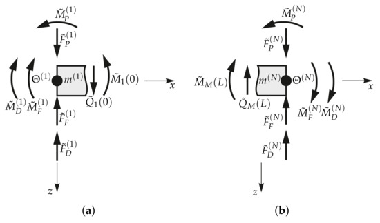
Figure 3. Forces and moments at the left and right boundary. (a) Left boundary. (b) Right boundary.

Using Newton’s second law of motion at the station $\left(1\right)$ leads to

$$\begin{array}{cc}\hfill {\tilde{Q}}_1\left(0\right)+{\tilde{w}}_1\left(0\right)\left(m^{\left(1\right)}{\omega }^2-k_t^{\left(1\right)}-\mathrm{j}\omega d_t^{\left(1\right)}\right)+{\tilde{F}}_P^{\left(1\right)}& =0,\hfill \end{array}$$

(27)

$$\begin{array}{cc}\hfill {\tilde{M}}_1\left(0\right)+{\tilde{\phi }}_1\left(0\right)\left({\mathsf{\Theta }}^{\left(1\right)}{\omega }^2-k_r^{\left(1\right)}-\mathrm{j}\omega d_r^{\left(1\right)}\right)+{\tilde{M}}_P^{\left(1\right)}& =0,\hfill \end{array}$$

(28)

and at station $\left(N\right)$ results in

$$\begin{array}{cc}\hfill {\tilde{Q}}_M\left(L\right)-{\tilde{w}}_M\left(L\right)\left(m^{\left(N\right)}{\omega }^2-k_t^{\left(N\right)}-\mathrm{j}\omega d_t^{\left(N\right)}\right)-{\tilde{F}}_P^{\left(N\right)}& =0,\hfill \end{array}$$

(29)

$$\begin{array}{cc}\hfill {\tilde{M}}_M\left(L\right)-{\tilde{\phi }}_M\left(L\right)\left({\mathsf{\Theta }}^{\left(N\right)}{\omega }^2-k_r^{\left(N\right)}-\mathrm{j}\omega d_r^{\left(N\right)}\right)-{\tilde{M}}_P^{\left(N\right)}& =0,\hfill \end{array}$$

(30)

where ${\tilde{F}}_F^{(•)}=k_t^{(•)}{\tilde{w}}_{★}\left(X_{•}\right)$ (spring force), ${\tilde{F}}_D^{(•)}=\mathrm{j}\omega d_t^{(•)}{\tilde{w}}_{★}\left(X_{•}\right)$ (damping force), ${\tilde{M}}_F^{(•)}=k_r^{(•)}{\tilde{\phi }}_{★}\left(X_{•}\right)$ (spring moment), and ${\tilde{M}}_D^{(•)}=\mathrm{j}\omega d_r^{(•)}{\tilde{\phi }}_{★}\left(X_{•}\right)$ (damping moment) have been applied.

At an intermediate station $\left(i\right)$, the displacement and rotation have to be continuous, which results in

$$\begin{array}{cc}\hfill {\tilde{w}}_{\ell }\left(X_i^{+}\right)-{\tilde{w}}_{\ell -1}\left(X_i^{-}\right)& =0,\hfill \end{array}$$

(31)

$$\begin{array}{cc}\hfill {\tilde{\phi }}_{\ell }\left(X_i^{+}\right)-{\tilde{\phi }}_{\ell -1}\left(X_i^{-}\right)& =0,\hfill \end{array}$$

(32)

where $(i=\ell )$ and $X_i^{-}$ and $X_i^{+}$ are coordinates infinitesimal to the left and right of the station $\left(i\right)$. The forces and moments at an intermediate station $\left(i\right)$ are illustrated in Figure 4.

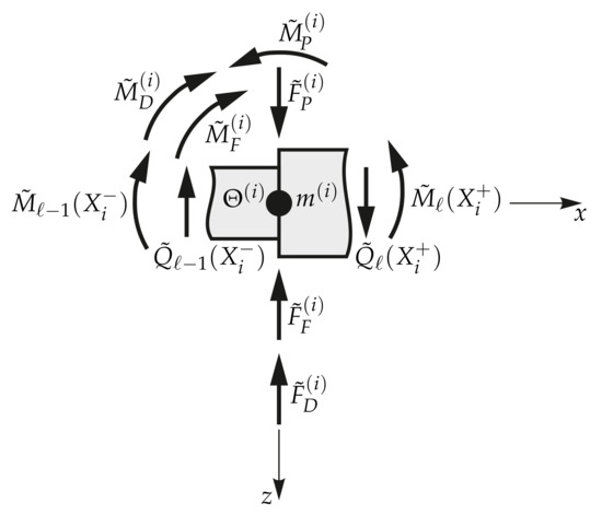
Figure 4. Forces and moments at an intermediate station $\left(i\right)$.

According to Newton’s second law of motion, the equilibrium of forces in z-direction and moments about the y-axis are given by

$$\begin{array}{cc}\hfill {\tilde{Q}}_{\ell }\left(X_i^{+}\right)-{\tilde{Q}}_{\ell -1}\left(X_i^{-}\right)+{\tilde{w}}_{\ell }\left(X_i^{+}\right)\left(m^{\left(i\right)}{\omega }^2-k_t^{\left(i\right)}-\mathrm{j}\omega d_t^{\left(i\right)}\right)+{\tilde{F}}_P^{\left(i\right)}& =0,\hfill \end{array}$$

(33)

$$\begin{array}{cc}\hfill {\tilde{M}}_{\ell }\left(X_i^{+}\right)-{\tilde{M}}_{\ell -1}\left(X_i^{-}\right)+{\tilde{\phi }}_{\ell }\left(X_i^{+}\right)\left({\mathsf{\Theta }}^{\left(i\right)}{\omega }^2-k_r^{\left(i\right)}-\mathrm{j}\omega d_r^{\left(i\right)}\right)+{\tilde{M}}_P^{\left(i\right)}& =0,\hfill \end{array}$$

(34)

with ${\tilde{F}}_P^{\left(i\right)}$ and ${\tilde{M}}_P^{\left(i\right)}$ point loadings, which are directly located at the station $\left(i\right)$.

The harmonic governing equation of an uniform Timoshenko beam given in Equation (18), combined with the boundary conditions in Equations (23)–(30) and the interface conditions in Equations (31)–(34), lead to a well-posed problem.

3. Numerical Assembly Technique

In the Numerical Assembly Technique (NAT), analytical solutions of each beam segment ℓ are used to fulfill the boundary and interface conditions. Since Equation (18) is a linear differential equation, the solution within a beam segment ℓ can be given by ${\tilde{w}}_{\ell }\left(x_{\ell }\right)={\tilde{w}}_{h\ell }\left(x_{\ell }\right)+{\tilde{w}}_{p\ell }\left(x_{\ell }\right)$, with ${\tilde{w}}_{h\ell }\left(x_{\ell }\right)$ and ${\tilde{w}}_{p\ell }\left(x_{\ell }\right)$ as the homogeneous and particular solutions of the governing equation.

3.1. Homogeneous Solution of the Governing Equations

The general homogeneous solution of the harmonic governing equation (Equation (18)) is obtained by setting the external forces and moments to zero ($\tilde{q}\left(x\right)=0$, $\tilde{m}\left(x\right)=0$). Assuming a solution of the form ${\tilde{w}}_{h\ell }\left(x_{\ell }\right)=c_{w\ell }{\mathrm{e}}^{\mathrm{j}k{x}_{\ell }}$, and plugging it into Equation (18), results in the characteristic equation

$$k^4-\left({\overline{\omega }}_{\ell }^2\left(1+{\overline{E}}_{\ell }\right)-{\overline{d}}_{a\ell }\right)k^2+{\overline{\omega }}_{\ell }^2\left({\overline{\omega }}_{\ell }^2{\overline{E}}_{\ell }-\frac{1}{r_{G\ell }^2}-\left(1-\frac{1}{{\overline{E}}_{\ell }{r}_{G\ell }^2{\overline{\omega }}_{\ell }^2}\right){\overline{d}}_{a\ell }\right)=0,$$

(35)

with the solutions

$$\begin{array}{cccc}\hfill k_{1,2}& =\pm \sqrt{\frac{1}{2}\left({\overline{\omega }}_{\ell }^2(1+{\overline{E}}_{\ell })-{\overline{d}}_{a\ell }+R_{\ell }\right)}=\pm {\alpha }_{\ell },\hfill & \hfill \mathrm{Re}\left[{\alpha }_{\ell }\right]>0,& \mathrm{Im}\left[{\alpha }_{\ell }\right]<0,\forall \omega \hfill \end{array}$$

(36)

$$\begin{array}{cccc}\hfill k_{3,4}& =\pm \sqrt{\frac{1}{2}\left({\overline{\omega }}_{\ell }^2(1+{\overline{E}}_{\ell })-{\overline{d}}_{a\ell }-R_{\ell }\right)}=\pm {\beta }_{\ell },\hfill & \hfill \mathrm{Re}\left[{\beta }_{\ell }\right]>0,& \mathrm{Im}\left[{\beta }_{\ell }\right]\left\{\begin{array}{cc}>0,\hfill & \omega \le {\omega }_{c\ell }\hfill \\ <0,\hfill & \omega \ge {\omega }_{c\ell }\hfill \end{array}\right.\hfill \end{array}$$

(37)

and

$$R_{\ell }=\sqrt{{({\overline{E}}_{\ell }-1)}^2{\overline{\omega }}_{\ell }^4+\frac{4{\overline{\omega }}_{\ell }^2}{r_{G\ell }^2}+{\overline{d}}_{a\ell }^2-\frac{4{\overline{d}}_{a\ell }}{{\overline{E}}_{\ell }{r}_{G\ell }^2}-2({\overline{E}}_{\ell }-1){\overline{\omega }}_{\ell }^2{\overline{d}}_{a\ell }}.$$

(38)

At the so-called cut-off angular frequency ${\omega }_{c\ell }$, the characteristic of the third and fourth root changes; therefore, the form of the solutions is also different. For the undamped case, this frequency can be computed analytically, while, for the generally damped case, only a numerical approach is feasible. Using the roots in Equations (36) and (37), the final solutions for the four field-variables are given by

$$\begin{array}{cc}\hfill \underset{{\tilde{\mathbf{x}}}_{h\ell }\left(x_{\ell }\right)}{\underbrace{\left[\begin{array}{c}{\tilde{w}}_{h\ell }\left(x_{\ell }\right)\\ {\tilde{\phi }}_{h\ell }\left(x_{\ell }\right)\\ {\tilde{M}}_{h\ell }\left(x_{\ell }\right)\\ {\tilde{Q}}_{h\ell }\left(x_{\ell }\right)\end{array}\right]}}& =\underset{{\mathbf{B}}_{\ell }\left(x_{\ell }\right)}{\underbrace{\left[\begin{array}{cccc}\hfill {\mathrm{e}}^{\mathrm{j}{\alpha }_{\ell }(x_{\ell }-L_{\ell })}& \hfill {\mathrm{e}}^{-\mathrm{j}{\alpha }_{\ell }{x}_{\ell }}& \hfill {\mathrm{e}}^{\mathrm{j}{\beta }_{\ell }{x}_{\ell }}& \hfill {\mathrm{e}}^{-\mathrm{j}{\beta }_{\ell }(x_{\ell }-L_{\ell })}\\ \hfill -k_{\phi 1\ell }{\mathrm{e}}^{\mathrm{j}{\alpha }_{\ell }(x_{\ell }-L_{\ell })}& \hfill k_{\phi 1\ell }{\mathrm{e}}^{-\mathrm{j}{\alpha }_{\ell }{x}_{\ell }}& \hfill -k_{\phi 2\ell }{\mathrm{e}}^{\mathrm{j}{\beta }_{\ell }{x}_{\ell }}& \hfill k_{\phi 2\ell }{\mathrm{e}}^{-\mathrm{j}{\beta }_{\ell }(x_{\ell }-L_{\ell })}\\ \hfill k_{M1\ell }{\mathrm{e}}^{\mathrm{j}{\alpha }_{\ell }(x_{\ell }-L_{\ell })}& \hfill k_{M1\ell }{\mathrm{e}}^{-\mathrm{j}{\alpha }_{\ell }{x}_{\ell }}& \hfill k_{M2\ell }{\mathrm{e}}^{\mathrm{j}{\beta }_{\ell }{x}_{\ell }}& \hfill k_{M2\ell }{\mathrm{e}}^{-\mathrm{j}{\beta }_{\ell }(x_{\ell }-L_{\ell })}\\ \hfill -k_{Q1\ell }{\mathrm{e}}^{\mathrm{j}{\alpha }_{\ell }(x_{\ell }-L_{\ell })}& \hfill k_{Q1\ell }{\mathrm{e}}^{-\mathrm{j}{\alpha }_{\ell }{x}_{\ell }}& \hfill -k_{Q2\ell }{\mathrm{e}}^{\mathrm{j}{\beta }_{\ell }{x}_{\ell }}& \hfill k_{Q2\ell }{\mathrm{e}}^{-\mathrm{j}{\beta }_{\ell }(x_{\ell }-L_{\ell })}\end{array}\right]}}\underset{{\mathbf{c}}_{\ell }}{\underbrace{\left[\begin{array}{c}{c}_{1\ell }\\ c_{2\ell }\\ c_{3\ell }\\ c_{4\ell }\end{array}\right]}},\omega \le {\omega }_{c\ell },\hfill \end{array}$$

(39)

$$\begin{array}{cc}\hfill \underset{{\tilde{\mathbf{x}}}_{h\ell }\left(x_{\ell }\right)}{\underbrace{\left[\begin{array}{c}{\tilde{w}}_{h\ell }\left(x_{\ell }\right)\\ {\tilde{\phi }}_{h\ell }\left(x_{\ell }\right)\\ {\tilde{M}}_{h\ell }\left(x_{\ell }\right)\\ {\tilde{Q}}_{h\ell }\left(x_{\ell }\right)\end{array}\right]}}& =\underset{{\mathbf{B}}_{\ell }^{*}\left(x_{\ell }\right)}{\underbrace{\left[\begin{array}{cccc}\hfill {\mathrm{e}}^{\mathrm{j}{\alpha }_{\ell }(x_{\ell }-L_{\ell })}& \hfill {\mathrm{e}}^{-\mathrm{j}{\alpha }_{\ell }{x}_{\ell }}& \hfill {\mathrm{e}}^{\mathrm{j}{\beta }_{\ell }(x_{\ell }-L_{\ell })}& \hfill {\mathrm{e}}^{-\mathrm{j}{\beta }_{\ell }{x}_{\ell }}\\ \hfill -k_{\phi 1\ell }{\mathrm{e}}^{\mathrm{j}{\alpha }_{\ell }(x_{\ell }-L_{\ell })}& \hfill k_{\phi 1\ell }{\mathrm{e}}^{-\mathrm{j}{\alpha }_{\ell }{x}_{\ell }}& \hfill -k_{\phi 2\ell }{\mathrm{e}}^{\mathrm{j}{\beta }_{\ell }(x_{\ell }-L_{\ell })}& \hfill k_{\phi 2\ell }{\mathrm{e}}^{-\mathrm{j}{\beta }_{\ell }{x}_{\ell }}\\ \hfill k_{M1\ell }{\mathrm{e}}^{\mathrm{j}{\alpha }_{\ell }(x_{\ell }-L_{\ell })}& \hfill k_{M1\ell }{\mathrm{e}}^{-\mathrm{j}{\alpha }_{\ell }{x}_{\ell }}& \hfill k_{M2\ell }{\mathrm{e}}^{\mathrm{j}{\beta }_{\ell }(x_{\ell }-L_{\ell })}& \hfill k_{M2\ell }{\mathrm{e}}^{-\mathrm{j}{\beta }_{\ell }{x}_{\ell }}\\ \hfill -k_{Q1\ell }{\mathrm{e}}^{\mathrm{j}{\alpha }_{\ell }(x_{\ell }-L_{\ell })}& \hfill k_{Q1\ell }{\mathrm{e}}^{-\mathrm{j}{\alpha }_{\ell }{x}_{\ell }}& \hfill -k_{Q2\ell }{\mathrm{e}}^{\mathrm{j}{\beta }_{\ell }(x_{\ell }-L_{\ell })}& \hfill k_{Q2\ell }{\mathrm{e}}^{-\mathrm{j}{\beta }_{\ell }{x}_{\ell }}\end{array}\right]}}\underset{{\mathbf{c}}_{\ell }^{*}}{\underbrace{\left[\begin{array}{c}{c}_{1\ell }\\ c_{2\ell }\\ c_{3\ell }^{*}\\ c_{4\ell }^{*}\end{array}\right]}},\omega \ge {\omega }_{c\ell },\hfill \end{array}$$

(40)

with the constants

$$\begin{array}{cccc}\hfill k_{\phi 1\ell }& =\frac{\mathrm{j}\left({\alpha }_{\ell }^2-{\overline{E}}_{\ell }{\overline{\omega }}_{\ell }^2+{\overline{d}}_{a\ell }\right)}{{\alpha }_{\ell }},\hfill & \hfill k_{\phi 2\ell }& =\frac{\mathrm{j}\left({\beta }_{\ell }^2-{\overline{E}}_{\ell }{\overline{\omega }}_{\ell }^2+{\overline{d}}_{a\ell }\right)}{{\beta }_{\ell }},\hfill \end{array}$$

(41)

$$\begin{array}{cccc}\hfill k_{M1\ell }& =E_{\ell }^{★}{I}_{\ell }\left({\alpha }_{\ell }^2-{\overline{E}}_{\ell }{\overline{\omega }}_{\ell }^2+{\overline{d}}_{a\ell }\right),\hfill & \hfill k_{M2\ell }& =E_{\ell }^{★}{I}_{\ell }\left({\beta }_{\ell }^2-{\overline{E}}_{\ell }{\overline{\omega }}_{\ell }^2+{\overline{d}}_{a\ell }\right),\hfill \end{array}$$

(42)

$$\begin{array}{cccc}\hfill k_{Q1\ell }& =\mathrm{j}{k}_{S\ell }{G}_{\ell }^{★}{A}_{\ell }\frac{-{\overline{E}}_{\ell }{\overline{\omega }}_{\ell }^2+{\overline{d}}_{a\ell }}{{\alpha }_{\ell }},\hfill & \hfill k_{Q2\ell }& =\mathrm{j}{k}_{S\ell }{G}_{\ell }^{★}{A}_{\ell }\frac{-{\overline{E}}_{\ell }{\overline{\omega }}_{\ell }^2+{\overline{d}}_{a\ell }}{{\beta }_{\ell }}.\hfill \end{array}$$

(43)

In Equations (39) and (40), the field variables are gathered in the column vector ${\tilde{\mathbf{x}}}_{h\ell }\left(x_{\ell }\right)$ and the arbitrary constants $c_{•}$ in the column vectors ${\mathbf{c}}_{\ell }$ and ${\mathbf{c}}_{\ell }^{*}$. The state variable matrices ${\mathit{B}}_{\ell }\left(x_{\ell }\right)$ and ${{B}}_{\ell }^{*}\left(x_{\ell }\right)$ below and above the cut-off frequency are slightly different, since the entries in the matrices are scaled to unity within the segment length ($x_{\ell }=[0,L_{\ell }]$). This scaling has certain numerical advantages, since the terms with positive real parts in the exponents would grow very rapidly and lead to a bad conditioning of the resulting system matrices. In Section 3.3, the boundary and interface conditions are used to calculate the arbitrary constants $c_{•}$.

3.2. Particular Solutions of the Governing Equations

The particular solutions of the governing equation ${\tilde{w}}_{p\ell }\left(x_{\ell }\right)$ fulfill the right-hand side of Equation (18). Depending on the type of loading, different solution procedures are necessary. In case of concentrated loadings, the Fourier transform [40] and the residue theorem and Jordan’s Lemma [41] are applied to calculated the particular solutions. For generally distributed loadings, a two-step approach is required. First, the loading functions are approximated by a Fourier extension (continuation) method [33], and then the Green’s function method [42] is used to compute the particular solutions. In the subsequent sections, an overview of the applied mathematical principle is given, and the particular solutions for point loadings and generally distributed loadings are derived.

3.2.1. Fourier Transform, Residue Theorem, and Jordan’s Lemma

The Fourier transform is well suited to solve inhomogeneous differential equations, due to its operational property for derivatives [40]

$$\mathcal{F}\left\{\frac{{\mathrm{d}}^{n}g\left(x\right)}{\mathrm{d}{x}^n}\right\}={\left(\mathrm{j}k\right)}^n\widehat{g}\left(k\right),$$

(44)

where $\widehat{g}\left(k\right)$ is the spatial Fourier transform $\mathcal{F}\{•\}$ of the function $g\left(x\right)$ and $n\in {\mathbb{N}}_0$.

The inverse Fourier transform ${\mathcal{F}}^{-1}\{•\}$ involves the evaluation of integrals on the real axis ranging from $-\infty$ to ∞. A powerful tool to evaluate such integrals is the residue theorem [41]. The residue theorem leads to the integral formulas [41]

$$\underset{-\infty }{\overset{\infty }{\int }}\widehat{g}\left(k\right){\mathrm{e}}^{\mathrm{j}kx}\mathrm{d}k=\left\{\begin{array}{cc}{\displaystyle \phantom{-}2\pi \mathrm{j}\sum _{i=1}^{s^{+}}\underset{z=z_i^{+}}{\mathrm{Res}}\left\{\widehat{g}\left(z\right){\mathrm{e}}^{\mathrm{j}zx}\right\}+\pi \mathrm{j}\sum _{i=1}^m\underset{z=p_i}{\mathrm{Res}}\left\{\widehat{g}\left(z\right){\mathrm{e}}^{\mathrm{j}zx}\right\}}\hfill & x>0,\hfill \\ {\displaystyle -2\pi \mathrm{j}\sum _{i=1}^{s^{-}}\underset{z=z_i^{-}}{\mathrm{Res}}\left\{\widehat{g}\left(z\right){\mathrm{e}}^{\mathrm{j}zx}\right\}-\pi \mathrm{j}\sum _{i=1}^m\underset{z=p_i}{\mathrm{Res}}\left\{\widehat{g}\left(z\right){\mathrm{e}}^{\mathrm{j}zx}\right\}}\hfill & x<0,\hfill \end{array}\right.$$

(45)

where $z_i^{+}$ are poles in the upper half plane (total number $s^{+}$), $z_i^{-}$ poles in the lower half plane (total number $s^{-}$), $p_i$ poles on the real axis (total number m), and $\mathrm{Res}\{•\}$ is the residue at the pole. The integral formulas in Equation (45) are only valid if Jordan’s Lemma is applicable, which requires the condition

$$\underset{\left|z\right|\to \infty }{lim}\widehat{g}\left(z\right)=0,$$

(46)

with $|•|$ the absolute value [41]. Several methods are available to evaluate the residues. Since only simple poles appear in the following calculations, the formula [41]

$$\underset{z=z_i}{\mathrm{Res}}\left\{\widehat{g}\left(z\right){\mathrm{e}}^{\mathrm{j}zx}\right\}=\underset{z\to z_i}{lim}(z-z_i)\widehat{g}\left(z\right){\mathrm{e}}^{\mathrm{j}zx}$$

(47)

can be applied, which is valid for simple poles $z_i\ne \infty$.

3.2.2. Concentrated Loads

Using a Fourier transform of Equation (18) with respect to the spatial coordinate $x_{\ell }$, the displacement of the beam segment ℓ in the transformed domain is given by

$${\widehat{w}}_{p\ell }\left(k\right)=\frac{1}{k_{S\ell }{G}_{\ell }^{★}{A}_{\ell }}\frac{\left(k^2+\frac{1}{{\overline{E}}_{\ell }{r}_{G\ell }^2}-{\overline{\omega }}_{\ell }^2\right)\widehat{q}\left(k\right)+\frac{\mathrm{j}k}{{\overline{E}}_{\ell }{r}_{G\ell }^2}\widehat{m}\left(k\right)}{(k-{\alpha }_{\ell })(k+{\alpha }_{\ell })(k-{\beta }_{\ell })(k+{\beta }_{\ell })},$$

(48)

with ${\widehat{w}}_{p\ell }\left(k\right)$, $\widehat{q}\left(k\right)$, and $\widehat{m}\left(k\right)$ as the spatial Fourier transforms of ${\tilde{w}}_{p\ell }\left(x\right)$, $\tilde{q}\left(x\right)$, and $\tilde{m}\left(x\right)$. The inverse Fourier transform leads to the particular solution in an integral form

$${\tilde{w}}_{p\ell }\left(x_{\ell }\right)=\frac{1}{2\pi }\underset{-\infty }{\overset{\infty }{\int }}{\widehat{w}}_{p\ell }\left(k\right){\mathrm{e}}^{\mathrm{j}k{x}_{\ell }}\mathrm{d}k,$$

(49)

which can be analytically evaluated for concentrated loadings.

Point Force

A point force with the amplitude ${\tilde{F}}_P$ acting at the coordinate $x_{\ell }=X_F$ is given by

$$\tilde{q}\left(x_{\ell }\right)={\tilde{F}}_P\delta (x_{\ell }-X_F),$$

(50)

with $\delta (•)$ the dirac delta function. The Fourier transform of the point force is given by

$$\widehat{q}\left(k\right)={\tilde{F}}_P{\mathrm{e}}^{-\mathrm{j}k{X}_F}.$$

(51)

Plugging the Fourier transform of the point force into Equations (48) and (49) leads to the displacement

$${\tilde{w}}_{p\ell }\left(x_{\ell }\right)=\frac{{\tilde{F}}_P}{2\pi k_{S\ell }{G}_{\ell }^{★}{A}_{\ell }}\underset{-\infty }{\overset{\infty }{\int }}\frac{k^2+\frac{1}{{\overline{E}}_{\ell }{r}_{G\ell }^2}-{\overline{\omega }}_{\ell }^2}{(k-{\alpha }_{\ell })(k+{\alpha }_{\ell })(k-{\beta }_{\ell })(k+{\beta }_{\ell })}{\mathrm{e}}^{\mathrm{j}k(x_{\ell }-X_F)}\mathrm{d}k,$$

(52)

and the evaluation of the integral with the residue theorem results in

$$\begin{array}{c}\hfill {\tilde{w}}_{p\ell }\left(x_{\ell }\right)=-\frac{\mathrm{j}{\tilde{F}}_P}{2E_{\ell }^{★}{I}_{\ell }\left({\alpha }_{\ell }^2-{\beta }_{\ell }^2\right)}\left(\frac{1+{\overline{E}}_{\ell }{r}_{G\ell }^2\left({\alpha }_{\ell }^2-{\overline{\omega }}_{\ell }^2\right)}{{\alpha }_{\ell }}{\mathrm{e}}^{-\mathrm{j}{\alpha }_{\ell }|x_{\ell }-X_F|}\pm \frac{1+{\overline{E}}_{\ell }{r}_{G\ell }^2\left({\beta }_{\ell }^2-{\overline{\omega }}_{\ell }^2\right)}{{\beta }_{\ell }}{\mathrm{e}}^{\pm \mathrm{j}{\beta }_{\ell }|x_{\ell }-X_F|}\right).\end{array}$$

(53)

Due to the characteristic change of ${\beta }_{\ell }$ at the cut-off frequency ${\omega }_{c\ell }$, two different cases have to be considered. The upper signs in Equation (53) belong to $\omega \le {\omega }_{c\ell }$, and the lower signs to $\omega \ge {\omega }_{c\ell }$. This compact representation of the two cases is adopted in all following equations. The remaining field variables are computed by Equations (19)–(21) and are given by

$$\begin{array}{cc}\hfill {\tilde{\phi }}_{p\ell }\left(x_{\ell }\right)& =\frac{{\tilde{F}}_P\mathrm{sgn}(x_{\ell }-X_F)}{2E_{\ell }^{★}{I}_{\ell }\left({\alpha }_{\ell }^2-{\beta }_{\ell }^2\right)}\left({\mathrm{e}}^{-\mathrm{j}{\alpha }_{\ell }|x_{\ell }-X_F|}-{\mathrm{e}}^{\pm \mathrm{j}{\beta }_{\ell }|x_{\ell }-X_F|}\right),\hfill \end{array}$$

(54)

$$\begin{array}{cc}\hfill {\tilde{M}}_{p\ell }\left(x_{\ell }\right)& =-\frac{\mathrm{j}{\tilde{F}}_P}{2\left({\alpha }_{\ell }^2-{\beta }_{\ell }^2\right)}\left({\alpha }_{\ell }{\mathrm{e}}^{-\mathrm{j}{\alpha }_{\ell }|x_{\ell }-X_F|}\pm {\beta }_{\ell }{\mathrm{e}}^{\pm \mathrm{j}{\beta }_{\ell }|x_{\ell }-X_F|}\right),\hfill \end{array}$$

(55)

$$\begin{array}{cc}\hfill {\tilde{Q}}_{p\ell }\left(x_{\ell }\right)& =-\frac{{\tilde{F}}_P\mathrm{sgn}(x_{\ell }-X_F)}{2\left({\alpha }_{\ell }^2-{\beta }_{\ell }^2\right)}\left(\left({\alpha }_{\ell }^2-{\overline{\omega }}_{\ell }^2\right){\mathrm{e}}^{-\mathrm{j}{\alpha }_{\ell }|x_{\ell }-X_F|}-\left({\beta }_{\ell }^2-{\overline{\omega }}_{\ell }^2\right){\mathrm{e}}^{\pm \mathrm{j}{\beta }_{\ell }|x_{\ell }-X_F|}\right),\hfill \end{array}$$

(56)

with $\mathrm{sgn}(•)$ the signum function. The particular solutions of the field variables are gathered in the column vector ${\tilde{\mathbf{x}}}_{p\ell }={[{\tilde{w}}_{p\ell }\left(x_{\ell }\right),{\tilde{\phi }}_{p\ell }\left(x_{\ell }\right),{\tilde{M}}_{p\ell }\left(x_{\ell }\right),{\tilde{Q}}_{p\ell }\left(x_{\ell }\right)]}^T$.

Point Moment

The procedure for the derivation of the particular solutions due to a point moment is completely equal to the point force. For completeness, the solutions of the field variables are stated

$$\begin{array}{cc}\hfill {\tilde{w}}_{p\ell }\left(x_{\ell }\right)& =-\frac{{\tilde{M}}_P\mathrm{sgn}(x_{\ell }-X_M)}{2E_{\ell }^{★}{I}_{\ell }\left({\alpha }_{\ell }^2-{\beta }_{\ell }^2\right)}\left({\mathrm{e}}^{-\mathrm{j}{\alpha }_{\ell }|x_{\ell }-X_M|}-{\mathrm{e}}^{\pm \mathrm{j}{\beta }_{\ell }|x_{\ell }-X_M|}\right),\hfill \end{array}$$

(57)

$$\begin{array}{cc}\hfill {\tilde{\phi }}_{p\ell }\left(x_{\ell }\right)& =\frac{\mathrm{j}{\tilde{M}}_P}{2E_{\ell }^{★}{I}_{\ell }\left({\alpha }_{\ell }^2-{\beta }_{\ell }^2\right)}\left(\frac{{\beta }_{\ell }^2-{\overline{\omega }}_{\ell }^2}{{\alpha }_{\ell }}{\mathrm{e}}^{-\mathrm{j}{\alpha }_{\ell }|x_{\ell }-X_M|}\pm \frac{{\alpha }_{\ell }^2-{\overline{\omega }}_{\ell }^2}{{\beta }_{\ell }}{\mathrm{e}}^{\pm \mathrm{j}{\beta }_{\ell }|x_{\ell }-X_M|}\right),\hfill \end{array}$$

(58)

$$\begin{array}{cc}\hfill {\tilde{M}}_{p\ell }\left(x_{\ell }\right)& =\frac{{\tilde{M}}_P\mathrm{sgn}(x_{\ell }-X_M)}{2\left({\alpha }_{\ell }^2-{\beta }_{\ell }^2\right)}\left(\left({\beta }_{\ell }^2-{\overline{\omega }}_{\ell }^2\right){\mathrm{e}}^{-\mathrm{j}{\alpha }_{\ell }|x_{\ell }-X_M|}-\left({\alpha }_{\ell }^2-{\overline{\omega }}_{\ell }^2\right){\mathrm{e}}^{\pm \mathrm{j}{\beta }_{\ell }|x_{\ell }-X_M|}\right),\hfill \end{array}$$

(59)

$$\begin{array}{cc}\hfill {\tilde{Q}}_{p\ell }\left(x_{\ell }\right)& =\frac{\mathrm{j}{\tilde{M}}_P\left({\overline{E}}_{\ell }{\overline{\omega }}_{\ell }^2-{\overline{d}}_{a\ell }\right)}{2{\overline{E}}_{\ell }{r}_{G\ell }^2\left({\alpha }_{\ell }^2-{\beta }_{\ell }^2\right)}\left(\frac{1}{{\alpha }_{\ell }}{\mathrm{e}}^{-\mathrm{j}{\alpha }_{\ell }|x_{\ell }-X_M|}\pm \frac{1}{{\beta }_{\ell }}{\mathrm{e}}^{\pm \mathrm{j}{\beta }_{\ell }|x_{\ell }-X_M|}\right).\hfill \end{array}$$

(60)

3.2.3. Generally Distributed Loads

The particular solution functions for distributed loads are derived using the Green’s function method, which uses the response due to a unit point source (Green’s function) and an integration over the distributed load region [42]. In Figure 5a,b, the limits and coordinate systems used for distributed forces and moments are shown.

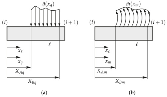
Figure 5. Limits and coordinate systems of the distributed loads. (a) Distributed force. (b) Distributed moment.

Setting the point loads ${\tilde{F}}_P$ and ${\tilde{M}}_P$ in Equations (53) and (57) to one, multiplying the solutions with the distributed loadings $\tilde{q}\left(x_q\right)$ and $\tilde{m}\left(x_m\right)$, and integrating over the load region lead to the particular solutions

$$\begin{array}{cc}\hfill {\tilde{w}}_{p\ell }\left(x_{\ell }\right)& =-\frac{\mathrm{j}}{2E_{\ell }^{★}{I}_{\ell }\left({\alpha }_{\ell }^2-{\beta }_{\ell }^2\right)}\underset{X_{Aq}}{\overset{X_{Bq}}{\int }}\tilde{q}\left(x_q\right)\left(\frac{1+{\overline{E}}_{\ell }{r}_{G\ell }^2\left({\alpha }_{\ell }^2-{\overline{\omega }}_{\ell }^2\right)}{{\alpha }_{\ell }}{\mathrm{e}}^{-\mathrm{j}{\alpha }_{\ell }|x_{\ell }-x_q|}\pm \frac{1+{\overline{E}}_{\ell }{r}_{G\ell }^2\left({\beta }_{\ell }^2-{\overline{\omega }}_{\ell }^2\right)}{{\beta }_{\ell }}{\mathrm{e}}^{\pm \mathrm{j}{\beta }_{\ell }|x_{\ell }-x_q|}\right)\mathrm{d}{x}_q,\hfill \end{array}$$

(61)

$$\begin{array}{cc}\hfill {\tilde{w}}_{p\ell }\left(x_{\ell }\right)& =-\frac{1}{2E_{\ell }^{★}{I}_{\ell }\left({\alpha }_{\ell }^2-{\beta }_{\ell }^2\right)}\underset{X_{Am}}{\overset{X_{Bm}}{\int }}\tilde{m}\left(x_m\right)\mathrm{sgn}(x_{\ell }-x_m)\left({\mathrm{e}}^{-\mathrm{j}{\alpha }_{\ell }|x_{\ell }-x_m|}-{\mathrm{e}}^{\pm \mathrm{j}{\beta }_{\ell }|x_{\ell }-x_m|}\right)\mathrm{d}{x}_m,\hfill \end{array}$$

(62)

which are given in a general integral form. Applying a change of variables to normalized local coordinates with respect to the limits of the distributed loading

$${\overline{x}}_{•}=\left(x_{•}-\frac{X_{B•}+X_{A•}}{2}\right)\frac{2}{X_{B•}-X_{A•}}$$

(63)

and

$${\overline{x}}_{\ell }=\left(x_{\ell }-\frac{X_{B•}+X_{A•}}{2}\right)\frac{2}{X_{B•}-X_{A•}}$$

(64)

simplifies Equations (61) and (62) to

$$\begin{array}{cc}\hfill {\tilde{w}}_{p\ell }\left({\overline{x}}_{\ell }\right)& =-\frac{\mathrm{j}{\left(X_{Bq}-X_{Aq}\right)}^4}{32E_{\ell }^{★}{I}_{\ell }\left({\overline{\alpha }}_{\ell }^2-{\overline{\beta }}_{\ell }^2\right)}\underset{-1}{\overset{1}{\int }}\tilde{q}\left({\overline{x}}_q\right)\left(\frac{1+{\overline{E}}_{\ell }{r}_{G\ell }^2\left({\alpha }_{\ell }^2-{\overline{\omega }}_{\ell }^2\right)}{{\overline{\alpha }}_{\ell }}{\mathrm{e}}^{-\mathrm{j}{\overline{\alpha }}_{\ell }|{\overline{x}}_{\ell }-{\overline{x}}_q|}\pm \frac{1+{\overline{E}}_{\ell }{r}_{G\ell }^2\left({\beta }_{\ell }^2-{\overline{\omega }}_{\ell }^2\right)}{{\overline{\beta }}_{\ell }}{\mathrm{e}}^{\pm \mathrm{j}{\overline{\beta }}_{\ell }|{\overline{x}}_{\ell }-{\overline{x}}_q|}\right)\mathrm{d}{\overline{x}}_q,\hfill \end{array}$$

(65)

$$\begin{array}{cc}\hfill {\tilde{w}}_{p\ell }\left({\overline{x}}_{\ell }\right)& =-\frac{{\left(X_{Bm}-X_{Am}\right)}^3}{16E_{\ell }^{★}{I}_{\ell }\left({\overline{\alpha }}_{\ell }^2-{\overline{\beta }}_{\ell }^2\right)}\underset{-1}{\overset{1}{\int }}\tilde{m}\left({\overline{x}}_m\right)\mathrm{sgn}({\overline{x}}_{\ell }-{\overline{x}}_m)\left({\mathrm{e}}^{-\mathrm{j}{\overline{\alpha }}_{\ell }|{\overline{x}}_{\ell }-{\overline{x}}_m|}-{\mathrm{e}}^{\pm \mathrm{j}{\overline{\beta }}_{\ell }|{\overline{x}}_{\ell }-{\overline{x}}_m|}\right)\mathrm{d}{\overline{x}}_m,\hfill \end{array}$$

(66)

with

$$\begin{array}{cc}\hfill {\overline{\alpha }}_{\ell }& ={\alpha }_{\ell }\frac{X_{B•}-X_{A•}}{2},\hfill \end{array}$$

(67)

$$\begin{array}{cc}\hfill {\overline{\beta }}_{\ell }& ={\beta }_{\ell }\frac{X_{B•}-X_{A•}}{2},\hfill \end{array}$$

(68)

normalized angular wavenumbers.

Generally Distributed Force

Since the evaluation of the integral in Equation (65) strongly depends on the actual distribution of the excitation and has to be performed for any problem specific function individually, a different approach is taken. An approximation of the distributed force with the so-called Fourier extension (continuation) method is applied to allow for a systematic procedure to compute the particular solution for any given force distribution. In the Fourier extension method, a non-periodic function, which is defined on the interval $[-1,1]$, is approximated by a Fourier series that is periodic on an extended interval $[-T,T]$$(T>1)$[43,44]. Therefore, the generally distributed force, given in normalized local coordinates ${\overline{x}}_q$, is approximated by the Fourier series

$$\tilde{q}\left({\overline{x}}_q\right)\approx \frac{1}{\sqrt{2T}}\sum _{k=-n}^n{d}_{qk}{\mathrm{e}}^{\mathrm{j}\frac{k\pi }{T}{\overline{x}}_q}\mathrm{with}-1\le {\overline{x}}_q\le 1,$$

(69)

with $T>1$ and n corresponding to the order of the approximation. A very efficient way to calculate the complex coefficients $d_{qk}$ is presented by Adcock and Huybrechs [43], which is called the numerical discrete Fourier extension with equispaced sampling points. Efficient and stable numerical algorithms of this method are developed in References [44,45]. A detailed description of the algorithm, which is applied in this paper, can be found in Reference [44], and additional information on the convergency rate and stability of the Fourier extension method is given in, e.g., References [43,46].

Plugging the Fourier extension of the distributed force (Equation (69)) into Equation (65), and analytically evaluating the integrals, leads to the particular solution

$${\tilde{w}}_{p\ell }\left({\overline{x}}_{\ell }\right)=\sum _{k=-n}^n-\frac{\mathrm{j}{d}_{qk}{(X_{Bq}-X_{Aq})}^4}{32E_{\ell }^{★}{I}_{\ell }\left({\overline{\alpha }}_{\ell }^2-{\overline{\beta }}_{\ell }^2\right)}\left(\frac{1+{\overline{E}}_{\ell }{r}_{G\ell }^2\left({\alpha }_{\ell }^2-{\overline{\omega }}_{\ell }^2\right)}{{\overline{\alpha }}_{\ell }}{I}_1({\overline{x}}_{\ell },k)\pm \frac{1+{\overline{E}}_{\ell }{r}_{G\ell }^2\left({\beta }_{\ell }^2-{\overline{\omega }}_{\ell }^2\right)}{{\overline{\beta }}_{\ell }}{I}_3({\overline{x}}_{\ell },k)\right),$$

(70)

with the integrals $I_1({\overline{x}}_{\ell },k)$ and $I_3({\overline{x}}_{\ell },k)$ presented in Appendix A. The remaining field variables can either be computed by an integration of the point solutions (Equations (54)–(56)) or by applying Equations (19)–(21). The results for the rotation, bending moment, and shear force are given by

$$\begin{array}{cc}\hfill {\tilde{\phi }}_{p\ell }\left({\overline{x}}_{\ell }\right)& =\sum _{k=-n}^n\frac{d_{qk}{(X_{Bq}-X_{Aq})}^3}{16E_{\ell }^{★}{I}_{\ell }\left({\overline{\alpha }}_{\ell }^2-{\overline{\beta }}_{\ell }^2\right)}\left(I_2({\overline{x}}_{\ell },k)-I_4({\overline{x}}_{\ell },k)\right),\hfill \end{array}$$

(71)

$$\begin{array}{cc}\hfill {\tilde{M}}_{p\ell }\left({\overline{x}}_{\ell }\right)& =\sum _{k=-n}^n-\frac{\mathrm{j}{d}_{qk}{(X_{Bq}-X_{Aq})}^2}{8\left({\overline{\alpha }}_{\ell }^2-{\overline{\beta }}_{\ell }^2\right)}\left({\overline{\alpha }}_{\ell }{I}_1({\overline{x}}_{\ell },k)\pm {\overline{\beta }}_{\ell }{I}_3({\overline{x}}_{\ell },k)\right),\hfill \end{array}$$

(72)

$$\begin{array}{cc}\hfill {\tilde{Q}}_{p\ell }\left({\overline{x}}_{\ell }\right)& =\sum _{k=-n}^n-\frac{d_{qk}{(X_{Bq}-X_{Aq})}^3}{16\left({\overline{\alpha }}_{\ell }^2-{\overline{\beta }}_{\ell }^2\right)}\left(\left({\alpha }_{\ell }^2-{\overline{\omega }}_{\ell }^2\right)I_2({\overline{x}}_{\ell },k)-\left({\beta }_{\ell }^2-{\overline{\omega }}_{\ell }^2\right)I_4({\overline{x}}_{\ell },k)\right),\hfill \end{array}$$

(73)

where the integrals $I_2({\overline{x}}_{\ell },k)$ and $I_4({\overline{x}}_{\ell },k)$ are also presented in Appendix A. The particular solutions for a generally distributed force are only quasi-analytical, since a small approximation error remains due to the Fourier extension method. This error can even be reduced to double-precision accuracy if the order n of the Fourier extension is high enough.

Generally Distributed Moment

The calculation of the particular solutions due to a generally distributed moment is completely equivalent. The distributed moment is approximated by a Fourier series

$$\tilde{m}\left({\overline{x}}_m\right)\approx \frac{1}{\sqrt{2T}}\sum _{k=-n}^n{d}_{mk}{\mathrm{e}}^{\mathrm{j}\frac{k\pi }{T}{\overline{x}}_m}\mathrm{with}-1\le {\overline{x}}_m\le 1,$$

(74)

and evaluating the resulting integrals in Equation (66) leads to

$$\begin{array}{cc}\hfill {\tilde{w}}_{p\ell }\left({\overline{x}}_{\ell }\right)& =\sum _{k=-n}^n-\frac{d_{mk}{\left(X_{Bm}-X_{Am}\right)}^3}{16E_{\ell }^{★}{I}_{\ell }\left({\overline{\alpha }}_{\ell }^2-{\overline{\beta }}_{\ell }^2\right)}\left(I_2({\overline{x}}_{\ell },k)-I_4({\overline{x}}_{\ell },k)\right),\hfill \end{array}$$

(75)

$$\begin{array}{cc}\hfill {\tilde{\phi }}_{p\ell }\left({\overline{x}}_{\ell }\right)& =\sum _{k=-n}^n\frac{\mathrm{j}{d}_{mk}{\left(X_{Bm}-X_{Am}\right)}^4}{32E_{\ell }^{★}{I}_{\ell }\left({\overline{\alpha }}_{\ell }^2-{\overline{\beta }}_{\ell }^2\right)}\left(\frac{{\beta }_{\ell }^2-{\overline{\omega }}_{\ell }^2}{{\overline{\alpha }}_{\ell }}{I}_1({\overline{x}}_{\ell },k)\pm \frac{{\alpha }_{\ell }^2-{\overline{\omega }}_{\ell }^2}{{\overline{\beta }}_{\ell }}{I}_3({\overline{x}}_{\ell },k)\right),\hfill \end{array}$$

(76)

$$\begin{array}{cc}\hfill {\tilde{M}}_{p\ell }\left({\overline{x}}_{\ell }\right)& =\sum _{k=-n}^n\frac{d_{mk}{\left(X_{Bm}-X_{Am}\right)}^3}{16\left({\overline{\alpha }}_{\ell }^2-{\overline{\beta }}_{\ell }^2\right)}\left(\left({\beta }_{\ell }^2-{\overline{\omega }}_{\ell }^2\right)I_2({\overline{x}}_{\ell },k)-\left({\alpha }_{\ell }^2-{\overline{\omega }}_{\ell }^2\right)I_4({\overline{x}}_{\ell },k)\right),\hfill \end{array}$$

(77)

$$\begin{array}{cc}\hfill {\tilde{Q}}_{p\ell }\left({\overline{x}}_{\ell }\right)& =\sum _{k=-n}^n\frac{\mathrm{j}{d}_{mk}{\left(X_{Bm}-X_{Am}\right)}^4\left({\overline{E}}_{\ell }{\overline{\omega }}_{\ell }^2-{\overline{d}}_{a\ell }\right)}{32{\overline{E}}_{\ell }{r}_{G\ell }^2\left({\overline{\alpha }}_{\ell }^2-{\overline{\beta }}_{\ell }^2\right)}\left(\frac{1}{{\overline{\alpha }}_{\ell }}{I}_1({\overline{x}}_{\ell },k)\pm \frac{1}{{\overline{\beta }}_{\ell }}{I}_3({\overline{x}}_{\ell },k)\right).\hfill \end{array}$$

(78)

3.3. Assembly Procedure and Solution Process

The homogeneous and particular solutions, derived in Section 3.1 and Section 3.2, are used to fulfill the boundary and interface conditions stated in Equations (23)–(34). This procedure leads to a system of linear equations of the form $\mathit{A}\mathit{c}=\mathit{b}$, with the $4M\times 4M$ system matrix $\mathit{A}$ and the $4M\times 1$ right-hand side vector b. The arbitrary constants ${\mathit{c}}_{\ell }$ of each segment are gathered in the $4M\times 1$ vector $\mathit{c}$. Solving the system of linear equations for $\mathit{c}$ results in a quasi-analytical solution of the beam vibration problem stated in Section 2.1. A detailed description of the assembly procedure can be found in the authors’ previous paper [27].

4. Numerical and Experimental Validation Examples

In the following sections, numerical and experimental validation examples are presented. In Section 4.1, a general beam system is investigated using NAT and FEM, and the numerical solutions are compared with respect to accuracy and computational efficiency. Additionally, the behavior of different viscoelastic material models is examined. A validation of NAT and the fractional Zener material model with measurement data is shown in Section 4.2. Two different test setups with materials having low (steel) and high (PVC) internal damping are used to show the broad applicability of the fractional Zener model and the presented numerical technique.

All computations are performed on an Intel^® Xeon^® E3-1270 processor ($4\times 3.6\mathrm{GHz}$) with $32\mathrm{GB}$ RAM and a Windows 10 operating system. The software package MATLAB^®$R2020\mathrm{b}$ is used to implement NAT, while the FEM models are built in the commercial software Abaqus FEA^® 2017.

4.1. Numerical Validation Example

In Figure 6, a multiple-stepped beam with circular cross-sections including different loadings and support-conditions is shown. The beam with total length $L=1.5\mathrm{m}$ is divided by $N=7$ stations into $M=6$ uniform segments.

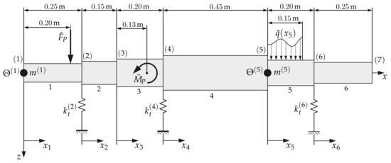
Figure 6. Beam configuration of the numerical example.

The positions $X_i$ of the stations are listed in Table 1, including the lumped masses $m^{\left(i\right)}$, rotary inertia ${\mathsf{\Theta }}^{\left(i\right)}$, and the translational spring constants $k_t^{\left(i\right)}$. Concentrated dampers at the stations are omitted in the numerical example to clearly illustrate the internal damping effect of the material.

Table 1. Coordinates and parameters at the stations.

Station	${\mathit{X}}_{\mathit{i}}$ in $\mathbf{m}$	${\mathit{m}}^{\left(\mathit{i}\right)}$ in $\mathbf{kg}$	${\mathsf{\Theta }}^{\left(\mathit{i}\right)}$ in $\mathbf{kg}{\mathbf{m}}^2$	${\mathit{k}}_{\mathit{t}}^{\left(\mathit{i}\right)}$ in $\frac{\mathbf{N}}{\mathbf{m}}$
1	0.00	2.5	0.6	-
2	0.25	-	-	$3\times {10}^6$
3	0.40	-	-	-
4	0.60	-	-	$8\times {10}^6$
5	1.05	1.5	1.5	-
6	1.25	-	-	$7\times {10}^6$
7	1.50	-	-	-

Each segment ℓ of the beam has a constant circular cross-section, with the diameters $d_1=0.08\mathrm{m}$, $d_2=0.1\mathrm{m}$, $d_3=0.12\mathrm{m}$, $d_4=0.15\mathrm{m}$, $d_5=0.11\mathrm{m}$, and $d_6=0.09\mathrm{m}$. The material of the beam is uniform, and a polymer with high internal damping is chosen to show the dissipative behavior. In Weiß et al. [47], material parameters for PVC are presented, where the fractional Zener model is used to describe the viscoelastic material characteristics. The viscoelastic parameters, adapted to the notation in this paper, are $a_0^E=3.51\times {10}^9\frac{\mathrm{N}}{{\mathrm{m}}^2}$, $a_1^E=8.5486\times {10}^6\frac{{\mathrm{Ns}}^{\alpha }}{{\mathrm{m}}^2}$, $b_0^E=0.002106{\mathrm{s}}^{\alpha }$, and ${\alpha }^E=0.6597$[47]. The material is isotropic with the Poisson’s ratio $\nu =0.38$, and the density of the beam is $\rho =1450\frac{\mathrm{kg}}{{\mathrm{m}}^3}$, which leads to a total beam mass of $23.4\mathrm{kg}$.

The beam is excited by a harmonic concentrated force with the amplitude ${\tilde{F}}_P=20\mathrm{N}$ at $x=0.2\mathrm{m}$ and a point moment with the amplitude ${\tilde{M}}_P=7\mathrm{Nm}$ at $x=0.53\mathrm{m}$. Additionally, a distributed force acts in the fifth segment ($X_{aq}=0\mathrm{m}$ and $X_{bq}=0.15\mathrm{m}$) given by the function $\tilde{q}\left(x_5\right)=200+50·sin\left(64(1.05+x_5)\right)·{(1.05+x_5)}^6\frac{\mathrm{N}}{\mathrm{m}}$, resulting in a total force of $29.9\mathrm{N}$.

The B22 element, which is a planer 3-node quadratic beam element having the Timoshenko theory implemented, is used to build the FEM models. To show the accuracy of the proposed computational technique, a FEM model with a very small element size of $0.001\mathrm{m}$ (6002 degrees of freedom) is applied, which guarantees a highly accurate reference solution. Furthermore, a coarse FEM model (70 degrees of freedom) with a similar computational time as NAT is used to illustrate the computational efficiency of the method. Since the commercial software package Abaqus FEA^® 2017 only supports a complex Young’s modulus, the shear modulus is kept real-valued for the comparison with $G=\frac{a_0^E}{2(1+\nu )}$. For a detailed description of the finite element modeling process, the reader is referred to, e.g., Reference [48].

The frequency response with 2000 frequency steps in the interval of $0\mathrm{Hz}$ to $2000\mathrm{Hz}$ (10 modes) for the response point at $x=0.225\mathrm{m}$ is shown in Figure 7.

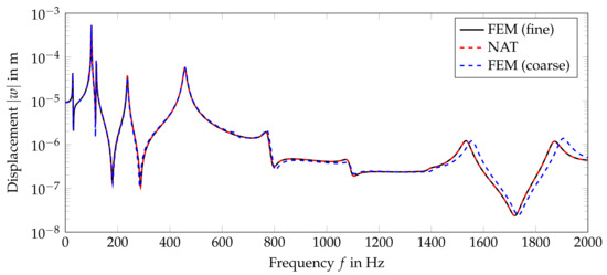
Figure 7. Comparison of the FEM and NAT solutions at $x=0.225\mathrm{m}$ over a wide frequency range.

From Figure 7, it is apparent that NAT gives highly accurate results, since the solutions of the reference model and NAT are not distinguishable. If no distributed loadings are present, NAT even leads to the analytical solution of the problem, due to the analytical homogeneous and particular solutions. The boundary and interface conditions are fulfilled with double-precision. For distributed loadings, a small error occurs when the actual loading is approximated by the Fourier extension method. In the given example, $n=32$ terms are used in the approximation of $\tilde{q}\left(x_5\right)$, which leads to an excellent agreement.

The coarse FEM model, which has a similar order of computational time as NAT, already suffers from certain approximation errors in the higher frequency range, as illustrated in Figure 7. This clearly shows the computational efficiency of NAT compared to element-based techniques. The total computational time of NAT for 2000 frequency points is $7.95\mathrm{s}$, where $6.13\mathrm{s}$ are used to calculate the displacement, rotation, bending moment, and shear force at 1500 locations along the x-axis. Most of the computational time is, therefore, spend on the post-processing step, which can be reduced by a reduction of the evaluation points. Another advantage of NAT compared to FEM is the accuracy of derived quantities, such as the bending moment or shear force, since, in FEM, these quantities are approximated with a lower order polynomial.

In Figure 8, a comparison of the frequency-dependent loss factor $\eta$ and storage modulus $\mathrm{Re}\left[E^{★}\right]$ of the classical Zener model (standard linear solid) and the fractional Zener model is shown. The material parameters of Weiß et al. [47] are used, which are the result from a best fit to measurement data of a PVC beam and plate.

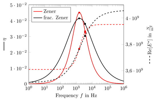
Figure 8. Comparison of the complex modulus for the Zener and fractional Zener model.

While both models show a qualitatively similar behavior having one peak in the loss factor and a monotonically increasing storage modulus, the additional flexibility of the fractional model allows for a better control of the slope in the loss factor curve [11]. Therefore, the actual properties of the viscoelastic material (PVC) are captured more accurately. In Figure 9, the difference of both material models is also clearly visible in the frequency response for the beam system presented in Figure 6.

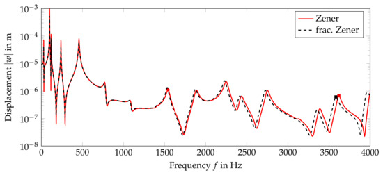
Figure 9. Comparison of the frequency response at $x=0.225\mathrm{m}$ for the classical and fractional Zener model.

The difference in the storage modulus leads to a shifting of the eigenfrequencies between the models, while the different loss factors result in lower or higher amplitudes. The ninth mode at ≈$1540\mathrm{Hz}$ and sixteenth mode at ≈$3600\mathrm{Hz}$ are indicated by bullets and squares in Figure 8 and Figure 9. Since the storage modulus and the loss factor of the classical Zener model are higher at the ninth mode, the eigenfrequency is slightly shifted to the right and the amplitude is reduced compared to the fractional model. At the sixteenth mode, the storage modulus of the classical model is higher, while the loss factor is lower compared to the fractional model. Therefore, the eigenfrequency and the amplitude are greater for the classical material model.

4.2. Comparison with Measurement Data

In this section, the presented numerical method and material model is compared to vibration measurements. Two different cases are considered. In the first case, a beam with a low material damping made of steel is investigated, while the second case shows a beam with high material damping (PVC).

The general test setup of the measurements is equal for both cases. An electrodynamic shaker (type: LDS V406, frequency range: $5\mathrm{Hz}$ to $9\mathrm{kHz}$, maximum force: $196\mathrm{N}$) is used to excite the system, and a force sensor (Brüel & Kjær Type 8230-001, maximum force: $220\mathrm{N}$, linearity error at full scale: ≤$\pm 1\%$) measures the excitation force. A triaxial acceleration sensor (Brüel & Kjær Triaxial Type 4506, frequency range: $0.6\mathrm{Hz}$ to $3000\mathrm{Hz}$) captures the response of the beam. The system is excited with a sinusoidal force at constant frequency, and the response is measured at steady-state conditions. The frequency step is $1\mathrm{Hz}$, and both time signals are transformed into the frequency domain. The ratio of the beam displacement and force amplitude at the excitation frequency is calculated to get the Frequency Response Function (FRF) of the system.

In Figure 10a,b, the test setups of the steel and PVC beam are shown. The multiple-stepped beam $\begin{array}{|c|}\hline a\\ \hline\end{array}$ lies horizontally during the test, and fishing lines $\begin{array}{|c|}\hline d\\ \hline\end{array}$ are used to hold the beam in position. The force sensor including the shaker and stinger $\begin{array}{|c|}\hline b\\ \hline\end{array}$ and the acceleration sensor $\begin{array}{|c|}\hline c\\ \hline\end{array}$ are located in the same horizontal plane. Both sensors are mounted to the surface of the beam using a thin layer of wax. The fishing lines are used to get free boundary conditions at the ends of the beam.

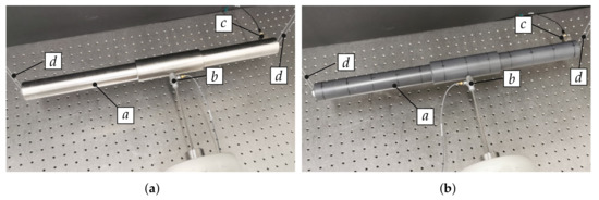
Figure 10. Test setup for the vibration measurements of the beams. (Created by authors.) (a) Steel beam. (b) PVC beam.

The NAT model used to compute the response of the test setup is illustrated in Figure 11. The beam has two steps along the x-axis with the diameters $d_1=d_4=d_5=0.04\mathrm{m}$ and $d_2=d_3=0.05\mathrm{m}$.

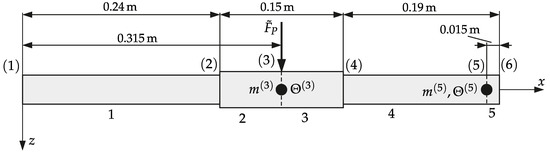
Figure 11. NAT model of the test setup.

The station parameters and locations are listed in Table 2. The excitation due to the electrodynamic shaker is modeled by a simple point force at station (3), since the introduction of a constant distributed force over the force sensor region has a negligible effect on the system response. The response point of the system is located at station $\left(5\right)$. The masses of the sensors are included as lumped masses at the corresponding stations.

Table 2. Station parameters of the beam systems.

Station	${\mathit{X}}_{\mathit{i}}$ in $\mathbf{m}$	${\mathit{m}}^{\left(\mathit{i}\right)}$ in $\mathbf{kg}$	${\mathsf{\Theta }}^{\left(\mathit{i}\right)}$ in $\mathbf{kg}{\mathbf{m}}^2$
1	0.000	-	-
2	0.240	-	-
3	0.315	$0.013$	$8.125\times {10}^{-6}$
4	0.390	-	-
5	0.565	$0.015$	$6.000\times {10}^{-6}$
6	0.580	-	-

4.2.1. Case 1: Steel Beam (Low Damping)

The viscoelastic material parameters of the fractional Zener model are defined by $a_0^E=1.926\times {10}^{11}\frac{\mathrm{N}}{{\mathrm{m}}^2}$, $a_1^E=6.887\times {10}^9\frac{{\mathrm{Ns}}^{\alpha }}{{\mathrm{m}}^2}$, $b_0^E=0.035{\mathrm{s}}^{\alpha }$, and ${\alpha }^E=0.3$, which have been found through a simple optimization approach in MATLAB^®$R2020\mathrm{b}$. The stated parameters are rather different compared to the values presented in Reference [35], which results from the low and nearly frequency independent damping of the material and the limited frequency range. Several parameter combinations lead to a very similar response in the viewed frequency range. Measurements up to a higher frequency would be required to resolve this issue, which is not feasible with the presented test setup. The material is isotropic with $\nu =0.30$, and the density is given by $\rho =7855\frac{\mathrm{kg}}{{\mathrm{m}}^3}$. The shear correction factor is set to $k_S=0.8507$, which is computed with the formulas for circular cross-sections shown in Reference [49].

In Figure 12, a comparison of the measured and calculated FRF is illustrated. There is a general good agreement of both results over the complete frequency range. At higher eigenfrequencies, the measurements are less reliable, since the limits of the applied measurement equipment is reach. Overall, the fractional Zener model is capable of representing the low, nearly frequency independent damping of steel without the drawbacks of the hysteric damping model.

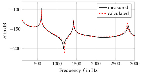
Figure 12. Comparison of the calculated and measured FRFs for the steel beam.

4.2.2. Case 2: PVC Beam (High Damping)

The parameters of the fractional Zener model used to describe the viscoelastic behavior of the PVC are given by $a_0^E=3.272\times {10}^9\frac{\mathrm{N}}{{\mathrm{m}}^2}$, $a_1^E=8.565\times {10}^6\frac{{\mathrm{Ns}}^{\alpha }}{{\mathrm{m}}^2}$, $b_0^E=0.00219{\mathrm{s}}^{\alpha }$, and ${\alpha }^E=0.649$, which are similar to the parameters presented in Reference [47]. The density of the material is given by $\rho =1377\frac{\mathrm{kg}}{{\mathrm{m}}^3}$, and an isotropic behavior with $\nu =0.38$ is assumed. The shear correction factor is calculated as in the previous case, which results in $k_S=0.848$.

A comparison of the measured and calculated FRF is illustrated in Figure 13. The results are in a good agreement over the complete frequency range up to $1000\mathrm{Hz}$. The three eigenfrequencies at around $180\mathrm{Hz}$, $430\mathrm{Hz}$, and $870\mathrm{Hz}$, as well as the amplitudes, are predicted very accurately by the NAT model. It is apparent that the internal damping of the PVC beam is considerable higher compared to the steel beam, since the peaks at the eigenfrequencies are less pronounced. The fractional Zener model is, therefore, also able to describe materials with high internal damping.

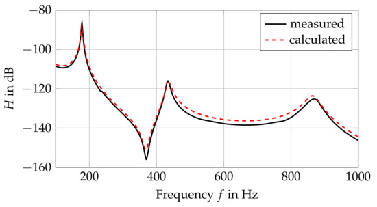
Figure 13. Comparison of the calculated and measured FRFs for the PVC beam.

5. Conclusions

In this paper, a highly accurate and efficient numerical method for the dynamic analysis of viscoelastic beam systems, called Numerical Assembly Technique, has been presented. The viscoelastic behavior of the beam material is described by the fractional Zener model, which allows for the characterization of a wide class of materials with a low number of parameters. Analytical homogeneous solutions of the resulting governing equations have been presented, and analytical solutions for point force and moment excitation have been derived. Semi-analytical solutions for arbitrarily distributed loads have been calculated by an approximation with the Fourier extension method. A comparison to the Finite Element Method has shown the accuracy and efficiency of the proposed numerical method. Vibration measurements for a material with low damping (steel) and high damping (PVC) have been used to validate the material model, showing an overall good agreement between the calculated and measured results.

References

- Han, S.M.; Benaroya, H.; Wei, T. Dynamics of Transversely Vibrating Beams Using Four Engineering Theories. J. Sound Vib. 1999, 225, 935–988. [Google Scholar] [CrossRef]
- Pirrotta, A.; Cutrona, S.; Di Lorenzo, S. Fractional visco-elastic Timoshenko beam from elastic Euler-Bernoulli beam. Acta Mech. 2015, 226, 179–189. [Google Scholar] [CrossRef]
- Rogers, L. Operators and Fractional Derivatives for Viscoelastic Constitutive Equations. J. Rheol. 1983, 27, 351–372. [Google Scholar] [CrossRef]
- Voigt, W. Ueber innere Reibung fester Körper, insbesondere der Metalle. Ann. Phys. 1892, 283, 671–693. [Google Scholar] [CrossRef]
- Maxwell, J.C. On the dynamical theory of gases. Philos. Trans. R. Soc. Lond. 1867, 157, 49–88. [Google Scholar]
- Zener, C.M. Elasticity and Anelasticity of Metals; University of Chicago Press: Chicago, IL, USA, 1948. [Google Scholar]
- Bonfanti, A.; Kaplan, J.L.; Charras, G.; Kabla, A. Fractional viscoelastic models for power-law materials. Soft Matter 2020, 26, 6002–6020. [Google Scholar] [CrossRef]
- Rouleau, L.; Pirk, R.; Pluymers, B.; Desmet, W. Characterization and Modeling of the Viscoelastic Behavior of a Self-Adhesive Rubber Using Dynamic Mechanical Analysis Tests. J. Aerosp. Technol. Manag. 2015, 7, 200–208. [Google Scholar] [CrossRef]
- Pierro, E.; Carbone, G. A new technique for the characterization of viscoelastic materials: Theory, experiments and comparison with DMA. J. Sound Vib. 2021, 515, 116462. [Google Scholar] [CrossRef]
- Failla, G.; Zingales, M. Advanced materials modelling via fractional calculus: Challenges and perspectives. Philos. Trans. R. Soc. Math. Phys. Eng. Sci. 2020, 378, 20200050. [Google Scholar]
- Pritz, T. Analysis of four-parameter fractional derivative model of real solid materials. J. Sound Vib. 1996, 195, 103–115. [Google Scholar] [CrossRef]
- Xu, J.; Chen, Y.; Tai, Y.; Xu, X.; Shi, G.; Chen, N. Vibration analysis of complex fractional viscoelastic beam structures by the wave method. Int. J. Mech. Sci. 2020, 167, 105204. [Google Scholar] [CrossRef]
- Zheng-you, Z.; Gen-guo, L.; Chang-jun, C. Quasi-static and dynamical analysis for viscoelastic Timoshenko beam with fractional derivative constitutive relation. Appl. Math. Mech. 2002, 23, 1–12. [Google Scholar] [CrossRef]
- Pirrotta, A.; Cutrona, S.; Di Lorenzo, S.; Di Matteo, A. Fractional visco-elastic Timoshenko beam deflection via single equation. Int. J. Numer. Methods Eng. 2015, 104, 869–886. [Google Scholar] [CrossRef]
- Usuki, T.; Suzuki, T. Dispersion curves for a viscoelastic Timoshenko beam with fractional derivatives. J. Sound Vib. 2012, 331, 605–621. [Google Scholar] [CrossRef]
- Rossikhin, Y.A.; Shitikova, M.V. Application of Fractional Calculus for Dynamic Problems of Solid Mechanics: Novel Trends and Recent Results. Appl. Mech. Rev. 2010, 63, 010801. [Google Scholar] [CrossRef]
- Loghman, E.; Bakhtiari-Nejad, F.; Kamali, E.A.; Abbaszadeh, M.; Amabili, M. Nonlinear vibration of fractional viscoelastic micro-beams. Int. J. Non-Linear Mech. 2021, 137, 103811. [Google Scholar] [CrossRef]
- Faraji Oskouie, M.; Ansari, R.; Sadeghi, F. Nonlinear vibration analysis of fractional viscoelastic Euler-Bernoulli nanobeams based on the surface stress theory. Acta Mech. Solida Sin. 2017, 30, 416–424. [Google Scholar] [CrossRef]
- Suzuki, J.L.; Kharazmi, E.; Varghaei, P.; Naghibolhosseini, M.; Zayernouri, M. Anomalous Nonlinear Dynamics Behavior of Fractional Viscoelastic Beams. J. Comput. Nonlinear Dyn. 2021, 16, 111005. [Google Scholar] [CrossRef]
- Paunović, S.; Cajić, M.; Karličić, D.; Mijalković, M. A novel approach for vibration analysis of fractional viscoelastic beams with attached masses and base excitation. J. Sound Vib. 2019, 463, 114955. [Google Scholar] [CrossRef]
- Di Paola, M.; Scimemi, F.G. Finite element method on fractional visco-elastic frames. Comput. Struct. 2016, 164, 15–22. [Google Scholar] [CrossRef]
- Wu, J.S.; Chou, H.M. A new approach for determining the natural frequencies and mode shapes of a uniform beam carrying any number of sprung masses. J. Sound Vib. 1999, 220, 451–468. [Google Scholar] [CrossRef]
- Chen, D.W. An exact solution for free torsional vibration of a uniformcircular shaft carrying multiple concentrated elements. J. Sound Vib. 2006, 291, 627–643. [Google Scholar] [CrossRef]
- Yesilce, Y.; Demirdag, O. Effect of axial force on free vibration of Timoshenko multi-span beam carrying multiple spring-mass systems. Int. J. Mech. Sci. 2008, 50, 995–1003. [Google Scholar] [CrossRef]
- Wu, J.S.; Chen, J.H. An efficient approach for determining forced vibration response amplitudes of a MDOF system with various attachments. Shock Vib. 2012, 19, 57–79. [Google Scholar] [CrossRef]
- Yesilce, Y. Free and forced vibrations of an axially-loaded Timoshenko multi-span beam carrying a number of various concentrated elements. Shock Vib. 2012, 19, 735–752. [Google Scholar] [CrossRef][Green Version]
- Klanner, M.; Ellermann, K. Steady-state linear harmonic vibrations of multiple-stepped Euler-Bernoulli beams under arbitrarily distributed loads carrying any number of concentrated elements. Appl. Comput. Mech. 2020, 14, 31–50. [Google Scholar] [CrossRef]
- Wu, J.S.; Lin, F.T.; Shaw, H.J. Analytical Solution for Whirling Speeds and Mode Shapes of a Distributed-Mass Shaft with Arbitrary Rigid Disks. J. Appl. Mech. 2014, 220, 451–468. [Google Scholar] [CrossRef]
- Klanner, M.; Prem, M.S.; Ellermann, K. Steady-state harmonic vibrations of a linear rotor-bearing system with a discontinuous shaft and arbitrary distributed mass unbalance. Proceedings of ISMA2020 International Conference on Noise and Vibration Engineering and USD2020 International Conference on Uncertainty in Structural Dynamics, Leuven, Belgium, 7–9 September 2020; pp. 1257–1272. [Google Scholar]
- Klanner, M.; Prem, M.S.; Ellermann, K. Quasi-analytical solutions for the whirling motion of multi-stepped rotors with arbitrarily distributed mass unbalance running in anisotropic linear bearings. Bull. Pol. Acad. Sci. Tech. Sci. 2021, 69, e138999. [Google Scholar]
- Wu, J.S.; Chen, C.T. A continuous-mass TMM for free vibration analysis of a non-uniform beam with various boundary conditions and carrying multiple concentrated elements. J. Sound Vib. 2008, 311, 1420–1430. [Google Scholar] [CrossRef]
- Banerjee, J.R. Review of the dynamic stiffness method for free-vibration analysis of beams. Transp. Saf. Environ. 2019, 1, 106–116. [Google Scholar] [CrossRef]
- Huybrechs, D. On the Fourier Extension of Nonperiodic Functions. SIAM J. Numer. Anal. 2010, 47, 4326–4355. [Google Scholar] [CrossRef]
- Bauchau, O.A.; Craig, J.I. Structural Analysis—With Applications to Aerospace Structures; Springer: Dordrecht, The Netherlands, 2009. [Google Scholar]
- Caputo, M.; Mainardi, F. Linear Models of Dissipation in Anelastic Solids. Riv. Nuovo C. 1971, 1, 161–198. [Google Scholar] [CrossRef]
- Gaul, L.; Klein, P.; Kemple, S. Damping description involving fractional operators. Mech. Syst. Signal Process. 1991, 5, 81–88. [Google Scholar] [CrossRef]
- Bagley, R.L.; Torvik, P.J. A Theoretical Basis for the Application of Fractional Calculus to Viscoelasticity. J. Rheol. 1983, 27, 201–210. [Google Scholar] [CrossRef]
- Hagedorn, P.; DasGupta, A. Vibrations and Waves in Continuous Mechanical Systems; John Wiley & Sons: Chichester, UK, 2007. [Google Scholar]
- Rao, S.S. Vibration of Continuous Systems; John Wiley & Sons: Hoboken, NJ, USA, 2019. [Google Scholar]
- Debnath, L.; Bhatta, D. Integral Transforms and Their Applications; CRC Press: Boca Raton, FL, USA, 2015. [Google Scholar]
- Mitrinović, D.; Kečkić, J.D. The Cauchy Method of Residues; D. Reidel Publishing Company: Dordrecht, The Netherlands, 1984. [Google Scholar]
- Hayek, S.I. Advanced Mathematical Methods in Science and Engineering; CRC Press: Boca Raton, FL, USA, 2010. [Google Scholar]
- Adcock, B.; Huybrechs, D.; Martín-Vaquero, J. On the Numerical Stability of Fourier Extensions. Found. Comput. Math. 2014, 14, 638–687. [Google Scholar] [CrossRef][Green Version]
- Matthysen, R.; Huybrechs, D. Fast Algorithms for the Computation of Fourier Extensions of Arbitrary Length. SIAM J. Sci. Comput. 2016, 38, A899–A922. [Google Scholar] [CrossRef]
- Lyon, M. A Fast Algorithm for Fourier Continuation. SIAM J. Sci. Comput. 2011, 33, 3241–3260. [Google Scholar] [CrossRef]
- Adcock, B.; Huybrechs, D. On the resolution power of Fourier extensions for oscillatory functions. J. Comput. Appl. Math. 2014, 260, 312–336. [Google Scholar] [CrossRef][Green Version]
- Weiß, M.; Lerch, R.; Rupitsch, S.J. Simulation-Based Material Characterization of Isotropic and Direction-Dependent Polymers for Use in Active Structure Assemblies. Adv. Eng. Mater. 2018, 20, 1800417. [Google Scholar] [CrossRef]
- Bathe, K.J. Finite Element Procedures; Prentice Hall: Hoboken, NJ, USA, 2006. [Google Scholar]
- Steinboeck, A.; Kugi, A.; Mang, H.A. Energy-consistent shear coefficients for beams with circular cross sectionsand radially inhomogeneous materials. Int. J. Solids Struct. 2013, 50, 1859–1868. [Google Scholar] [CrossRef]
Publisher’s Note: MDPI stays neutral with regard to jurisdictional claims in published maps and institutional affiliations. |
© 2021 by the authors. Licensee MDPI, Basel, Switzerland. This article is an open access article distributed under the terms and conditions of the Creative Commons Attribution (CC BY) license (https://creativecommons.org/licenses/by/4.0/).