A Biologically Motivated, Proto-Object-Based Audiovisual Saliency Model

Abstract

The natural environment and our interaction with it are essentially multisensory, where we may deploy visual, tactile and/or auditory senses to perceive, learn and interact with our environment. Our objective in this study is to develop a scene analysis algorithm using multisensory information, specifically vision and audio. We develop a proto-object-based audiovisual saliency map (AVSM) for the analysis of dynamic natural scenes. A specialized audiovisual camera with 360${}^{\circ }$ field of view, capable of locating sound direction, is used to collect spatiotemporally aligned audiovisual data. We demonstrate that the performance of a proto-object-based audiovisual saliency map in detecting and localizing salient objects/events is in agreement with human judgment. In addition, the proto-object-based AVSM that we compute as a linear combination of visual and auditory feature conspicuity maps captures a higher number of valid salient events compared to unisensory saliency maps. Such an algorithm can be useful in surveillance, robotic navigation, video compression and related applications.

1. Introduction

Scientists and engineers have traditionally separated the analysis of a multisensory scene into its constituent sensory domains. In this approach, for example, all auditory events are processed separately and independently of visual and/or somatosensory streams, even though the same multisensory event might have created those constituent streams. It was previously necessary to compartmentalize the analysis because of the sheer enormity of information as well as the limitations of experimental techniques and computational resources. With recent advances, it is now possible to perform integrated analysis of sensory systems including interactions within and across sensory modalities. Such efforts are becoming increasingly common in cellular neurophysiology, imaging and psychophysics studies [1,2,3,4,5].

Recent evidence from neuroscience [1,6] suggests that the traditional view that the low level areas of cortex are strictly unisensory, processing sensory information independently, which is later on merged in higher level associative areas is increasingly becoming obsolete. This has been proved by many fMRI [7,8], EEG [9] and neuro-physiological experiments [10,11] at various neural population scales. There is now enough evidence to suggest an interplay of connections among thalamus, primary sensory and higher level association areas which are responsible for audiovisual integration. The broader implications of these biological findings may be that learning, memory and intelligence are tightly associated with the multi-sensory nature of the world.

Hence, incorporating this knowledge in computational algorithms can lead to better scene understanding and object recognition for which there is a great need. Moreover, combining visual and auditory information to associate visual objects with their sounds can lead to better understanding of events. For example, discerning whether the bat hit the baseball during a swing of the bat, tracking objects under severe occlusions or poor lighting conditions, etc. can be more accurately performed only when we take audio and visual counterparts together. The applications of such technologies are numerous and in varied fields.

Kimchi et al. [12] showed that objects attract human attention in a bottom-up manner. In addition, Nuthmann and Henderson [13] found that eye fixations of human observers tend to coincide with object centers. Simple pixel based saliency models determine salient locations based on dissimilarities in low-level features such as color, orientation, etc, which do not always coincide with object centers. In a proto-object-based saliency model, the grouping mechanism integrates border ownership (Section 3.3) information in an annular fashion to create selectivity for objects. This is based on Gestalt properties of convexity, surroundedness and parallelism. Hence, the predicted salient locations in our model generally coincide with object centers, which cannot be achieved with simple feature-based saliency models.

Even though processing of sensory information in the brain involves a combination of feed-forward, feedback and recurrent connections in the neural circuitry, the advantage of a feed-forward model is that information is processed in a single pass, hence making it fast and suitable for real-world applications. Motivated by these factors, we develop a purely bottom-up, proto-object-based audiovisual saliency map (AVSM) for the analysis of dynamic natural scenes.

For the computation of AVSM, we need both audio and video data in the same co-ordinate system. Thus, as shown in Figure 1, we stitch together images from different views to get a 360${}^{\circ }$ panoramic view of the scene. Similarly, direction and loudness of sound sources in the scene are estimated from multi-channel audio sampled on the surface of a sphere. Both video and audio are registered such that they are in the same reference frame. Such spatiotemporally registered audiovisual data are used for saliency map computation, as described in Section 3. We add visual motion (Section 3.1.1) as another independent feature type along with color, intensity and orientation [14], all of which undergo a grouping process (Section 3.4) to form proto-objects of each feature type. In the auditory domain, we consider the location and intensity of sound as the only proto-objects as these are found to be most influential in drawing the spatial attention of an observer in many psycho-physics studies. Various methods of combination of the auditory and visual proto-object features are considered (Section 3.6). We demonstrate the efficacy of the AVSM in predicting salient locations in the audiovisual environments by testing it on real world AV data collected from specialized hardware (Section 4) that can collect 360${}^{\circ }$ audio and video that are temporally synchronized and spatially co-registered. The AVSM captures nearly all visual, auditory and audio-visually salient events, just as any human observer would notice in that environment.

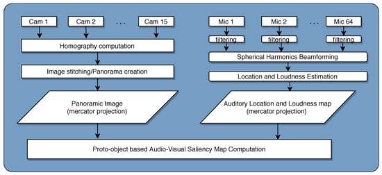
Figure 1. Overall architecture of the model: Video frames from 15 HD RGB cameras are stitched together to form a 360${}^{\circ }$ panoramic view of the scene. Audio from 64 microphones are filtered and spherical harmonic beamforming (see Section 4 for details) is done to estimate the direction and loudness of different auditory sources in the scene. Both video stitching and audio beamforming are initially done on the surface of a unit sphere, later projected to 2D plane using mercator projection. The audio and video are in perfect spatiotemporal register, so there is a one-to-one correspondence between the visual object and auditory sound source in the scene. The 2D maps are then used to compute the Audio Visual Saliency Map as described in Figure 2.

In summary, a better understanding of interaction, information integration and complementarity of information across senses may help us build many intelligent algorithms for scene analysis, object detection and recognition, human activity and gait detection, elder/child care and monitoring, surveillance, robotic navigation, biometrics, etc. with better performance, stability and robustness to noise. In one application, for example, fusing auditory (voice) and visual (face) features improved the performance of speaker identification and face recognition systems [15,16]. Hence, our objective in this study is to develop a scene analysis algorithm using multisensory information, specifically vision and audio.

2. Related Work

The study of multi-sensory integration [3,6,17], specifically audiovisual integration [4,18], has been an active area of research in neuroscience, psychology and cognitive science. In the computer science and engineering fields, there is an increased interest in the recent times [19,20,21]. For a detailed review of neuroscience and psychophysics research related to audiovisual interaction, please refer to [3,17]. Here, we restrict our review to models of perception in audiovisual environments and some application oriented research using audio and video information.

In one of the earliest works [22], a one-dimensional computational neural model of saccadic eye movement control by Superior Colliculus (SC) is investigated. The model can generate three different types of saccades: visual, multimodal and planned. It takes into account different coordinate transformations between retinotopic and head-centered coordinate systems, and the model is able to elicit multimodal enhancement and depression that is typically observed in SC neurons [23,24]. However, the main focus is on Superior Colliculus function rather than studying audiovisual interaction from a salience perspective. A detailed model of the SC is presented in [25] with the aim of localizing audiovisual stimuli in real time. The model consists of 12,240 topographically organized neurons, which are hierarchically arranged into nine feature maps. The receptive field of these neurons, which are fully connected to their input, are obtained through competitive learning. Intra-aural level differences are used to model auditory localization, while simple spatial and temporal differencing is used to model visual activity. A spiking neuron model [26] of audiovisual integration in barn owl uses Spike Timing Dependent Plasticity (STDP) to modulate activity dependent axon development, which is responsible for aligning visual and auditory localization maps. A neuromorphic implementation of the same using digital and analog mixed Very Large Scale Integration (mixed VLSI) can be found in [27].

In another neural model [28,29], the visual and auditory neural inputs to the deep SC neuron are modeled as Poisson random variables. Their hypothesis is that the response of SC neurons is proportional to the presence of an audiovisual object/event in that spatial location which is conveyed to topographically arranged deep SC neurons via auditory and visual modalities. The model is able to elicit all properties of the SC neurons. An information theoretic explanation of super-additivity and other phenomena is given in a [29]. The authors also showed that addition of a cue from another sensory modality increases the certainty of a target’s location only if the input from initial modality/modalities cannot reduce the uncertainty about target. Similar models are proposed in [30,31], where the problem is formulated based on Bayes likelihood ratio. An important work [32] based on Bayesian inference explains a variety of cue combination phenomena including audiovisual spatial location estimation. According to the model, neuronal populations encode stimulus information using probabilistic population codes (PPCs) which represent probability distributions of stimulus properties of any arbitrary distribution and shape. The authors argued that neural populations approximate the Bayes rule using simple linear combination of neuronal population activities.

In [33], audiovisual arrays for untethered spoken interfaces are developed. The arrays localize the direction and distance of an auditory source from the microphone array, visually localize the auditory source, and then direct the microphone beamformer to track the speaker audio-visually. The method is robust to varying illumination and reverberation, and the authors reported increased speech recognition accuracy using the AV array compared to non-array based processing.

In [34], the authors found that emotional saliency conveyed through audio, drags an observer’s attention to the corresponding visual object, hence people often fail to notice any visual artifacts present in the video, suggest to exploit this property in intelligent video compression. For the same goal, the authors of [35] implemented an efficient video coding algorithm based on the audiovisual focus of attention where sound source is identified from the correlation between audio and visual motion information. The same premise that audiovisual events draw an observer’s attention is the basis for their formulation. A similar approach is applied to high definition video compression in [36]. In these studies, spatial direction of sound was not considered; instead, stereo or mono audio track accompanying the video was used in all computational and experimental work.

In [37], a multimodal bottom-up attentional system consisting of a combined audiovisual salience map and selective attention mechanism is implemented for the humanoid robot iCub. The visual salience map is computed from color, intensity, orientation and motion maps. The auditory salience map consists of the location of the sound source. Both are registered in ego-centric coordinates. The audiovisual salience map is constructed by performing a pointwise $\max \left(\right)$ operation on visual and auditory maps. In an extension to multi-camera setting [38], the 2D saliency maps are projected into a 3D space using ray tracing and combined as a fuzzy aggregations of salience spaces. In [39,40], after computing the audio and visual saliency maps, each salient event/proto-object is parameterized by salience value, cluster center (mean location) and covariance matrix (uncertainty in estimating location). The maps are linearly combined based on [41]. Extensions of this approach can be found in [42]. A work related to the one in [42] is presented in [43], where a weighted linear combination of proto-object representations obtained using mean-shift clustering is detailed. Even though the method uses linear combination, the authors did not use motion information in computing the visual saliency map. A Self Organizing Map (SOM)-based model of audiovisual integration is presented in [44], in which the transformations between sensory modalities and the respective sensory reliabilities are learned in an unsupervised manner. A system to detect and track a speaker using a multi-modal, audiovisual sensor set that fuses visual and auditory evidence about the presence of a speaker using Bayes network is presented in [45]. In a series of papers [19,46,47], audiovisual saliency is computed as a linear mixture of visual and auditory saliency maps for the purpose of movie summarization and key frame detection. No spatial information about audio is considered. The algorithm performs well in summarizing the videos for informativeness and enjoyability for movie clips of various genres. An extension of these models incorporating text saliency can be found in [48]. By assuming a single moving sound source in the scene, audio was incorporated into the visual saliency map in [49], where sound location was associated with the visual object by correlating sound properties with the motion signal. By computing Bayesian surprise as in [50], the authors of [51] presented a visual attention model driven by auditory cues, where surprising auditory events are used to select synchronized visual features and emphasize them in an audiovisual surprise map. A real-time multi-modal home entertainment system [52] performing a just-in-time association of features related to a person from audio and video are fused based on the shortest distance between each of the faces (in video) and the audio direction vector. In an intuitive study [53], speaker localization by measuring the audiovisual synchrony in terms of mutual information between auditory features and pixel intensity change is considered. In a single active speaker scenario, the authors obtained good preliminary results. No microphone arrays are used for the localization task. In [54], visually detected face location is used to improve the speaker localization using a microphone array. A fast audiovisual attention model for human detection and localization is proposed in [55].

The effect of sound on gaze behavior in videos is studied in [20,56], where a preliminary computational model to predict eye movements is proposed. The authors used motion information to detect sound source. High level features such as face are hand labeled. A comparison of eye movements during visual only and audiovisual conditions with their model shows that adding sound information improves the predictive power of their model. The role of salience, faces and sound in directing the attention of human observers (measured by gaze tracking) is studied with psychophysics experiments and computational modeling in [57], and an audiovisual attention model for natural conversation scenes is proposed in [58], where the authors used a speaker diarization algorithm to compute saliency. Even though their study is restricted to conversation of humans and not applicable any generic audiovisual scene, hence cannot be regarded as a generalized model of audiovisual saliency, some interesting results are shown. Using EM algorithm to determine the individual contributions of bottom-up salience, faces and sound in gaze prediction, the authors showed that adding original speech to video improves gaze predictability, whereas adding irrelevant speech or unrelated natural sounds has no effect. By using speaker diarization algorithm [58], when the weight for active speakers is increased, their audiovisual attention model significantly outperforms the visual saliency model with equal weights for all faces. An audiovisual saliency map is developed in [59] where features such as color, intensity, orientation, faces and speech are linearly combined with unequal weights to give different types of saliency maps depending on the presence/absence of faces and/or speech. It is not clear as to whether location of the sound is used in this approach. In addition, the authors did not factor in motion, which is an important feature, while designing a saliency map for moving pictures.

More recently, there have been some efforts related to audiovisual saliency [60,61,62,63], but very few explicitly incorporate spatial (two-dimensional) audio [62]. However, some of the drawbacks of those models are that they are not based on the neural principles and do not use spatial audio which is an important feature in the auditory domain. Even more importantly, traditional saliency models do no have a notion of proto-objects. In our work, saliency is computed based on proto-objects which helps to localize salient object centers, rather than sharp discontinuities.

3. Model Description

The computation of audiovisual saliency map is similar to the computation of proto-object-based visual saliency map for static images explained in [14], except for: (i) the addition of two new feature channels, the visual motion channel and the auditory loudness and location channel; and (ii) different ways of combining the conspicuity maps to get the final saliency maps. Hence, whenever the computation is identical to the one in [14], we only give a gist of that computation to avoid repetition and detailed explanation otherwise.

The AVSM is computed by grouping auditory and visual bottom-up features at various scales, then normalizing the grouped features within and across scales, followed by merging features across scales and linear combination of the resulting feature conspicuity maps (Figure 2). The features are derived from the color video and multi-channel audio input (Section 4) without any top-down attentional biases, hence the computation is purely bottom-up. The mechanism of grouping “binds” features within a channel into candidate objects or “proto-objects”. Approximate size and location are the only properties of objects that the grouping mechanism estimates, hence they are termed “proto-objects”. Many such proto-objects form simultaneously and dissolve rapidly [64] in a purely bottom-up manner. Top-down attention is required to hold them together into coherent objects.

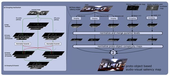
Figure 2. Computation of proto-object-based AVSM. (a) Grouping mechanism: At each scale, feature maps are filtered with center-surround cells, normalized, followed by border ownership (BO) computation. Grouping cells, at each scale, receive a higher feed-forward input from BO cells if they are consistent with Gestalt properties of convexity, proximity and surroundedness. Hence, grouping gathers conspicuous BO activity of features at object centers. Each feature channel undergoes same computation at various scales (except orientation, see explanation); only the intensity channel shown in (a). (b) Audiovisual saliency computation mechanism: Five feature types are considered: color, orientation, intensity and motion in the visual domain and spatial location and loudness estimate in the auditory domain. All features undergo grouping as explained in (a) to obtain proto-object pyramids. The proto-object pyramids are normalized, collapsed to get the feature specific conspicuity maps such that isolated strong activity is accentuated and distributed weak activity is suppressed. The conspicuity maps are then combined in different ways, as explained in Section 3.6, to get different saliency maps. Figure adapted with permission from [14].

In addition, computation of AVSM is completely feed-forward. Many spatial scales are used to achieve scale invariance. First, the independent feature maps are computed; features within each channel are grouped into proto-objects. Such proto-object feature pyramids at various scales are normalized within and across scales. Such feature pyramids are merged across scales followed by normalization across feature channels to give rise to conspicuity maps. The conspicuity maps are linearly combined to get the final AVSM. Each of these steps is explained in more detail below.

3.1. Computation of Feature Channels

We consider color, intensity, orientation and motion as separate, independent feature channels in the visual domain and loudness and spatial location as features in the auditory space. The audiovisual camera equipment used for data gathering (see Section 4) guarantees spatial and temporal concurrency of audio and video.

A single intensity channel, where intensity is computed as the average of red, green and blue color channels, is used. Four feature sub-channels for angle, $\theta =\{0,\frac{\pi }{4},\frac{\pi }{2},\frac{3\pi }{4}\}$ are used for orientation channel. Four color opponency feature sub-channels—red–green ($\mathcal{RG}$), green–red ($\mathcal{GR}$), blue–yellow ($\mathcal{BY}$) and yellow–blue ($\mathcal{YB}$)—are used for color channel. The computation of color, orientation and intensity feature channels is identical to Russell et al. [14].

Visual motion, auditory loudness and location estimate are the newly added features, the computation of which is explained below.

3.1.1. Visual Motion Channel

Motion is computed using the optical flow algorithm described in [65] and the corresponding code available at [66]. Consider two successive video frames, $I(x,y,t)$ and $I(x,y,t+1)$. If the underlying object has moved between t and $t+1$, then the intensity at pixel location $(x,y)$ at time t should be the same as in a nearby pixel location at $(x+\Delta x,y+\Delta y)$ in the successive frame at $t+1$. Using this as one of the constraints, the flow is estimated which gives the horizontal and vertical velocity components, $u(x,y,t)$ and $v(x,y,t)$, respectively, at each pixel location $(x,y)$ at time t. For a more detailed explanation, see [65]. Since we are interested in detecting salient events only, we do not take into account the exact motion at each location as given by $u(x,y,t)$ and $v(x,y,t)$; instead, we look at how big the motion is at each location in the image. The magnitude of motion at each location is computed as,

$$M(x,y,t)=\sqrt{u{(x,y,t)}^2+v{(x,y,t)}^2}$$

(1)

The motion map $M(x,y,t)$ gives the magnitude of motion at each location in the visual scene at different time instances t. Figure 3A,B shows two successive frames of the video. The computed magnitude of motion using the optic flow method in [65] is shown in Figure 3C. The person in the video is the only moving source.

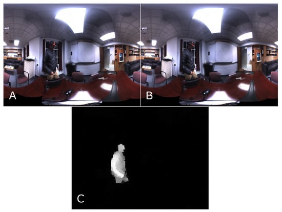
Figure 3. Computation of motion magnitude map: (A) a frame from the dataset; and (B) the successive frame. The person in the two frames is the only moving object in the two image frames, moving from left to right in the image. (C) The motion magnitude map.

3.1.2. Auditory Loudness and Location Channel

The auditory input consists of a recording of the 3D sound field using 64 microphones arranged on a sphere (see Section 4 for details). We compute a single map for both loudness and location of sound sources $A(x,y,t)$. The value at a location in the map $A(x,y,t)$ gives an estimate of loudness at that location at time t; hence, we simultaneously get the presence and loudness of sound sources at every location in the entire environment. These two features are computed using the beamforming technique, as described in [67,68,69]. A more detailed account is given in Section 4. Two different frames of video and the corresponding auditory loudness and location maps superimposed on the visual images are shown in Figure 4B,F respectively. Warm colors indicate higher intensity of sound from that location in the video.

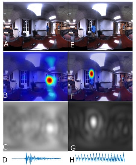
Figure 4. Computation of auditory location and loudness map: two different video frames (A,E); the corresponding audio samples from one of the audio channels, which display only 4410 samples, i.e., audio of 0.1 s (D,H); the corresponding auditory loudness and location maps (C,G); and the corresponding video overlays, which are for illustration only, not used in any computation (B,F). (Left) Sound of a clap; and (Right) some part of the word “eight” uttered by the person.

3.2. Feature Pyramid Decomposition

Feature pyramids are computed for each type. As the scale increases, the resolution of the feature map decreases. The feature maps of successively higher scales are computed by downsampling the feature map from the previous scale. The downsampling factor can be either $\sqrt{2}$ (half-octave) or 2 (full octave). The feature pyramids thus obtained are used to compute proto-objects by border ownership and grouping computation process explained the next two sections.

3.3. Border Ownership Pyramid Computation

Computation of proto-objects by grouping mechanism can be divided into two sub-steps: (i) border ownership pyramid computation; and (ii) grouping pyramid computation.

The operations performed on any of the features, auditory or visual, is the same. Edges of four orientations, $\theta =\{0,\pi /4,\pi /2,3\pi /4\}$ are computed using the Gabor filter bank. The V1 complex cell responses [14] thus obtained are used to construct the edge pyramids. Border ownership response is computed by modulating the edge pyramid by the activity of center-surround feature differences on either side of the border. The rationale behind this was the observation made by Zhang and von der Heydt [70], who reported that the activity border ownership cells was enhanced when image fragments were placed on their preferred side, but suppressed for the non-preferred side.

Two types of center-surround (CS) feature pyramids are used. The center-surround light pyramid detects strong features surrounded by weak ones. Similarly, to detect weak features surrounded by a strong background, a center-surround dark pyramid is used. The rationale behind light and dark CS pyramids is that there can be bright objects on a dark background and vice versa. The center-surround pyramids are constructed by convolving feature maps with Difference of Gaussian (DoG) filters.

The CS pyramid computation is performed in this manner for all feature types including motion and audio, except for the orientation channel. For the orientation feature channel, the DoG filters are replaced by the even symmetric Gabor filters which detect edges. This is because, for the orientation channel, feature contrasts are not typically symmetric as in the case of other channels, but oriented at a specific angle.

An important step in the border ownership computation is normalization of the center-surround feature pyramids. We follow the normalization method used in [71], which enhances isolated high activities and suppresses many closely clustered similar activities.

This normalization step enables comparison of light and dark CS pyramids. Because of the normalization, border ownership activity and grouping activity are proportionately modulated, deciding relative salience of proto-objects from the grouping activity.

The border ownership (BO) pyramids corresponding to light and dark CS pyramids are constructed by modulating the edge activity by the normalized CS pyramid activity. The light and dark BO pyramids are merged across scales and summed to get contrast polarity invariant BO pyramids. For each orientation, two BO pyramids with opposite BO preferences are be computed. From this, the winning BO pyramids are computed by a winner-take-all mechanism.

3.4. Grouping Pyramid Computation

The grouping computation shifts the BO activity from edge pixels to object centers. Grouping pyramids are computed by integrating the winning BO pyramid activity such that selectivity for Gestalt properties of convexity, proximity and surroundedness is enhanced. This is done by using grouping (G) cells in this computation, which have an annular receptive field. The shape of G cells gives rise to selectivity for convex, surrounded objects. At this stage, we have the grouping or proto-object pyramids which are normalized and combined across scales to compute feature conspicuity maps, and then the saliency map.

3.5. Normalization and Across-Scale Combination of Grouping Pyramids

The computation of grouping pyramids as explained in Section 3.4 is performed for each feature type. Let us represent the grouping pyramid for intensity feature channel by ${\mathcal{G}}_{\mathcal{I}}^k(x,y,t)$, where k denotes the scale of the proto-object map in the grouping pyramid. The color feature sub-channel grouping pyramids are represented as ${\mathcal{G}}_{\mathcal{RG}}^k(x,y,t)$ for red–green, ${\mathcal{G}}_{\mathcal{GR}}^k(x,y,t)$ for green–red, ${\mathcal{G}}_{\mathcal{BY}}^k(x,y,t)$ for blue–yellow and ${\mathcal{G}}_{\mathcal{YB}}^k(x,y,t)$ for yellow–blue color opponencies. The orientation grouping pyramids are denoted by ${\mathcal{G}}_{\mathcal{O}}^k(x,y,t,\theta )$ where $\theta$ denotes orientation, motion feature channel by ${\mathcal{G}}_{\mathcal{M}}^k(x,y,t)$ and auditory location and intensity feature channel by ${\mathcal{G}}_{\mathcal{A}}^k(x,y,t)$. The corresponding conspicuity maps for, intensity $\mathcal{I}(x,y,t)$, color $\mathcal{C}(x,y,t)$, orientation $\mathcal{O}(x,y,t)$, motion, $\mathcal{M}(x,y,t)$ and auditory location and loudness estimate, $\mathcal{A}(x,y,t)$ are, respectively, obtained as,

$$\mathcal{I}(x,y,t)=\underset{k=1}{\overset{k=10}{⨁}}\mathcal{N}\left({\mathcal{G}}_{\mathcal{I}}^k(x,y,t)\right)$$

(2)

$$\begin{array}{c}\hfill \mathcal{C}(x,y,t)=\underset{k=1}{\overset{k=10}{⨁}}(\mathcal{N}\left({\mathcal{G}}_{\mathcal{RG}}^k(x,y,t)\right)+\mathcal{N}\left({\mathcal{G}}_{\mathcal{GR}}^k(x,y,t)\right)\\ \hfill +\mathcal{N}\left({\mathcal{G}}_{\mathcal{BY}}^k(x,y,t)\right)+\mathcal{N}\left({\mathcal{G}}_{\mathcal{YB}}^k(x,y,t)\right))\end{array}$$

(3)

$$\mathcal{O}(x,y,t)=\underset{k=1}{\overset{k=10}{⨁}}\sum _{\theta \in \{0,\frac{\pi }{4},\frac{\pi }{2},3\frac{\pi }{4}\}}\mathcal{N}\left({\mathcal{G}}_{\mathcal{O}}^k(x,y,t,\theta )\right)$$

(4)

$${\displaystyle \mathcal{M}(x,y,t)=\underset{k=1}{\overset{k=10}{⨁}}\mathcal{N}\left({\mathcal{G}}_{\mathcal{M}}^k(x,y,t)\right)}$$

(5)

$${\displaystyle \mathcal{A}(x,y,t)=\underset{k=1}{\overset{k=10}{⨁}}\mathcal{N}\left({\mathcal{G}}_{\mathcal{A}}^k(x,y,t)\right)}$$

(6)

where $\mathcal{N}(.)$ is a normalization step as explained by Itti et al. [71], which accentuates strong isolated activity and suppresses many weak activities, the symbol ⨁ denotes “across-scale” addition of the proto-object maps, which is done by resampling (up- or down-sampling depending on the scale, k) maps at each level to a common scale (in this case, the common scale is $k=8$) and then doing pixel-by-pixel addition. We use the same set of parameters as in Table 1 of Russell et al. [14] for our computation as well.

The conspicuity maps, due to varied number of feature sub-channels, have different ranges of activity; hence, if we linearly combine without any rescaling to a common scale, those features with higher number of sub-channels may dominate. Hence, each feature conspicuity map is rescaled to the same range, $[0,\dots ,1]$. The conspicuity maps are combined in different ways to get different types of saliency maps, as explained in Section 3.6.

3.6. Combination of Conspicuity Maps

The visual saliency map is computed as,

$$\begin{array}{c}\hfill \mathcal{VSM}(x,y,t)=w_I\mathcal{R}\left(\mathcal{I}(x,y,t)\right)+w_C\mathcal{R}\left(\mathcal{C}(x,y,t)\right)\\ \hfill +w_O\mathcal{R}\left(\mathcal{O}(x,y,t)\right)+w_M\mathcal{R}\left(\mathcal{M}(x,y,t)\right)\end{array}$$

(7)

where $\mathcal{VSM}(x,y,t)$ is the visual saliency map, $\mathcal{R}(.)$ is the rescaling operator that rescales each map to the same range, $[0,\dots ,1]$, and $w_I,w_C,w_O$ and $w_M$ are the individual weights for intensity, color, orientation and motion conspicuity maps, respectively. In our implementation, all weights are equal and each is set to 0.25, i.e., $w_I=w_C=w_O=w_M=\frac{1}{4}$.

Since audio is a single feature channel, the conspicuity map for auditory location and loudness is also the auditory saliency map, $\mathcal{ASM}(x,y,t)$.

We compute the audiovisual saliency map in three different ways to compare the most effective method to identify salient events (see Section 5 for related discussion).

In the first method, a weighted combination of all feature maps is done to get the audiovisual saliency map as,

$$\begin{array}{c}\hfill {\mathcal{AVSM}}_1(x,y,t)=w_I\mathcal{R}\left(\mathcal{I}(x,y,t)\right)+w_C\mathcal{R}\left(\mathcal{C}(x,y,t)\right)+w_O\mathcal{R}\left(\mathcal{O}(x,y,t)\right)\\ \hfill +w_M\mathcal{R}\left(\mathcal{M}(x,y,t)\right)+w_A\mathcal{R}\left(\mathcal{A}(x,y,t)\right)\end{array}$$

(8)

where different weights can be set for $w_{(.)}$ such that the sum of all weights equals 1. In our implementation, all weights are set equal, i.e., $w_I=w_C=w_O=w_M=w_A=\frac{1}{5}$.

In the second method, the visual saliency map is computed as in Equation (7) and then a simple average of the visual saliency map and the auditory conspicuity map (also auditory saliency map, $\mathcal{ASM}(x,y,t)$) is computed to get the audiovisual saliency map as,

$${\mathcal{AVSM}}_2(x,y,t)=\frac{1}{2}\left(\mathcal{R}\left(\mathcal{VSM}\right(x,y,t\left)\right)+\mathcal{R}\left(\mathcal{A}\right(x,y,t\left)\right)\right)$$

(9)

The distribution of weights in Equation (9) is different from that in Equation (8). In Method 2, a “late combination” of the visual and auditory saliency maps is performed, which results in an increase in the weight of the auditory saliency map and a reduction in weights for the individual feature conspicuity maps of the visual domain.

In the last method, in addition to a linear combination of the visual and auditory saliency maps, a product term is added as,

$$\begin{array}{c}\hfill {\mathcal{AVSM}}_3(x,y,t)=(\mathcal{R}\left(\mathcal{VSM}(x,y,t)\right)+\mathcal{R}\left(\mathcal{A}(x,y,t)\right)\\ \hfill +\mathcal{R}\left(\mathcal{VSM}\right(x,y,t\left)\right)\otimes \mathcal{R}\left(\mathcal{A}\right(x,y,t\left)\right))\end{array}$$

(10)

where the symbol ⊗ denotes a point-by-point multiplication of pixel values of the corresponding saliency maps. The effect of the product term is to increase the saliency of those events that are salient in both visual and auditory domains, thereby to enhance the saliency of spatiotemporally concurrent audiovisual events. A comparison of the different saliency maps in detecting salient events is in Section 5.

4. Data and Methods

Audiovisual data were collected using the VisiSonics RealSpace^TM audiovisual camera [67,69]. The AV camera consists of a spherical microphone array with 64 microphones arranged on a sphere of 8 inches diameter and 15 HD cameras arranged on the same sphere (Figure 5). Each video camera can record color (RGB) videos at a resolution of $1328\times 1044$ pixels per frame and 10 frames per second. The audio channels record high fidelity audio at a sampling rate of 44.1 kHz per channel. The audio and video data were converted into a single USB 3.0 compliant stream which is accepted by a laptop computer with Graphical Processing Units. The individual videos are stitched together to produce a panoramic view of the scene in two different projection types: spherical and Mercator. The audio and video streams were synchronized by an internal Field Programmable Gate Array (FPGA)-based processor. The equipment can be used to localize sounds and display them on the panoramic video in real time and also record AV data for later analysis. The length of each recording can be set at any value between 10 and 390 s. The gain for each recording session can be set to three predefined values: −20, 0 and +20 dB. This is particularly helpful to record sounds with high fidelity in indoor, outdoor and noisy conditions.

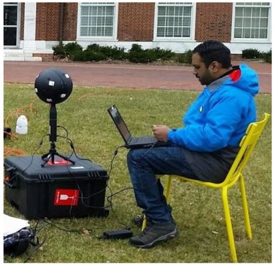
Figure 5. The audiovisual camera used to collect data in a recording session outdoors.

To compute the loudness and location estimate of sound sources in the scene, spherical harmonics beamforming (SHB) technique was used. The 3D sound field sampled at discrete locations on a solid sphere was decomposed into spherical harmonics, whose angular part resolves the direction of the sound field. Spherical harmonics are the 2D counterpart of Fourier transforms (defined on a unit circle) defined on the surface of a sphere. A description of the mathematical details of the SHB method is beyond the scope of this article; interested readers can find details in [67,68,69].

The 64 audio channels recorded at 44,100 Hz were divided into frames, each of 4410 samples. This gave us 10 audio frames per second, which is equal to the video frame rate. Spherical harmonic beamforming was done for the audio frames to locate sounds in the frequency range (300, 6500) Hz. For natural sounds, a wide frequency range as chosen is sufficient to estimate location and loudness of most types of sounds including speech and music. The azimuth angle for SHB was chosen in the range, $[0,2\pi ]$ with the angular resolution of $\frac{2\pi }{128}$ radians, i.e., ${2.8125}^{\circ }$, and the elevation angle in $0,\pi$ with an angular resolution of $\frac{\pi }{64}$ radians, i.e., ${2.8125}^{\mathrm{\circ }}$ radians. The output of SHB is the auditory location and loudness estimate map, as shown in Figure 4.

We collected four audiovisual datasets using the AV camera equipment, where three datasets are 60 s in length and the other is 120 s, all indoors. The AV camera equipment and our algorithms can handle data from any type of audiovisual surroundings, indoor or outdoor. We made sure all combination of salient events in purely visual intensity, color, motion, audio and audiovisual domains were present. SHB was performed with parameters set as explained in the previous paragraph to get the sound location and loudness estimates. The videos were stitched together to produce panoramic image in the Mercator projection, which was used in our saliency computation. The stitch depth for panoramic images was 14 feet; hence, objects that were too close to the AV camera appear to be blurred due to overlapping of images from different cameras on the sphere (Figure 6).

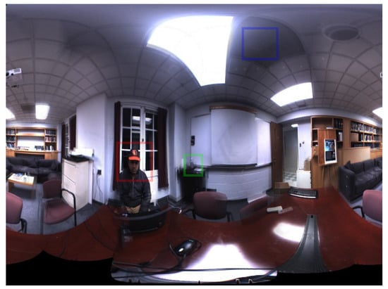
Figure 6. The audiovisual data collection scene. The scene consists of a loudspeaker (green box) and a person and an air conditioning vent (blue box).

The scene consisted of a loudspeaker placed on a desk in one corner of the room (green box) playing documentaries, a person (author) either sitting or moving around the AV camera equipment clapping or uttering numbers out loud, an air conditioning vent (blue box) making some audible noise and other objects visible in the scene. The loudspeaker acts as a stationary sound source, which was switched on/off during the recording session to produce abrupt onsets/offsets. The person wearing a black/blue jacket moving around the recording equipment acts as a salient visual object with or without motion, and when speaking acts as an audiovisual source. The person moves in and out of the room producing abrupt motion onsets/offsets. The air conditioning vent, which happens to be very close to the recording equipment, is a source of noise that is audible to anyone present in the room and acts as another stationary audio source. The bright lights present in the room act as visually salient stationary objects. The set of sources together produce all possible combinations of visually salient events with or without motion, acoustically salient sources with or without motion and audiovisual salient events/objects with and without motion. The dataset can be viewed/listened to at the following url: https://preview.tinyurl.com/ybg4fch4. The results of audiovisual saliency and a comparison with unisensory saliencies on this dataset are discussed in the next section.

5. Results and Discussion

First, we examine which of the three audiovisual saliency computation methods described in Section 3.6, Equations (8)–(10), performs well for different stimulus conditions. Then, we compare results from the best AVSM with the unisensory saliency maps followed by discussion of the results.

All saliency maps computed as explained in Section 3.6 have salience values in $(0,1)$ range. On such a saliency map, unisensory or audiovisual, anything above a threshold of 0.75 is determined as highly salient. This threshold is the same for all saliency maps, visual saliency map ($\mathcal{VSM}$, variables $(x,y,t)$ dropped as unnecessary here), auditory saliency map ($\mathcal{ASM}$) and the three different audiovisual saliency maps (${\mathcal{AVSM}}_i,\mathrm{where}i=1,2,3$). Hence, this provides a common baseline to compare the workings of unisensory SMs with AVSM, and among different AVSMs.

To visualize the results, we did the following: On the saliency map (can be $\mathcal{VSM}$, $\mathcal{ASM}$ or ${\mathcal{AVSM}}_i$), saliency value-based isocontours for the threshold of 0.75 are drawn and superimposed on each of the input video frame. For example, in Figure 7, ${\mathcal{AVSM}}_1$ for Frame #77 of Dataset 2 is shown. Any thing that is inside the closed red contour of Figure 7B is highly salient and has a saliency value greater than 0.75. Outside the isocontour, the salience value is less than 0.75. Exactly along the isocontour, the salience value is 0.75 (precisely, $0.75\pm 0.02$).

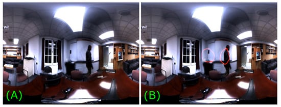
Figure 7. Visualization of results with isocontours: (A) input Frame #77 of Dataset 2; and (B) the red contour superimposed on the same input frame is the isocontour of salience values. All values along the red line are equal to the threshold value. Anything inside the closed red isocontour has a salience value greater than 0.75.

The results can be best interpreted by watching the input and different saliency map videos. However, since it is not possible to show all the frames and for the lack of a better way of presenting the results, we display the saliency maps for a few key frames only. The videos and individual frames of the saliency maps are available at the url: https://preview.tinyurl.com/ybg4fch4.

Figure 8 shows ${\mathcal{AVSM}}_1$, ${\mathcal{AVSM}}_2$ and ${\mathcal{AVSM}}_3$ for input image Frame #393 of Dataset 1. At that moment in the scene, the loudspeaker (at the center of the image frame) was playing a documentary and the person was moving forward. Thus, there is a salient stationary auditory event and a salient visual motion. From visual inspection of Figure 8, it is clear that ${\mathcal{AVSM}}_1$, ${\mathcal{AVSM}}_2$ and ${\mathcal{AVSM}}_3$ give roughly the same results and are able to detect salient events in both modalities. This is the behavior we see in all AVSMs (${\mathcal{AVSM}}_i$) for a majority of frames. However, in some cases, when the scene reduces to a static image, the behavior exhibited by each of the methods will be somewhat different.

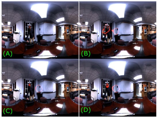
Figure 8. Comparison of audiovisual saliency computation methods. (A) Input Frame #393 of Dataset 1. A small loudspeaker at the corner of a room, which is located almost at the center of the image frame, is playing a documentary, hence constitutes a salient stationary auditory event. The person is leaning forward gives rise to salient visual motion. (B) ${\mathcal{AVSM}}_1$ computed using Equation (8) where all five feature channels are combined linearly with equal weights. (C) ${\mathcal{AVSM}}_2$ computed using Equation (9) where $\mathcal{VSM}$ and $\mathcal{ASM}$ are averaged. (D) ${\mathcal{AVSM}}_3$ computed using Equation (10). All methods give similar results with minor differences

Consider, for example, Frame #173 of Dataset 3, where the visual scene is equivalent to a static image with a weak auditory stimulus, which is the air conditioning vent noise (Figure 9). Here, according to ${\mathcal{AVSM}}_1$ (Figure 9B), the most salient location coincides with the strongest intensity-based salient location at the bottom part of the image. This is because in ${\mathcal{AVSM}}_1$ we averaged the conspicuity maps with equal weights. Thus, when salient audio or motion is not present, the AVSM automatically switches to being a static saliency map with color, intensity and orientation as dominant features. However, in ${\mathcal{AVSM}}_2$, it is computed as the average of visual and auditory saliency maps, hence it leads to redistribution of weights in such a way that each of the visual features contributes only one-eighth to the final saliency map and audio channel contributes one half. As a result, auditory reflections could be accentuated and show up as salient, which may not match with our judgment, as seen in Figure 9C. In reality, such auditory reflections are imperceptible, hence may not draw our attention, as indicated by ${\mathcal{AVSM}}_2$.

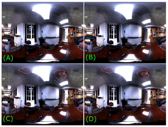
Figure 9. Audiovisual saliency in a static scene. (A) Input Frame #173 of Dataset 3. The scene is almost still reducing the visual input to a static image with a weak auditory noise emanating from the air conditioning vent. (B) The most salient location according to ${\mathcal{AVSM}}_1$ coincides with the intensity-based salient location at the bottom of the image. (C) ${\mathcal{AVSM}}_2$ shows some locations that are not salient according to any feature. This may be happening due to exaggeration of auditory reflections, which are detected as salient in ${\mathcal{AVSM}}_2$. (D) ${\mathcal{AVSM}}_3$ shows similar results as ${\mathcal{AVSM}}_2$.

${\mathcal{AVSM}}_3$, where a multiplicative term, $\mathcal{VSM}(x,y,t)\times \mathcal{ASM}(x,y,t)$, is added, accentuates the conjunction of visual and auditory salient events if they are spatiotemporally coincident. However, since auditory and visual saliencies already contribute equally instead of the five independent features making equal contributions, the effect of the multiplicative term is small, thus we see that ${\mathcal{AVSM}}_3$ has similar behavior as ${\mathcal{AVSM}}_2$. We did not investigate whether the conjunction of individual feature conspicuity maps, e.g. $\mathcal{I}(x,y,t)\times \mathcal{ASM}(x,y,t)$, $\mathcal{O}(x,y,t)\times \mathcal{C}(x,y,t)$, etc. can result in a better saliency map. However, based on visual comparison, we can conclude that ${\mathcal{AVSM}}_1$, where each feature channel contributes equally, irrespective of whether it is visual or auditory, is a better AVSM computation method compared to ${\mathcal{AVSM}}_2$ and ${\mathcal{AVSM}}_3$.

Thus, an important observation we can make at this point is that, even though vision and audition are two separate sensory modalities and we expect them to equally influence the bottom-up, stimulus driven attention, this may not be the case. Instead, we can conclude that each feature irrespective of the sensory modality makes the same contribution to the final saliency map from a bottom-up perspective.

Next, we compare how ${\mathcal{AVSM}}_1$ performs in comparison to unisensory saliency maps, namely $\mathcal{VSM}$ and $\mathcal{ASM}$. Since ${\mathcal{AVSM}}_1$ was found to be better, the other two AVSMs are not discussed.

Figure 10 shows $\mathcal{ASM}$, $\mathcal{VSM}$ and ${\mathcal{AVSM}}_1$ for Frame #50 of Dataset 4, where the person moving is the most salient event, which is correctly detected in $\mathcal{VSM}$ and ${\mathcal{AVSM}}_1$, but not in $\mathcal{ASM}$. This is expected.

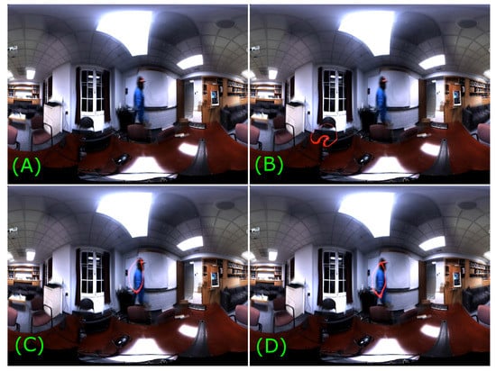
Figure 10. Comparison of AVSM with unisensory saliency maps. (A) Input Frame #50 of Dataset 4. The most prominent event in the scene is the person moving. (B) The most salient location according to $\mathcal{ASM}$ misses the most salient location, but shows a different location as salient. (C) $\mathcal{VSM}$ shows the prominent motion event as salient as expected. (D) ${\mathcal{AVSM}}_1$ also captures the salient motion event as the most salient.

Next, in Figure 11, saliency maps for Frame #346 of Dataset 2 are shown, where audio from the loudspeaker is the most salient event, which is correctly detected as salient in $\mathcal{ASM}$ and ${\mathcal{AVSM}}_1$ but missed in $\mathcal{VSM}$, which agrees with our judgment.

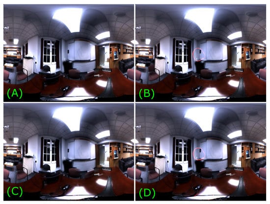
Figure 11. Comparison of AVSM with unisensory saliency maps. (A) Input Frame #346 of Dataset 2. The most prominent event in the scene is the audio from the loudspeaker. (B) The audio event is salient in $\mathcal{ASM}$. (C) $\mathcal{VSM}$ in this case would be equivalent to a static saliency map, hence the auditory salient event is missed here. (D) ${\mathcal{AVSM}}_1$ also captures the audio as the most salient as expected.

In Frame #393 of Dataset 1, there is strong motion of the person as well as sound from the loudspeaker. The unisensory and audiovisual saliency maps are shown in Figure 12. Again, the salients events detected by the respective saliency maps agree with our judgment.

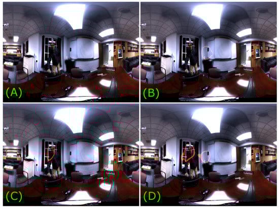
Figure 12. Comparison of AVSM with unisensory saliency maps: (A) input Frame #393 of Dataset 1; (B) $\mathcal{ASM}$ detects the salient auditory event, but misses the salient visual motion; (C) $\mathcal{VSM}$ correctly detects the salient motion event, but misses the salient audio; and (D) ${\mathcal{AVSM}}_1$ captures both valid salient events from two different sensory domains.

From these results, we can conclude that the unisensory saliency maps detect valid unisensory events which agree with human judgment. At the same time, the audiovisual saliency map detects salient events from both sensory modalities, which again agree with our judgment. Thus, we can say, the AVSM detects more number of valid salient events compared to unisensory saliency maps. The unisensory saliency maps miss the salient events from the other sensory modality. Hence, AVSMs in general, and ${\mathcal{AVSM}}_1$ in particular, perform better than unisensory saliency maps in detecting valid salient events. As a result, AVSMs can be more useful in a variety of applications such as surveillance, robotic navigation, etc. Overall, the proto-object-based audiovisual saliency map reliably detects valid salient events for all combinations of auditory, visual and audiovisual events in a majority of the frames. The readers can verify themselves additionally by watching the videos or looking at individual video frames at: https://preview.tinyurl.com/ybg4fch4.

An important distinguishing factor of our AVSM computation comes from the use of proto-objects. With proto-object-based computation, we see that salient locations roughly coincide with object centers giving an estimate of audiovisual “objectness” [72]. Thus, this enables selection of image regions with possible objects based on saliency values. Moreover, since saliency gives a natural mechanism for ranking scene locations based on salience value, combined with “objectness" that comes from proto-objects, this can serve to select image regions for object recognition, activity recognition, etc. with other methods, such as deep convolutional neural networks [73,74].

Second, due to linear combination of feature conspicuity maps, the model adapts itself to any scene type, static or dynamic scenes, with or without audio. Because of this, we get a robust estimate of bottom-up saliency in a majority of cases. In addition, the method works well for a variety of environments, indoor and outdoor.

Finally, the AVSM computed in this manner enables us to represent and compare saliencies of events from two different sensory modalities on a common scale. Other sensory modalities or feature channels can be similarly incorporated into the model.

One of the factors that we have not considered in our model is the temporal modulation of audiovisual saliency. We treat each 100-ms interval as a snapshot, independent of previous frames and compute unisensory and audiovisual saliencies for each 100-ms frame. Even though this “memoryless” computation detects valid salient events well, temporal aspects are found to strongly influence saliency, especially from the auditory domain [75]. Hence, factoring in the temporal dependence of saliency can further improve the model. For example, in the few cases where saliency maps appears to be noisy, we can improve the results with temporal smoothing of the saliency maps. However, the proportion of such noisy frames is very small compared to valid detections.

Temporal dependence of attention is important from the perspective of perception as well. For example, a continuous motion or an auditory alarm can be salient at the beginning of the event due to abrupt onset, but, if it continues to persist, we may switch our attention to some other event, even though it is prominent in the scene. The mechanism and time course of multisensory attentional modulation needs to be further investigated and incorporated into the model.

Another aspect, related to temporal modulation of audiovisual saliency that we have not considered, is the inhibition of return (IOR) [71,76]. IOR refers to increased reaction time to attend to a previously cued spatial location compared to an uncued location. The exact nature of IOR in the case of audiovisual attention is an active topic of research [77,78]. More recent experimental evidence [77] suggests that IOR is not observed in audiovisual attention conditions. If this is the case, not having audiovisual IOR may not be a significantly limiting factor, but certainly worth investigating.

One drawback of our work is that the results are not validated with human psychophysics experiments. Since saliency models aim to predict human attention based on bottom-up features, validating the results with human psychophysics experiments is necessary. Such validation would strengthen the findings of our study even more. Collecting psychophysics data for model validation is challenging because: (i) our data are 360${}^{\circ }$ in both visual and auditory domains, whereas human vision is limited to only 220${}^{\circ }$ (including peripheral vision), hence it necessitates collecting data in a coordinated fashion about other orienting behaviors such as torso movement, head movement, etc.; and (ii) re-creating spatial audio for human rendering comes with its own challenges since the pinna of human ear is uniquely shaped for each individual. Hence, doing a scientifically accurate validation of this perceptual model is beyond the scope of this paper. One might argue that we can draw bounding boxes around salient events and use that as ground-truth for validation. Given that perceptual processes are fast (on the order of milliseconds) and that the translation of what is perceived by the motor system takes considerably higher amount of time, such an experimental design would not be scientifically accurate because it introduces additional influencing variables. Even though we initially considered such a method for validation, we later we dropped the idea and instead focused on a more scientifically accurate method of validation. As we continue to collect experimental data, we would like to present psychophysics validation of the model as soon as possible. However, from visual judgment of the results presented in this work, the readers can verify that the model is capable of selecting valid, perceptually salient audiovisual events for further processing. Moreover, our goal is to build a useful computational tool for automated scene analysis and the results show that the model is capable of doing so.

Lastly, we could not compare the performance of the model with other methods. This is because most audiovisual saliency models do not incorporate spatial aspects of audio such as loudness and location. Moreover, comparing with other models requires psychophysics experimental data, which are not available now. In the future, we would like to compare the performance of our model against other spatiotemporal AV saliency models.

6. Conclusions and Future Work

We show that a proto-object-based audiovisual saliency map detects salient unisensory and multisensory events, which agree with human judgment. The AVSM detects a higher number of valid salient events compared to unisensory saliency maps, demonstrating the superiority and usefulness of proto-object-based multisensory saliency maps. Among the different audiovisual saliency methods, we show that linear combination of individual feature channels with equal weights gives the best results. The AVSM computed this way performs better compared to others in detecting valid salient events for static as well as dynamic scenes, with or without salient auditory events in the scene. In addition, it is less noisy and more robust compared to other combination methods where visual and auditory conspicuity maps, instead of individual feature channels, are equally weighed.

In the future, incorporating the temporal modulation of saliency will be considered. We would also like to validate the AVSM with psychophysics experiments. In addition, the role of Inhibition of Return in the case of an audiovisual saliency map will also be investigated. In conclusion, a proto-object-based audiovisual saliency map with linear and equally weighted feature channels detects a higher number of valid unisensory and multisensory events that agree with human judgment.

MDPI stays neutral with regard to jurisdictional claims in published maps and institutional affiliations.

References

- Stein, B.E.; Stanford, T.R. Multisensory integration: Current issues from the perspective of the single neuron. Nat. Rev. Neurosci. 2008, 9, 255–266. [Google Scholar] [CrossRef] [PubMed]
- Stevenson, R.A.; James, T.W. Audiovisual integration in human superior temporal sulcus: Inverse effectiveness and the neural processing of speech and object recognition. Neuroimage 2009, 44, 1210–1223. [Google Scholar] [CrossRef] [PubMed]
- Calvert, G.A.; Spence, C.; Stein, B.E. The Handbook of Multisensory Processes; MIT Press: Cambridge, MA, USA, 2004. [Google Scholar]
- Spence, C.; Senkowski, D.; Röder, B. Crossmodal processing. Exp. Brain Res. 2009, 198, 107–111. [Google Scholar] [CrossRef] [PubMed]
- Alais, D.; Burr, D. The ventriloquist effect results from near-optimal bimodal integration. Curr. Biol. 2004, 14, 257–262. [Google Scholar] [CrossRef] [PubMed]
- Ghazanfar, A.A.; Schroeder, C.E. Is neocortex essentially multisensory? Trends Cogn. Sci. 2006, 10, 278–285. [Google Scholar] [CrossRef] [PubMed]
- Von Kriegstein, K.; Kleinschmidt, A.; Sterzer, P.; Giraud, A.L. Interaction of face and voice areas during speaker recognition. J. Cogn. Neurosci. 2005, 17, 367–376. [Google Scholar] [CrossRef]
- Watkins, S.; Shams, L.; Tanaka, S.; Haynes, J.D.; Rees, G. Sound alters activity in human V1 in association with illusory visual perception. Neuroimage 2006, 31, 1247–1256. [Google Scholar] [CrossRef]
- Van Wassenhove, V.; Grant, K.W.; Poeppel, D. Visual speech speeds up the neural processing of auditory speech. Proc. Natl. Acad. Sci. USA 2005, 102, 1181–1186. [Google Scholar] [CrossRef]
- Ghazanfar, A.A.; Maier, J.X.; Hoffman, K.L.; Logothetis, N.K. Multisensory integration of dynamic faces and voices in rhesus monkey auditory cortex. J. Neurosci. 2005, 25, 5004–5012. [Google Scholar] [CrossRef] [PubMed]
- Wang, Y.; Celebrini, S.; Trotter, Y.; Barone, P. Visuo-auditory interactions in the primary visual cortex of the behaving monkey: Electrophysiological evidence. BMC Neurosci. 2008, 9, 79. [Google Scholar] [CrossRef]
- Kimchi, R.; Yeshurun, Y.; Cohen-Savransky, A. Automatic, stimulus-driven attentional capture by objecthood. Psychon. Bull. Rev. 2007, 14, 166–172. [Google Scholar] [CrossRef]
- Nuthmann, A.; Henderson, J.M. Object-based attentional selection in scene viewing. J. Vis. 2010, 10, 20. [Google Scholar] [CrossRef] [PubMed]
- Russell, A.F.; Mihalaş, S.; von der Heydt, R.; Niebur, E.; Etienne-Cummings, R. A model of proto-object based saliency. Vis. Res. 2014, 94, 1–15. [Google Scholar] [CrossRef]
- Çetingül, H.; Erzin, E.; Yemez, Y.; Tekalp, A.M. Multimodal speaker/speech recognition using lip motion, lip texture and audio. Signal Process. 2006, 86, 3549–3558. [Google Scholar] [CrossRef]
- Tamura, S.; Iwano, K.; Furui, S. Toward robust multimodal speech recognition. In Symposium on Large Scale Knowledge Resources (LKR2005); Tokyo Tech Research Repository: Tokyo, Japan, 2005; pp. 163–166. [Google Scholar]
- Alais, D.; Newell, F.N.; Mamassian, P. Multisensory processing in review: From physiology to behaviour. Seeing Perceiving 2010, 23, 3–38. [Google Scholar] [CrossRef]
- Meredith, M.A.; Stein, B.E. Visual, auditory, and somatosensory convergence on cells in superior colliculus results in multisensory integration. J. Neurophysiol. 1986, 56, 640–662. [Google Scholar] [CrossRef] [PubMed]
- Evangelopoulos, G.; Rapantzikos, K.; Potamianos, A.; Maragos, P.; Zlatintsi, A.; Avrithis, Y. Movie summarization based on audiovisual saliency detection. In Proceedings of the 2008 15th IEEE International Conference on Image Processing, San Diego, CA, USA, 12–15 October 2008; pp. 2528–2531. [Google Scholar]
- Song, G. Effet du Son Dans Les Vidéos Sur la Direction du Regard: Contribution à la Modélisation de la Saillance Audiovisuelle. Ph.D. Thesis, Université de Grenoble, Saint-Martin-d’Hères, France, 2013. [Google Scholar]
- Ramenahalli, S.; Mendat, D.R.; Dura-Bernal, S.; Culurciello, E.; Nieburt, E.; Andreou, A. Audio-visual saliency map: Overview, basic models and hardware implementation. In Proceedings of the 2013 47th Annual Conference on Information Sciences and Systems (CISS), Baltimore, MD, USA, 20–22 March 2013; pp. 1–6. [Google Scholar]
- Grossberg, S.; Roberts, K.; Aguilar, M.; Bullock, D. A neural model of multimodal adaptive saccadic eye movement control by superior colliculus. J. Neurosci. 1997, 17, 9706–9725. [Google Scholar] [CrossRef] [PubMed]
- Meredith, M.A.; Stein, B.E. Spatial determinants of multisensory integration in cat superior colliculus neurons. J. Neurophysiol. 1996, 75, 1843–1857. [Google Scholar] [CrossRef]
- Meredith, M.A.; Nemitz, J.W.; Stein, B.E. Determinants of multisensory integration in superior colliculus neurons. I. Temporal factors. J. Neurosci. 1987, 7, 3215–3229. [Google Scholar] [CrossRef]
- Casey, M.C.; Pavlou, A.; Timotheou, A. Audio-visual localization with hierarchical topographic maps: Modeling the superior colliculus. Neurocomputing 2012, 97, 344–356. [Google Scholar] [CrossRef]
- Huo, J.; Murray, A. The adaptation of visual and auditory integration in the barn owl superior colliculus with Spike Timing Dependent Plasticity. Neural Netw. 2009, 22, 913–921. [Google Scholar] [CrossRef]
- Huo, J.; Murray, A.; Wei, D. Adaptive visual and auditory map alignment in barn owl superior colliculus and its neuromorphic implementation. IEEE Trans. Neural Netw. Learn. Syst. 2012, 23, 1486–1497. [Google Scholar] [PubMed]
- Anastasio, T.J.; Patton, P.E.; Belkacem-Boussaid, K. Using Bayes’ rule to model multisensory enhancement in the superior colliculus. Neural Comput. 2000, 12, 1165–1187. [Google Scholar] [CrossRef]
- Patton, P.; Belkacem-Boussaid, K.; Anastasio, T.J. Multimodality in the superior colliculus: An information theoretic analysis. Cogn. Brain Res. 2002, 14, 10–19. [Google Scholar] [CrossRef]
- Patton, P.E.; Anastasio, T.J. Modeling cross-modal enhancement and modality-specific suppression in multisensory neurons. Neural Comput. 2003, 15, 783–810. [Google Scholar] [CrossRef] [PubMed]
- Colonius, H.; Diederich, A. Why aren’t all deep superior colliculus neurons multisensory? A Bayes’ ratio analysis. Cogn. Affect. Behav. Neurosci. 2004, 4, 344–353. [Google Scholar] [CrossRef] [PubMed][Green Version]
- Ma, W.J.; Beck, J.M.; Latham, P.E.; Pouget, A. Bayesian inference with probabilistic population codes. Nat. Neurosci. 2006, 9, 1432–1438. [Google Scholar] [CrossRef]
- Wilson, K.; Rangarajan, V.; Checka, N.; Darrell, T. Audiovisual Arrays for Untethered Spoken Interfaces. In Proceedings of the 4th IEEE International Conference on Multimodal Interfaces, Pittsburgh, PA, USA, 16 October 2002; IEEE Computer Society: Washington, DC, USA, 2002; pp. 389–394. [Google Scholar]
- Torres, F.; Kalva, H. Influence of audio triggered emotional attention on video perception. In Human Vision and Electronic Imaging XIX; International Society for Optics and Photonics: Bellingham, WA, USA, 2014; p. 901408. [Google Scholar]
- Lee, J.S.; De Simone, F.; Ebrahimi, T. Efficient video coding based on audio-visual focus of attention. J. Vis. Commun. Image Represent. 2011, 22, 704–711. [Google Scholar] [CrossRef]
- Rerabek, M.; Nemoto, H.; Lee, J.S.; Ebrahimi, T. Audiovisual focus of attention and its application to Ultra High Definition video compression. In Human Vision and Electronic Imaging XIX; International Society for Optics and Photonics: Bellingham, WA, USA, 2014; p. 901407. [Google Scholar]
- Ruesch, J.; Lopes, M.; Bernardino, A.; Hornstein, J.; Santos-Victor, J.; Pfeifer, R. Multimodal saliency-based bottom-up attention a framework for the humanoid robot icub. In Proceedings of the IEEE International Conference on Robotics and Automation, Pasadena, CA, USA, 19–23 May 2008; pp. 962–967. [Google Scholar]
- Schauerte, B.; Richarz, J.; Plötz, T.; Thurau, C.; Fink, G.A. Multi-modal and multi-camera attention in smart environments. In Proceedings of the 2009 International Conference on Multimodal Interfaces, Cambridge, MA, USA, 2–4 November 2009; ACM: New York, NY, USA, 2009; pp. 261–268. [Google Scholar]
- Schauerte, B.; Kuhn, B.; Kroschel, K.; Stiefelhagen, R. Multimodal saliency-based attention for object-based scene analysis. In Proceedings of the IEEE/RSJ International Conference on Intelligent Robots and Systems, San Francisco, CA, USA, 25–30 September 2011; pp. 1173–1179. [Google Scholar]
- Schauerte, B. Bottom-Up Audio-Visual Attention for Scene Exploration. In Multimodal Computational Attention for Scene Understanding and Robotics; Springer: Berlin/Heidelberg, Germany, 2016; pp. 35–113. [Google Scholar]
- Onat, S.; Libertus, K.; Konig, P. Integrating audiovisual information for the control of overt attention. J. Vis. 2007, 7, 11. [Google Scholar] [CrossRef][Green Version]
- Kühn, B.; Schauerte, B.; Stiefelhagen, R.; Kroschel, K. A modular audio-visual scene analysis and attention system for humanoid robots. In Proceedings of the 43rd International Symposium on Robotics (ISR), Taipei, Taiwan, 29–31 August 2012. [Google Scholar]
- Kühn, B.; Schauerte, B.; Kroschel, K.; Stiefelhagen, R. Multimodal saliency-based attention: A lazy robot’s approach. In Proceedings of the IEEE/RSJ International Conference on Intelligent Robots and Systems, Vilamoura, Portugal, 7–12 October 2012; pp. 807–814. [Google Scholar]
- Bauer, J.; Weber, C.; Wermter, S. A SOM-based model for multi-sensory integration in the superior colliculus. In Proceedings of the 2012 International Joint Conference on Neural Networks (IJCNN), Brisbane, Australia, 10–15 June 2012; pp. 1–8. [Google Scholar]
- Viciana-Abad, R.; Marfil, R.; Perez-Lorenzo, J.M.; Bandera, J.P.; Romero-Garces, A.; Reche-Lopez, P. Audio-Visual perception system for a humanoid robotic head. Sensors 2014, 14, 9522–9545. [Google Scholar] [CrossRef]
- Evangelopoulos, G.; Rapantzikos, K.; Maragos, P.; Avrithis, Y.; Potamianos, A. Audiovisual attention modeling and salient event detection. In Multimodal Processing and Interaction; Springer: Berlin/Heidelberg, Germany, 2008; pp. 1–21. [Google Scholar]
- Rapantzikos, K.; Evangelopoulos, G.; Maragos, P.; Avrithis, Y. An Audio-Visual Saliency Model for Movie Summarization. In Proceedings of the 2007 IEEE 9th Workshop on Multimedia Signal Processing, Crete, Greece, 1–3 October 2007; pp. 320–323. [Google Scholar]
- Evangelopoulos, G.; Zlatintsi, A.; Potamianos, A.; Maragos, P.; Rapantzikos, K.; Skoumas, G.; Avrithis, Y. Multimodal saliency and fusion for movie summarization based on aural, visual, and textual attention. IEEE Trans. Multimed. 2013, 15, 1553–1568. [Google Scholar] [CrossRef]
- Nakajima, J.; Sugimoto, A.; Kawamoto, K. Incorporating audio signals into constructing a visual saliency map. In Image and Video Technology; Springer: Berlin/Heidelberg, Germany, 2014; pp. 468–480. [Google Scholar]
- Itti, L.; Baldi, P. Bayesian surprise attracts human attention. Vis. Res. 2009, 49, 1295–1306. [Google Scholar]
- Nakajima, J.; Kimura, A.; Sugimoto, A.; Kashino, K. Visual Attention Driven by Auditory Cues. In MultiMedia Modeling; Springer: Berlin/Heidelberg, Germany, 2015; pp. 74–86. [Google Scholar]
- Korchagin, D.; Motlicek, P.; Duffner, S.; Bourlard, H. Just-in-time multimodal association and fusion from home entertainment. In Proceedings of the 2011 IEEE International Conference on Multimedia and Expo (ICME), Barcelona, Spain, 11–15 July 2011; pp. 1–5. [Google Scholar]
- Hershey, J.R.; Movellan, J.R. Audio Vision: Using Audio-Visual Synchrony to Locate Sounds. In Advances in Neural Information Processing Systems; MIT Press: Cambridge, MA, USA, 2000; pp. 813–819. [Google Scholar]
- Blauth, D.A.; Minotto, V.P.; Jung, C.R.; Lee, B.; Kalker, T. Voice activity detection and speaker localization using audiovisual cues. Pattern Recognit. Lett. 2012, 33, 373–380. [Google Scholar]
- Ratajczak, R.; Pellerin, D.; Labourey, Q.; Garbay, C. A Fast Audiovisual Attention Model for Human Detection and Localization on a Companion Robot. In Proceedings of the First International Conference on Applications and Systems of Visual Paradigms (VISUAL 2016), Barcelona, Spain, 13–17 November 2016. [Google Scholar]
- Song, G.; Pellerin, D.; Granjon, L. How different kinds of sound in videos can influence gaze. In Proceedings of the 13th International Workshop on Image Analysis for Multimedia Interactive Services (WIAMIS), Dublin, Ireland, 23–25 May 2012; pp. 1–4. [Google Scholar]
- Coutrot, A.; Guyader, N. How saliency, faces, and sound influence gaze in dynamic social scenes. J. Vis. 2014, 14, 5. [Google Scholar]
- Coutrot, A.; Guyader, N. An audiovisual attention model for natural conversation scenes. In Proceedings of the IEEE International Conference on Image Processing (ICIP), Paris, France, 27–30 October 2014; pp. 1100–1104. [Google Scholar]
- Sidaty, N.O.; Larabi, M.C.; Saadane, A. Towards Understanding and Modeling Audiovisual Saliency Based on Talking Faces. In Proceedings of the Tenth International Conference on Signal-Image Technology and Internet-Based Systems (SITIS), Marrakech, Morocco, 23–27 November 2014; pp. 508–515. [Google Scholar]
- Min, X.; Zhai, G.; Zhou, J.; Zhang, X.P.; Yang, X.; Guan, X. A multimodal saliency model for videos with high audio-visual correspondence. IEEE Trans. Image Process. 2020, 29, 3805–3819. [Google Scholar]
- Tavakoli, H.R.; Borji, A.; Kannala, J.; Rahtu, E. Deep Audio-Visual Saliency: Baseline Model and Data. In Proceedings of the Symposium on Eye Tracking Research and Applications, Stuttgart, Germany, 2–5 June 2020; Association for Computing Machinery: New York, NY, USA, 2020; pp. 1–5. [Google Scholar]
- Tsiami, A.; Koutras, P.; Maragos, P. STAViS: Spatio-Temporal AudioVisual Saliency Network. In Proceedings of the IEEE/CVF Conference on Computer Vision and Pattern Recognition, Seattle, WA, USA, 14–19 June 2020; pp. 4766–4776. [Google Scholar]
- Koutras, P.; Panagiotaropoulou, G.; Tsiami, A.; Maragos, P. Audio-visual temporal saliency modeling validated by fmri data. In Proceedings of the IEEE Conference on Computer Vision and Pattern Recognition Workshops, Salt Lake City, UT, USA, 18–22 June 2018; pp. 2000–2010. [Google Scholar]
- Rensink, R.A. The dynamic representation of scenes. Vis. Cogn. 2000, 7, 17–42. [Google Scholar]
- Sun, D.; Roth, S.; Black, M.J. Secrets of optical flow estimation and their principles. In Proceedings of the 2010 IEEE Conference on Computer Vision and Pattern Recognition (CVPR), San Francisco, CA, USA, 13–18 June 2010; pp. 2432–2439. [Google Scholar]
- Sun, D.; Roth, S.; Black, M. Optic Flow Estimation MATLAB Code. 2008. Available online: http://cs.brown.edu/~dqsun/code/cvpr10_flow_code.zip (accessed on 2 November 2020).
- Donovan, A.O.; Duraiswami, R.; Neumann, J. Microphone arrays as generalized cameras for integrated audio visual processing. In Proceedings of the IEEE Conference on Computer Vision and Pattern Recognition, Minneapolis, MN, USA, 17–22 June 2007; pp. 1–8. [Google Scholar]
- Meyer, J.; Elko, G. A highly scalable spherical microphone array based on an orthonormal decomposition of the soundfield. In Proceedings of the IEEE International Conference on Acoustics, Speech, and Signal Processing (ICASSP), Orlando, FL, USA, 13–17 May 2002; Volume 2, p. II–1781. [Google Scholar]
- O’Donovan, A.; Duraiswami, R.; Gumerov, N. Real time capture of audio images and their use with video. In Proceedings of the IEEE Workshop on Applications of Signal Processing to Audio and Acoustics, New Paltz, NY, USA, 21–24 October 2007; pp. 10–13. [Google Scholar]
- Zhang, N.; von der Heydt, R. Analysis of the context integration mechanisms underlying figure–ground organization in the visual cortex. J. Neurosci. 2010, 30, 6482–6496. [Google Scholar] [CrossRef] [PubMed]
- Itti, L.; Koch, C.; Niebur, E. A model of saliency-based fast visual attention for rapid scene analysis. IEEE Trans. Pattern Anal. Mach. Intell. 1998, 20, 1254–1259. [Google Scholar]
- Alexe, B.; Deselaers, T.; Ferrari, V. Measuring the objectness of image windows. IEEE Trans. Pattern Anal. Mach. Intell. 2012, 34, 2189–2202. [Google Scholar]
- Krizhevsky, A.; Sutskever, I.; Hinton, G.E. Imagenet classification with deep convolutional neural networks. In Proceedings of the Advances in Neural Information Processing Systems 25: 26th Annual Conference on Neural Information Processing Systems 2012, Lake Tahoe, NV, USA, 3–6 December 2012; pp. 1097–1105. [Google Scholar]
- Ren, S.; He, K.; Girshick, R.; Sun, J. Faster R-CNN: Towards real-time object detection with region proposal networks. In Proceedings of the Advances in Neural Information Processing Systems 28 (NIPS 2015), Montreal, QC, Canada, 7–12 December 2015; pp. 91–99. [Google Scholar]
- Kaya, E.M.; Elhilali, M. A temporal saliency map for modeling auditory attention. In Proceedings of the 2012 46th Annual Conference on Information Sciences and Systems (CISS), Princeton, NJ, USA, 21–23 March 2012; pp. 1–6. [Google Scholar]
- Posner, M.I.; Cohen, Y. Components of visual orienting. In Attention and Performance X: Control of Language Processes; Bouma, H., Bouwhuis, D.G., Eds.; Psychology Press: East Sussex, UK, 1984; pp. 531–556. [Google Scholar]
- Van der Stoep, N.; Van der Stigchel, S.; Nijboer, T.; Spence, C. Visually Induced Inhibition of Return Affects the Integration of Auditory and Visual Information. Perception 2017, 46, 6–17. [Google Scholar] [CrossRef] [PubMed]
- Spence, C.; Driver, J. Auditory and audiovisual inhibition of return. Atten. Percept. Psychophys. 1998, 60, 125–139. [Google Scholar] [CrossRef]
Publisher’s Note: MDPI stays neutral with regard to jurisdictional claims in published maps and institutional affiliations. |
© 2020 by the author. Licensee MDPI, Basel, Switzerland. This article is an open access article distributed under the terms and conditions of the Creative Commons Attribution (CC BY) license (http://creativecommons.org/licenses/by/4.0/).