Toward Smart School Mobility: IoT-Based Comfort Monitoring Through Sensor Fusion and Standardized Signal Analysis

Abstract

As smart cities evolve, integrating new technologies into school transportation is becoming increasingly important to ensure student comfort and safety. Monitoring and enhancing comfort during daily commutes can significantly influence well-being and learning readiness. However, most existing research addresses isolated factors, which limits the development of comprehensive and scalable solutions. This study presents the design and implementation of a low-cost, generalized IoT-based system for monitoring comfort in school transportation. The system processes multiple environmental and operational signals, and these data are transmitted to a cloud computing platform for real-time analysis. Signal processing incorporates standardized metrics, such as root mean square (RMS) values from ISO 2631-1 for vibration assessment. In addition, machine learning techniques, including a Random Forest classifier and ensemble-based models, are applied to classify ride comfort levels using both road roughness and environmental variables. The results show that stacked multisensor fusion achieved a significant improvement in classification performance compared with vibration-only models. The platform also integrates route visualization with commuting time per student, providing valuable information to assess the impact of travel duration on school mobility.

1. Introduction

Rapid technological convergence has accelerated the development of smart cities, driven by paradigms such as the Internet of Things (IoT), wireless sensor networks, big data, machine learning, and cloud computing [1,2], and supported by advanced communication technologies including LPWAN, NB-IoT, 4G, 5G, and optical systems [3,4,5]. Within this ecosystem, smart transportation stands out as a particularly impactful application [6], integrating sensors, computing devices, communication infrastructure, and data analytics to improve safety, efficiency, and sustainability in transport networks [7].

This study focuses on van-based school transportation systems, a common mode of commuting that has a direct impact on student well-being, safety, and access to education. Reliable transportation has been shown to be essential for regular school attendance, with limited access associated with increased absenteeism, particularly among younger students [8]. In addition, the mode of transportation can affect the cognitive performance of children, further underscoring the importance of transportation quality [9].

IoT technologies play an important role in the evaluation of transport sustainability, enabling real-time monitoring of safety, congestion, energy consumption, environmental impact, and accessibility [10,11]. Motivated by this vision, the present study proposes a low-cost IoT-based system and architecture to monitor comfort in school transportation [12], thereby overcoming the limitations of traditional approaches that rely primarily on subjective passenger surveys [13]. Comfort in transportation is shaped by multiple psychological, demographic, socioeconomic, and infrastructure factors, yet objective sensor-based monitoring remains scarce. The proposed system addresses this gap by providing real-time comfort assessment using physical signals, while the resulting data platform offers decision support for urban mobility policies, particularly in school transport [14].

Related studies identify mechanical vibrations as the most influential factor in comfort analysis [15], while additional parameters such as temperature, humidity, noise, and speed also play a relevant role [16]. Building on these insights, this work introduces an IoT sensing platform that integrates accelerometers, environmental sensors, noise meters, and GPS modules to derive a comprehensive comfort index from multiple correlated variables, including vibration levels, travel time, and vehicle dynamics.

At the sensing node, a Raspberry Pi 4B serves as the Single-Board Computer (SBC) to enable edge computing. The SBC performs local preprocessing, such as conditioning vibration signals to mitigate aliasing and gravitational effects [17], thus reducing latency and bandwidth before transmission to the cloud. The comfort levels are then evaluated according to the ISO 2631-1 standard for assessing human exposure to mechanical vibrations [15], while the cloud platform supports data visualization, storage, advanced analytics, and automated reporting [18]. Pre-processed sensor signals also serve as input for machine learning models capable of estimating passenger comfort based on vibration and related parameters [16]. Meanwhile, the integrated GPS module provides precise geolocation, vehicle speed, and route data, enabling spatio-temporal mapping of comfort conditions along school journeys.

Field deployment tests demonstrate how these heterogeneous data streams can be combined into a global comfort index, offering a holistic assessment of passenger well-being. The resulting information is visualized in a user-friendly dashboard that supports both real-time monitoring and offline analysis and can trigger alerts when predefined thresholds or abnormal patterns are detected.

The remainder of this paper is organized as follows. Section 2 reviews related work on comfort assessment methodologies. Section 3 details the system architecture, hardware components, and the data processing pipeline. Section 4 presents experimental results from a real-world deployment in a school transportation setting. Section 5 discusses the findings, highlighting their implications and limitations. Finally, Section 6 concludes the paper and outlines future research directions.

2. Ride Comfort Characterization

Ride comfort in public transportation systems is a multifaceted phenomenon influenced by both physical and subjective factors. Quantifiable parameters that significantly affect perceived comfort and can be monitored using IoT-based systems include temperature, humidity, noise levels, vehicle speed, travel time, and, most importantly, vibration. This section reviews established methodologies, parameters, and standardized evaluation criteria commonly employed to assess and quantify ride comfort, according to the parameters evaluated in public transportation environments.

2.1. Thermal Comfort

Thermal comfort is inherently subjective, as it depends on a combination of environmental and personal factors, making it challenging to establish a single universal definition [19]. To address this complexity, standards such as ASHRAE 55 [19] and ISO 7730 [20] propose comfort models that categorize influencing variables into environmental parameters (air temperature, mean radiant temperature, air velocity, and relative humidity) and personal parameters (metabolic rate and clothing insulation). These variables form the basis for the widely used indices Predicted Mean Vote (PMV) and Predicted Percentage of Dissatisfied (PPD), originally developed through Fanger’s experiments [21].

Despite being a widely discussed topic, the adoption of IoT solutions for the assessment of thermal comfort remains limited. Recent studies emphasize the importance of sensor-based systems capable of continuously monitoring comfort parameters and incorporating features such as color schemes or alarms for effective risk communication [22]. To facilitate practical implementation, simplified approaches have been developed, such as reduced versions of the PMV model, which minimize the number of required parameters and allow the estimation of thermal comfort without incurring additional costs or installing specialized sensors [23].

The air temperature is among the simplest parameters to assess within a vehicle cabin, but it is strongly influenced by seasonal variations and the location of the measurement. Comfort is generally reported between 23 °C and 28 °C, although this range can change in hot, humid conditions or under strong solar exposure [24]. Lin et al. [25] found that neutral temperatures in summer ranged from 22.4 °C to 28.9 °C for short-haul vehicles and 22.4 °C to 30.1 °C for long-haul vehicles. Similarly, Velt and Daanen [26] observed that an average in-bus temperature of 22.5  °C was perceived to be slightly warm, suggesting an optimal winter comfort range of 20 °C to 24 °C. However, as discussed earlier, contextual factors, such as cabin size, window, and upholstery, can significantly alter thermal perception [27]. Taken together, these studies suggest that while neutral cabin temperatures generally fall between 22–29 °C in summer and 20–24 °C in winter, perceived comfort is highly dependent on contextual and environmental conditions.

Although traditional sensor-based methods provide valuable insight, they are often costly and limited by test conditions and sensor placement. Computational Fluid Dynamics (CFD) offers a complementary approach that enables computationally efficient simulations that optimize the thermal parameters. Rong et al. [28] investigated thermal comfort and air quality in fully occupied buses using CFD simulations. They applied the PMV index along with the CO₂ concentration as key indicators. Their results recommend maintaining an internal temperature between 20 °C and 28 °C, according to air quality management guidelines, to ensure comfort in air-conditioned public transport.

Complementing simulation-based approaches, several field studies have combined objective and subjective measures to evaluate comfort directly in real transport environments. Davydova et al. [29] assessed thermal comfort in semi-enclosed public transport vehicles on four routes used by university students in Guadalajara, Mexico. The environmental measurements of temperature and humidity were paired with passenger surveys. The Apparent Temperature Index (ATI) predominantly ranged from 30 °C to 38 °C, exceeding established comfort thresholds. Only 23% of the values fell within the comfort range of 20 °C to 28 °C. Using the Fanger PMV/PPD method, the study estimated that 31% of the passengers were thermally dissatisfied, highlighting the frequent occurrence of thermal stress in public transport, particularly during the warmer months of May and October.

2.2. Acoustic Comfort and Noise Levels

According to the Brazilian Ergonomics Standard NR-17 [30], noise levels are considered acoustically comfortable when they are at or below 65 dB(A). Levels that exceed this threshold are classified as uncomfortable. In parallel, the Brazilian Occupational Health Standard NHO-01 specifies that noise exposure between 82 dB(A) to 85 dB(A) necessitates preventive or corrective measures, while levels above 85 dB(A) require immediate mandatory interventions.

Zannin [31] conducted an assessment of occupational noise exposure in urban buses and found that while most vehicles operated below the 82 dB(A) threshold, making them acceptable under NHO-01 guidelines, they still exceeded the comfort threshold defined by NR-17, indicating an uncomfortable environment from an ergonomic perspective.

Portela and Zannin [32] further emphasize the importance of reducing cabin noise levels to enhance acoustic comfort for both drivers and passengers. Although none of the buses studied exceeded the occupational safety limit of 85 dB(A), the majority registered above 65 dB(A), suggesting discomfort. The authors recommend engineering solutions such as moving the engines to the rear and incorporating noise-dampening materials to improve the acoustic environment and promote occupational well-being in public transportation systems.

Silva and Correia [33] conducted a noise exposure assessment in public buses in Itajubá, Brazil. Their study aimed to evaluate both passenger comfort and health risk using World Health Organization (WHO) guidelines as a reference [34]. Noise levels were measured on 15 bus routes for 23 h, showing values between 78 dB(A)and 84 dB(A), with a mean of 81 dB(A). These values significantly exceed the WHO recommended limits for community noise, where discomfort is observed between 50 dB(A) and 55 dB(A) for a period of 16 h, and the risk of hearing damage is associated with 70 dB(A) for 24 h.

2.3. Vibration Exposure and Ride Comfort

Ride comfort is significantly influenced by whole-body vibration and irregularities on road surface. Over the past decades, a range of methodologies have been developed to quantify and improve ride comfort through both objective measurements and subjective feedback.

Zhao et al. [15] introduced a vibration-based method compliant with ISO 2631-1 to evaluate ride comfort in buses. Their approach used smartphones as crowd-sourced sensors to collect vibration data during transit. Through coordinate transformation and low-pass filtering, the method isolated the relevant components of body vibration. The resulting weighted root mean square acceleration ($a_{wT}$) was then converted into a comfort score using a quadratic regression model, allowing real-time passenger feedback through onboard systems.

Griffin and Whitham [35] investigated the effect of exposure duration on the perception of whole-body vibration discomfort. In a controlled laboratory setup, they exposed subjects to alternating 4 Hz and 16 Hz vertical sinusoidal vibrations, applying a discomfort-matching technique. Their results did not reveal a significant variation in relative discomfort over exposure durations up to 36 min. This supports the ISO 2631 assumption that vibration discomfort is predominantly frequency-dependent and does not strongly depend on exposure duration.

Similarly, Castellanos and Fruett [36] developed an embedded system that combines hardware, firmware, and software to monitor dynamic vehicle behavior. Their system measured acceleration and jerk (the rate of change in acceleration) to detect discomfort events and compute a Comfort Index based on ISO 2631-1 guidelines. Their dual-algorithm strategy provided both average comfort metrics and real-time event localization, with on-board user feedback used for threshold calibration.

Zhang et al. [37] presented a comprehensive bus comfort model that integrated both subjective and objective parameters. They evaluated vibration, noise, acceleration, and thermal comfort on urban bus routes in Nanjing, China. Using a combination of onboard data acquisition and passenger surveys, a regression model was developed to quantify Overall Bus Comfort (OBC), showing that vibration and acceleration were dominant contributors to perceived discomfort.

The work of Zhou et al. [38] presents an experimental study that examined the combinations of temperature, noise, and whole-body vibration affect both thermal and overall comfort. Using a factorial design with 24 participants, the authors found that temperature had the strongest influence on thermal comfort, while noise and vibration significantly decreased overall comfort. The results highlight the importance of evaluating multimodal environmental stressors in combination. However, the study was conducted under controlled laboratory conditions and did not explore real-time applications or mobile environments.

2.4. Machine Learning for Ride Quality

Recent studies have increasingly applied machine learning to evaluate road roughness and its correlation with ride comfort, as these methods effectively capture nonlinear relationships among variables. Ajayi et al. [39] analyzed more than one million rows of smartphone sensor data using Random Forest (RF), XGBoost, and Support Vector Regression (SVR). Although XGBoost achieved the highest accuracy, Random Forest was preferred for its robustness, lower memory usage, and suitability for real-time deployment. The study concluded that RF offers the best trade-off between predictive accuracy and computational efficiency to evaluate comfort in long-haul transportation. In related work, Baji et al. [40] proposed a framework to estimate road roughness based on vertical acceleration ($a_z$) and vehicle speed. By applying supervised models such as linear regression and RF, the system was able to predict the International Roughness Index (IRI) with high accuracy, enabling scalable and real-time pavement monitoring.

In a complementary line of research, Chen et al. [41] proposed an Autonomous Driving Comfort Prediction (ADCP) model that integrates XGBoost with a multihead self-attention mechanism to estimate comfort indicators such as jerk and acceleration from road and traffic characteristics. Trained in both real and simulated data sets, the models incorporated factors such as path distance, traffic density, intersections, and weather conditions. Although XGBoost outperformed a baseline neural network, the attention-based model proved more robust under complex driving scenarios, delivering superior comfort prediction in variable conditions. Real-world validation further demonstrated that the incorporation of the ADCP model into path planning reduced jerk and improved subjective comfort scores.

Another significant contribution is that of Al-Refai et al. [42], who developed a low-cost machine learning framework to classify road surface conditions, traffic levels, and driving styles using only data from the vehicle controller area network (CAN). Using standard vehicle sensors and avoiding costly external instrumentation, the system demonstrated strong potential for embedded applications. Among the models tested, the Random Forest classifier achieved the highest precision (up to 95%).

Taken together, these studies illustrate the ongoing evolution of ride comfort assessment, moving beyond direct acceleration-based indices to integrated frameworks that combine user feedback, signal processing, and machine learning to enable real-time comfort assessment and infrastructure monitoring.

3. Materials and Methods

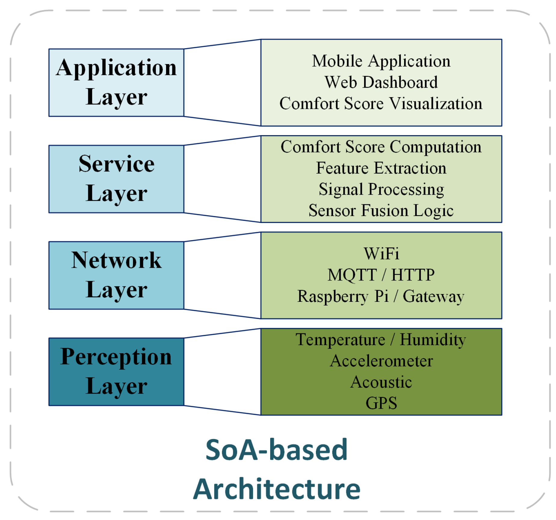
This section presents the materials and methods used to compute the comfort score in real time during a controlled ride along a school route. The system architecture is described, including the main hardware components and configurations. The architecture used in the developed IoT system is the SoA Architecture [18,43], which allows the system to be designed in modular layers, as illustrated in Figure 1. Each layer encapsulates specific functionalities, ranging from sensor data collection to user interaction, organized as independent, interoperable services. This architectural approach promotes high modularity, allowing each component to be developed, updated, or replaced without impacting the rest of the system. It also improves scalability and reusability, which are essential for adapting the platform to different school environments or extending it with new sensors and analytics modules. Furthermore, SoA improves integration with external systems, facilitating communication via standardized interfaces and supporting future interoperability within smart city or educational infrastructure frameworks.

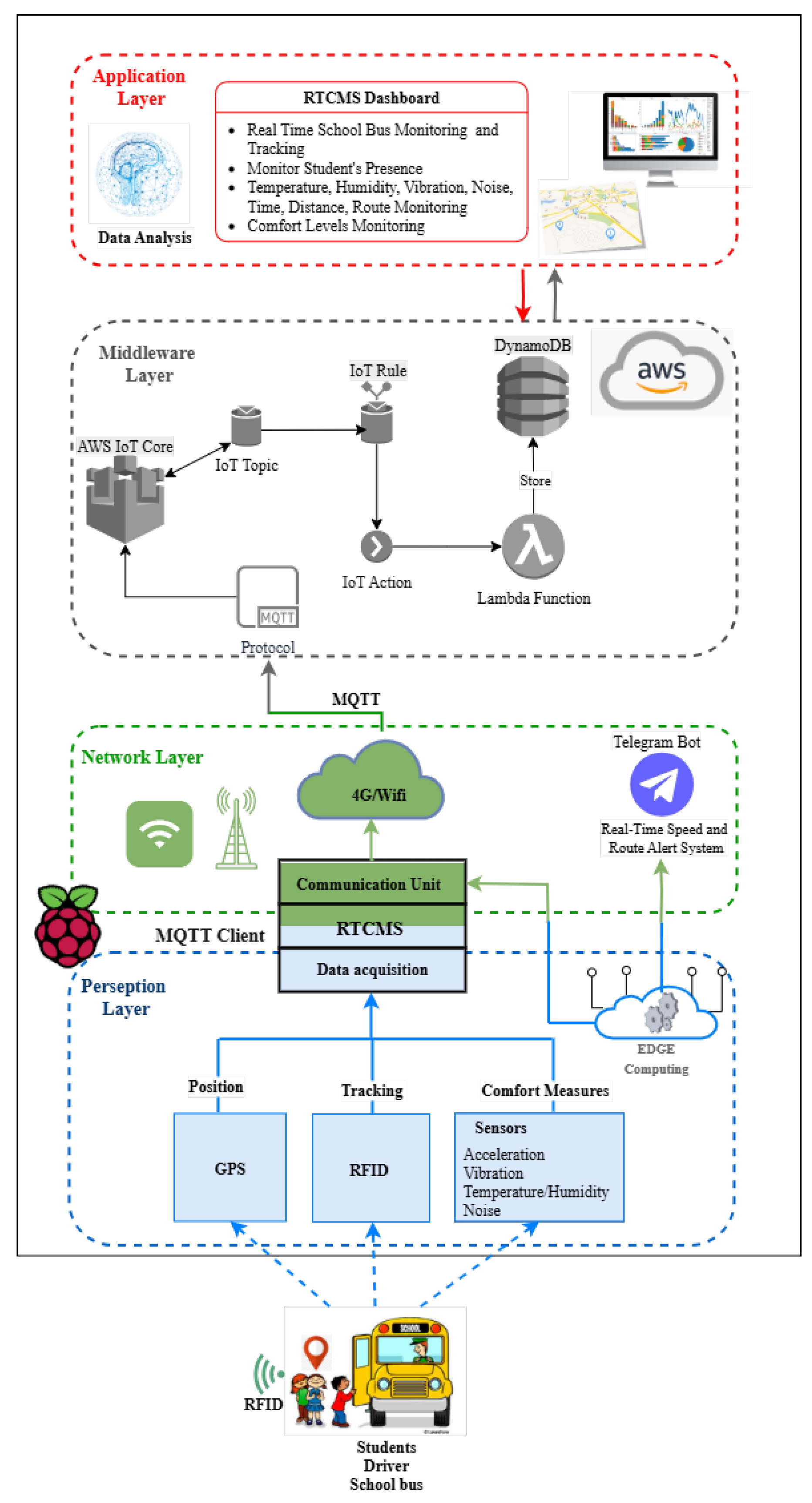
The algorithms used to estimate the comfort score are detailed, along with the sensor fusion strategy implemented in the SBC Figure 2 illustrates the overall architecture of the system, highlighting its four-layer structure.

3.1. Vehicle Platforms Used for Testing

Real-time testing was performed using two types of school vans to ensure variability in vehicle structure and mechanical response. The primary test platform was a Toyota Hiace van, model year 2002, in which most of the initial data acquisition and algorithm validation was performed. To confirm the generalizability of the results and validate the performance of the system under different conditions, the final tests were replicated in a Foton school van, model year 2020. These tests incorporated sensor measurements for temperature, acoustic noise levels, and vibration-induced comfort, consistent with the evaluation framework described in Section 3.2, Section 3.3 and Section 3.4. This dual platform approach ensured a more robust assessment of comfort metrics in diverse mechanical and acoustic environments.

The tests were conducted in the city of Loja, located in the southern region of Ecuador, South America. Loja is a mid-sized city with an estimated population of 200,000 inhabitants [44], known for its relatively well-developed infrastructure and adherence to urban planning standards. However, due to recent climatic variability, certain suburban areas exhibited deteriorated pavement conditions, characterized by increased surface roughness, providing an ideal scenario for test drives under varied conditions.

The final real-time testing phase spanned six days, with each session lasting approximately two hours. Additional runs were conducted to collect data under various conditions on the road surface for use in supervised machine learning training. Due to the demanding nature of driving on rough terrain, only a professional driver and laboratory staff participated in these experiments.

To determine the route paths, a realistic emulation of vehicle trajectories was performed, simulating trips from an educational center to several homes distributed throughout various city sectors and vice versa. The objective was to log the routes, evaluate the comfort scores in multiple parameters, record travel times, and assess the vehicle velocity along each route. Six homes were designated as student pickup points, each equipped with an RFID system for identification. The speed of the vehicle was continuously monitored to detect instances of overspeeding. Although there is no universally accepted standard for the speed of school transport, Braz et al. [45] reports an average operational speed of 32 km/h. In contrast, Ecuadorian legislation [46] specifies that public transport in urban areas should adhere to speed limits ranging from 40 to 50 km/h, and up to 60 km/h in peripheral zones. Importantly, in school zones, the limit is reduced to 20 km/h. Consequently, the system was configured to trigger alert notifications via a Telegram application whenever the vehicle exceeded the 50 km/h threshold during testing.

The RFID-based student tracking subsystem was designed in accordance with the data protection principles of the General Data Protection Regulation (GDPR) [47] and the Organic Law of Ecuador on Personal Data Protection [48]. As this study was conducted in a simulated environment, no real students participated; all identifiers (names, RFID tag IDs) are entirely fictional and are used only for route emulation.

In line with the principle of data minimization, the proposed operational design collects only pseudonymized tag IDs and timestamps, with any mapping to real identities stored in a separate, access-controlled registry. The IoT node does not process personally identifiable information. The planned security provisions include end-to-end encryption: TLS/HTTPS in transit and AES-256 at rest, with access restricted to authorized personnel.

For future real-world deployments, the platform will include explicit informed consent procedures for legal guardians and conduct a Data Protection Impact Assessment (DPIA) to assess privacy risks. These measures will ensure full compliance with GDPR, national legislation, and IoT privacy-by-design best practices.

3.2. Thermal Comfort Assessment

This subsection describes the methodology used to quantify thermal comfort based on real-time ambient temperature measurements collected during transportation. The comfort score reflects deviations from a predefined optimal range, as established by recognized thermal comfort models.

To evaluate thermal comfort within the IoT-based monitoring system installed in the transport unit, temperature (in °C) and relative humidity ($HR$) data were collected using a DHT22 sensor connected to the SBC. Based on these measurements, two complementary assessment approaches were implemented.

The first approach uses the apparent temperature index (ATI), which combines air temperature and relative humidity to estimate perceived thermal conditions. The thermal comfort levels were then derived using Likert scale evaluations, as proposed by Davydova et al. [29].

The second approach relies exclusively on ambient temperature data. Following the classification framework by Lin et al. [25], discrete thermal comfort levels were defined using temperature thresholds. This dual-method strategy provides a more robust assessment of thermal conditions during transport.

The local climate context plays an important role in the interpretation of ATI values. According to Köppen’s classification, Loja city generally falls under the Cfb category [49], depending on elevation and rainfall patterns. This denotes a temperate oceanic climate with no dry season and moderate temperatures during the wet period. Real-time tests were carried out in May and June, which correspond to the end of the wet season and are typically characterized by light drizzle and elevated humidity.

To evaluate thermal comfort in a closed environment, we applied a simplified empirical formula for the Apparent Temperature Index (ATI), which combines air temperature (T, in °C) and relative humidity ($HR$, in %) as follows:

$$\mathrm{ATI}=-63.244+2.526T+0.351HR$$

(1)

This formula was validated with a determination coefficient $R^2=0.9603$, indicating a strong correlation with the perceived thermal comfort data reported in [29].

To better represent thermal perception in highland climates such as the city of Loja, the traditional classification was extended to include a cold stress category, as summarized in

Table 1. Extended thermal comfort classification using ATI.

Category	ATI Range (°C)	Description
Cold Stress	<20	Discomfort due to low temperature
Comfortable	20–28	Ideal thermal range
Moderate Heat	28–33	Mild heat stress, increasing discomfort
Severe Heat Stress	>33	High discomfort, heat stroke risk

.

These thresholds are adapted from the classification defined by the Spanish State Meteorological Agency (AEMET) and further validated by studies conducted in tropical transit environments [29,50].

In addition, to implement a discrete classification system for thermal comfort based solely on air temperature, a set of thresholds was established and is presented in

Table 2. Discrete levels for thermal comfort classification based on air temperature.

Category	Temperature (°C)	Description
Comfortable	21–27	Ideal temperature range for short-haul vehicles
Moderate	28–32	Suboptimal, but tolerable for short-haul conditions
Uncomfortable	<21 or >32	Uncomfortable due to cold or excessive heat

. These values were adapted from the framework proposed by Lin et al. [25], with modifications introduced to reflect the specific conditions of the highland terrain where the study was carried out.

For this part of the analysis, only temperature measurements, collected at 10 s intervals, were used. Comfort levels were designed to represent subjective thermal perception in short-haul transport vehicles, based on empirical observations and previous [25,26,29].

3.3. Acoustic Noise Assessment

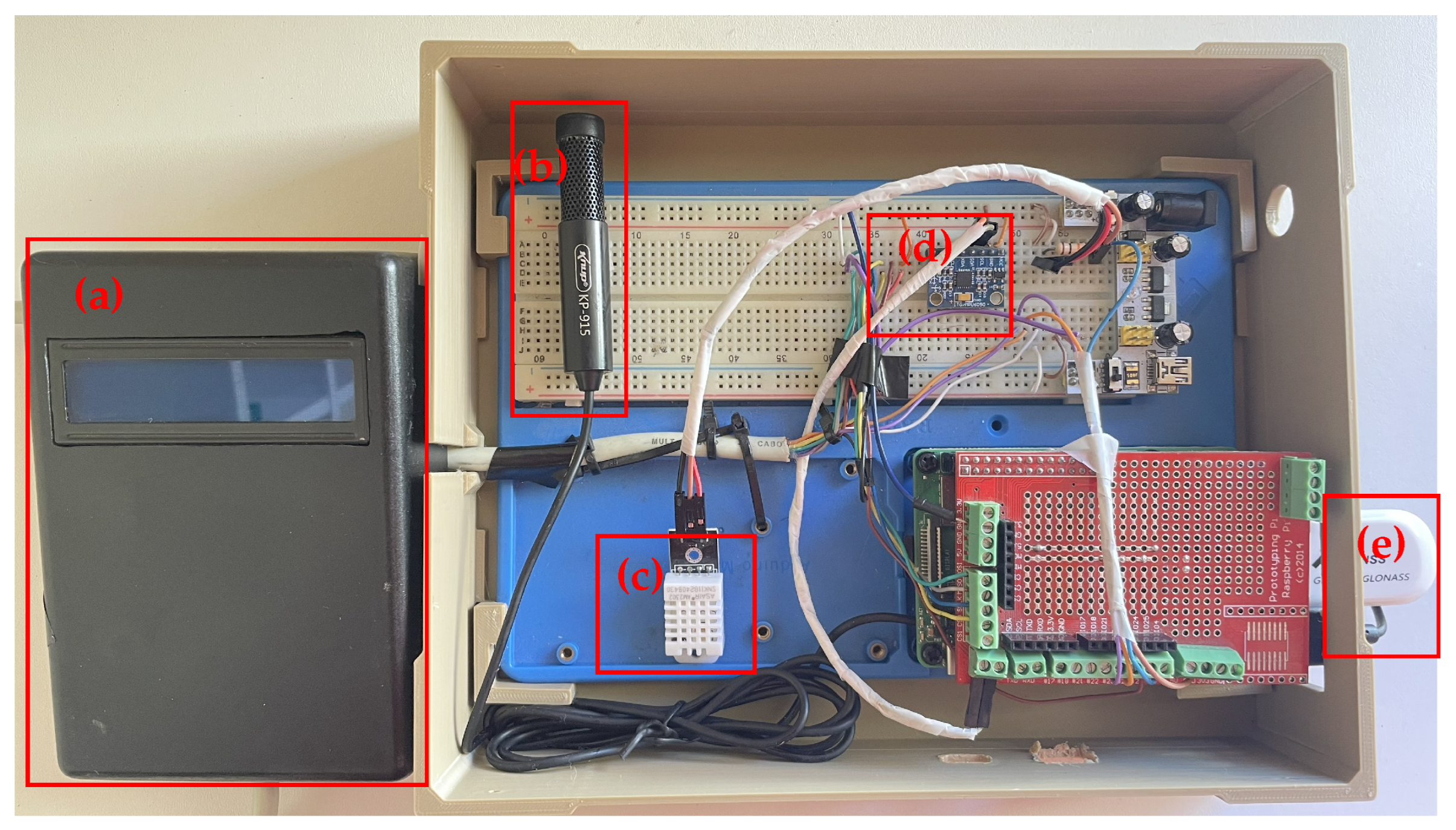
During the real-time testing phase, acoustic data was collected using a Knup KP-915 USB condenser (Knup, São Paulo, Brazil; manufactured in China) microphone connected to the SBC. A custom software-based decibel meter module was developed to measure and record ambient noise levels at 10 s intervals. To ensure consistency and accuracy of the measurement, the system was calibrated against a digital sound level meter, maintaining a linear deviation within ±3 dB(A).

In line with established ergonomic and occupational standards, three discrete acoustic comfort categories were defined for classification purposes:

• Comfortable: ≤65 dB(A)—consistent with NR-17 acoustic comfort guidelines [30].
• Moderate: 66 dB(A) to 80 dB(A)—does not exceed the limits of occupational exposure but may induce discomfort over time [51].
• Uncomfortable: >80 dB(A)—above ergonomic and WHO community comfort thresholds; may pose health risks [34].

To evaluate the responsiveness of the monitoring system and simulate a range of real-world conditions, we introduced controlled acoustic variations inside the vehicle. This was achieved by using the vehicle’s onboard radio as an artificial noise source. The radio volume was adjusted at specific time intervals to simulate realistic scenarios such as background music, noisy conversations, or sudden spikes in ambient noise. These tests were conducted during actual school transport simulation routes, allowing a representative collection of environmental data.

All acoustic data were recorded by the onboard application, which simultaneously provided real-time visual feedback. The collected data set was subsequently used for post-processing and temporal analysis to evaluate the accuracy of the developed decibel meter. The results of this analysis are presented in Section 4, including time series plots that illustrate dynamic noise profiles in different scenarios.

3.4. Standardized Vibration Comfort Assessment

The evaluation of the vibration comfort score index follows the guidelines established in ISO 2631-1 [52], which uses the root mean square (RMS) value of the weighted acceleration signal across three axes. This subsection describes the processes of data acquisition, signal conditioning, filtering, frequency weighting, and computation of the comfort score. The resulting score reflects the perceived quality of the ride and the comfort of the passengers associated with total body vibration.

The SBC interfaced with an MPU6050 inertial measurement unit (IMU) using the I²C communication protocol. The sensor provides raw acceleration data along three orthogonal axes (x, y, and z) with 16-bit resolution and a configurable measurement range of $\pm 2g$. The sensor was mounted on the lower part of the driver’s seat backrest, following the recommendations in [15,36]. To ensure data integrity, the sensor enclosure was positioned away from the gearbox so that the measurements predominantly captured road-induced vibrations rather than engine-related disturbances. Although sensor location can, in principle, influence measured vibration levels, complementary tests on the passenger seat and rear bench showed a high correlation with driver seat measurements. This confirmed that the selected position is representative for the assessment of whole-body vibrations in the tested van-type vehicle, where the shorter wheelbase and suspension system contribute to a more uniform distribution of vibrations between seats. Furthermore, the range $\pm 2g$ of the MPU6050 is sufficient for road vehicle applications, as typical vibration levels remain well below this threshold.

To align with the standard reference frame, Figure 3 illustrates the ISO 2631-1 reference axes for a seated subject. The three translational accelerations evaluated are as follows:

• $a_x$: front-back (anteroposterior) direction,
• $a_y$: side-to-side (lateral) direction,
• $a_z$: vertical direction aligned with gravity.

These directions are the basis for assessing vibration discomfort, with each axis contributing differently to overall perception according to ISO-defined weighting functions.

Before deploying the vibration scoring algorithm on the SBC, the MPU6050 sensor required calibration to ensure accurate baseline readings: $(a_x=0)$, $(a_y=0)$, and $(a_z=1)$, where the latter corresponds to the normalized gravitational acceleration of $1g$. Calibration was performed using the least squares method, and a linear correction model was applied to the raw sensor data [53].

$$a_c\left(t\right)=a_i\left(t\right)-(m_i{a}_i\left(t\right)+b_i)$$

(2)

where $a_i\left(t\right)$ denotes the raw acceleration signal from the sensor, and $m_i$ and $b_i$ are empirically determined scale and bias coefficients for each axis $i\in \{x,y,z\}$. The term $a_c\left(t\right)$ represents the calibrated acceleration. Rather than applying a direct gain-and-bias transformation, the systematic error was modeled as a linear function of the raw signal and subtracted to obtain the corrected value.

After the calibration process, the triaxial acceleration data are acquired for a duration of T = 10 s. Although Zhao et al. [15] used a shorter 1 s acquisition window, we extended this period to 10 s to capture a more representative segment of the road condition. This longer duration allows for a more reliable comfort assessment and helps avoid saturating the cloud processing system by reducing the frequency of data transmission events.

During this acquisition window, the triaxial acceleration is sampled continuously, and a dynamic sampling frequency $f_s$ is estimated:

$$f_s={\displaystyle \frac{N}{T}}$$

(3)

where N is the number of acquired samples.

Signal conditioning is necessary to isolate meaningful motion signals and to comply with the ISO 2631-1:1997 standards. A two-stage filtering process is applied:

• High-pass filter with a cutoff frequency of 0.5 Hz to eliminate gravity and slow drift:

  $$a_{\mathrm{HP}}\left(t\right)=\mathrm{HPF}(a_c\left(t\right),f_c=0.5\mathrm{Hz})$$
• Low-pass filter with a cutoff of 80 Hz to remove high-frequency noise:

  $$a_{\mathrm{LP}}\left(t\right)=\mathrm{LPF}(a_{\mathrm{HP}}\left(t\right),f_c=80\mathrm{Hz})$$

Zero-phase digital filtering using a second-order Butterworth filter is applied via the filtfilt() function from the SciPy library [54].

After conditioning, the signal is transformed to the frequency domain via the Fast Fourier Transform (FFT) to enable spectral analysis.

$$A\left(f\right)=\mathcal{F}\left\{a_{\mathrm{LP}}\left(t\right)\right\}$$

The frequency weightings $W\left(f\right)$ for each axis are applied according to ISO 2631-1:

$$\begin{array}{cc}\hfill W_z\left(f\right)& =\left\{\begin{array}{cc}0.5\hfill & 0.5\le f\le 2\hfill \\ {\displaystyle \frac{f}{4}}\hfill & 2<f\le 4\hfill \\ 1\hfill & 4<f\le 12.5\hfill \\ {\displaystyle \frac{12.5}{f}}\hfill & 12.5<f\le 80\hfill \end{array}\right.\hfill \end{array}$$

(4)

$$\begin{array}{cc}\hfill W_x\left(f\right)=W_y\left(f\right)& =\left\{\begin{array}{cc}1\hfill & 0.5\le f\le 2\hfill \\ {\displaystyle \frac{1}{f}}\hfill & 2<f\le 80\hfill \end{array}\right.\hfill \end{array}$$

(5)

The RMS calculation and comfort index evaluation proceed by computing the weighted RMS acceleration values for each axis over the valid frequency band.

$$a_{\mathrm{rms},i}=\sqrt{\sum _{k=k_0}^{k_1}{W}_i{\left(f_k\right)}^2{\left|A_i\left(f_k\right)\right|}^2}$$

(6)

where $f_k=k·\Delta f$ are the discrete frequency bins obtained from the FFT, $\Delta f=f_s/N$ is the frequency resolution defined by the sampling frequency $f_s$ and the number of acquired samples N, and $k_0,k_1$ correspond to 0.5 Hz and 80 Hz, respectively. Thus, the discretization is linear and directly determined by the FFT resolution.

Where $W_i\left(f_k\right)$ is the frequency weighting function and $A_i\left(f_k\right)$ is the acceleration spectrum for the axis $i\in \{x,y,z\}$.

The total weighted RMS acceleration is then obtained via vector summation, using ISO-prescribed axis multipliers:

$$a_{\mathrm{rms},\mathrm{total}}=\sqrt{{\left(1.4a_{\mathrm{rms},x}\right)}^2+{\left(1.4a_{\mathrm{rms},y}\right)}^2+a_{\mathrm{rms},z}^2}$$

(7)

The quadratic mapping proposed by Zhao et al. [15] was calibrated against a comfort scale defined on total weighted RMS acceleration intervals ranging from <0.135 m/s² to >2.0 m/s². In our experiments, the MPU6050 MEMS accelerometer (InvenSense, San Jose, CA, USA) was configured with a reduced dynamic range of $\pm 2g$, which increased the resolution in the low acceleration domain relevant for comfort analysis. This configuration enabled the detection of very small vibration levels (e.g., $a_{\mathrm{rms},\mathrm{total}}\approx 0.02$ m/s²) under steady-state or excellent road conditions. Under these conditions, direct application of Zhao’s coefficients occasionally produced scores slightly higher than 10 (e.g., $C\approx 10.46$), exceeding the intended scale of 0–10. To address this, we performed numerical simulations and field validations to recalibrate the coefficients, obtaining the adapted form:

$$C=a_{\mathrm{rms},\mathrm{total}}^2-7a_{\mathrm{rms},\mathrm{total}}+10$$

(8)

This expression retains the quadratic structure of the Zhao et al. [15] model but uses coefficients adapted to our sensor configuration and the vibration range observed in our data set. The modification restricts the comfort score to the [0, 10] interval and is in line with subjective reports of excellent road conditions obtained during field trials.

The score ranges from 0 (extremely uncomfortable) to 10 (high comfort), according to the findings of subjective perception studies and the reference tables proposed by Zhao et al. [15] and Castellanos and Fruett [36].

The entire signal acquisition and processing pipeline runs continuously in a concurrent loop on the Raspberry Pi. Comfort scores are updated every (10 s) and can be displayed in real time or stored for later analysis.

3.5. Machine Learning-Based Road Comfort Classification

In addition to the signal-based comfort score defined by ISO 2631-1, a data-driven classification method was developed to automatically label road segments into discrete comfort levels based on vibration patterns. This approach employs supervised machine learning to categorize signals according to road conditions using characteristics derived from the vertical acceleration component ($a_z$), which has the strongest perceptual impact on seated discomfort [15,40,55].

We adopted a supervised machine learning approach because fixed-threshold methods, such as those based solely on RMS acceleration, can underperform in heterogeneous field conditions where vehicle type, suspension response, and road characteristics vary. A Random Forest model was chosen for its balance of classification accuracy, computational efficiency, and interpretability, making it well-suited for embedded, real-time IoT  applications.

The raw acceleration samples were labeled according to the comfort levels defined in

Table 3. Comfort level classes used for road surface labeling.

Level	Road Surface Description
0	Dirt road, no pavement; very rough and uncomfortable
1	Road with potholes or severely damaged pavement
2	Road with several patches; moderate vibration
3	Mostly smooth road with occasional patches
4	Brand-new or recently resurfaced pavement; very smooth ride

. A total of 135 samples were collected at a controlled driving speed of 20–40 km/h to ensure consistency and minimize variability caused by individual driving styles. Specifically, 27 samples were recorded for each comfort level in different locations to enhance the robustness of the model.

Initially, the classification of the road surface was performed using five discrete comfort levels, as shown in Table 3. However, for real-time applications, we observed that a three-level scheme significantly improved both system performance and classification consistency. Based on statistical similarity and signal characteristics, the original levels were consolidated as follows. Levels 0 and 1 were grouped into uncomfortable, Level 2 remained as moderate, and Levels 3 and 4 were grouped into comfortable.

This reclassification required balancing the data set, as the new uncomfortable class contained 54 samples after merging, while the original moderate class included only 27. To achieve class balance, the moderate class was increased to 54 samples, resulting in a total of 162 labeled segments (54 per class), as shown in

Table 4. Reclassification of road surface comfort levels.

New Class	Original Levels Merged
Uncomfortable	Levels 0–1; severely damaged or unpaved roads
Moderate	Level 2; road with patch repairs covering potholes
Comfortable	Levels 3–4; road with minor patching or in good condition

. As discussed in Section 5, this restructuring led to a relative improvement of 28.6% in classification efficacy and enabled smoother real-time operation.

For the classification of vibration comfort levels, a supervised machine learning approach was implemented using a Random Forest classifier. Each 10 s window of vertical acceleration data was transformed into an 11-dimensional feature vector, capturing time-domain, jerk-based, and frequency-domain characteristics:

• Time-domain features (6): Root mean square (RMS), standard deviation, skewness, peak-to-peak value, total signal energy, and zero-crossing rate. These summarize the magnitude, variability, and dynamic range of the vibration signal. In particular, acceleration variability (STD_acc) and dynamic range (Peak2Peak_acc) are key indicators of road roughness intensity, as higher variability and range typically correspond to more irregular and uncomfortable surfaces.
• Jerk-based features (2): RMS and standard deviation of the jerk signal, defined as the discrete derivative of vertical acceleration:

  $$j\left(t\right)={\displaystyle \frac{d{a}_z\left(t\right)}{dt}}\approx {\displaystyle \frac{a_z\left(t\right)-a_z(t-1)}{\Delta t}},\Delta t={\displaystyle \frac{1}{f_s}}={\displaystyle \frac{1}{240}}\mathrm{s}$$
  Jerk features improve sensitivity to abrupt motion changes, such as bumps or potholes, which may not be reflected in acceleration magnitude alone. This aligns with the SHAP analysis, which identified STD_jerk and RMS_jerk as dominant predictors, indicating that sudden vertical acceleration changes strongly correlate with perceived discomfort, as shown in Section 4.5.
  The sampling frequency $f_s=240\mathrm{Hz}$ was chosen considering the maximum frequency of interest of 80 Hz (ISO 2631-1). Although the Nyquist limit requires at least 160 Hz, in practice, a higher rate is used to reduce aliasing and ensure stability. Field tests with the Raspberry Pi 4B showed that 240 Hz provided accurate and stable data, while higher rates (e.g., 500 Hz or 1 kHz) only increased data size and processing time without improving resolution.
• Frequency-domain features (3): Dominant frequency, total spectral power in the 1–10 Hz band (most relevant for seated whole-body vibration), and spectral entropy.
  The spectral power in the 1–10 Hz range captures energy within the frequency band most associated with human whole-body vibration discomfort, as outlined in ISO 2631-1. Spectral entropy distinguishes between smooth harmonic vibrations (low entropy) and chaotic broadband signals (high entropy), which are often linked to rough or damaged road conditions. These features were computed using Welch’s method for estimating the power spectral density, which provides a low-variance spectral estimate by averaging periodograms over overlapping segments.

A total of 162 labeled samples were evenly distributed across three comfort classes: uncomfortable, moderate, and comfortable. The classifier was trained using a Random Forest with 100 estimators, selected to balance accuracy and efficiency. Default hyperparameters were used, and performance was validated through 5-fold stratified cross-validation, which preserved class balance and mitigated overfitting.

The Random Forest model learned patterns from the feature vectors to separate comfort classes. Each decision tree in the ensemble was trained on a random subset of features and data, and final predictions were obtained through majority voting. This ensemble strategy enhances robustness to noise and improves generalization to unseen road conditions.

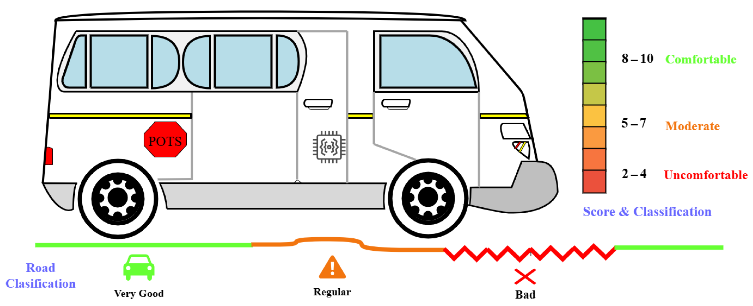
After training, the final model was exported and deployed in the SBC, where it performs real-time classification of the incoming vibration data in 10 s segments. For each window, the classifier outputs one of the three comfort classes. This model enhances on-board analysis by providing discrete and interpretable comfort levels that can be visualized directly or used to trigger alerts. It complements the continuous ISO 2631-1 vibration assessment by enabling rapid decision-making in embedded systems. The model schematic concept is shown in Figure 4.

3.6. Multisensor Rule-Based Comfort Classification

In addition to the machine learning-based vibration classifier, a complementary rule-based algorithm was developed to assess passenger comfort by integrating environmental conditions, such as ambient temperature and noise levels, along with vertical acceleration, to perform a generalized comfort analysis. The system was designed to process real-time signals acquired from embedded hardware installed in the school transport vehicle, operating on 10 s analysis windows at a sampling rate of 240 Hz.

Vertical acceleration data ($a_z$) were segmented into fixed-length windows and processed using the trained vibration classifier described in Section 3.5. In parallel, temperature and noise signals were acquired from onboard sensors and interpolated to match the length of the acceleration signal. For each window, the average temperature and noise levels were calculated and categorized into discrete classes using predefined ergonomic thresholds.

To synchronize the signals from different sensors, linear interpolation was applied to the temperature and noise time series to match the sample length of the acceleration data. Specifically, each environmental signal was resampled to the total number of vertical acceleration samples using NumPy (version 1.23.5) interp() function. This method performs one-dimensional linear interpolation over a uniformly spaced index grid, preserving the overall shape and dynamics of the signal while ensuring alignment with the acceleration data for window-based classification. This step was necessary because environmental signals had a lower or irregular sampling rate compared to the 240 Hz acceleration signal.

Each of the three modalities, vibration, temperature, and noise, produced a discrete class label for each window: 0 for comfortable, 1 for moderate, and 2 for uncomfortable. To integrate these heterogeneous inputs, we employed an adaptation of the Comfort Index (CI) methodology [56]. Specifically, a weighted scoring function S was defined as follows:

$$S=0.6C_v+0.2C_t+0.2C_n$$

(9)

where $C_v$, $C_t$, and $C_n$ represent the class values assigned to vibration, temperature, and noise, respectively. The weighting scheme was determined through simulation experiments that tested multiple proportional configurations in contrasting operational scenarios. These trials consistently indicated that vibration should have the largest influence on the combined score, as it reflects external factors—such as road surface quality and traffic-induced oscillations—that are less amenable to short-term mitigation through vehicle control. In contrast, thermal and acoustic comfort can be more easily adjusted via onboard systems, so their contribution to the overall comfort score was comparatively reduced. This allocation ensures that the integrated decision logic remains sensitive to vibration-related discomfort while still incorporating complementary environmental cues.

The final comfort label $C_f$ was calculated by rounding S to the nearest integer and constraining it to the range [0, 2]. This fusion logic is defined by the following piecewise function:

$$C_f=\left\{\begin{array}{cc}0,\hfill & \mathrm{if}\mathrm{round}\left(S\right)<1\hfill \\ 1,\hfill & \mathrm{if}\mathrm{round}\left(S\right)=1\hfill \\ 2,\hfill & \mathrm{if}\mathrm{round}\left(S\right)>1\hfill \end{array}\right.$$

(10)

This rule-based fusion method allows real-time signals to be interpreted into three categories of passenger comfort: comfortable (0), moderate (1), and uncomfortable (2). A summary of the classification thresholds is presented in

Table 5. Comfort classification thresholds used in rule-based decision logic.

Parameter	Comfortable	Moderate	Uncomfortable
Temperature (°C)	21–27	28–32	<21 or >32
Noise Level (dBA)	≤65	66–79	≥80
Vibration (Model Output)	0	1	2

.

The comfort classification outputs of the system were plotted over time to visualize the evolution of environmental conditions and the quality of the ride throughout the transit period. This multisensor approach improves situational awareness in school transport monitoring and complements ISO 2631-based vibration assessments by incorporating thermal and acoustic factors that contribute to discomfort from a broader perspective.

3.7. Data Visualization, Monitoring, and Postprocessing Framework

The proposed platform implements a complete IoT system, structured according to a four-layer Service-Oriented Architecture (SoA), as illustrated in Figure 1. Each layer plays a specific role in the end-to-end data pipeline, ranging from sensor acquisition to user-facing applications. This section focuses on the Application Layer, which provides real-time visualization, monitoring, and post-processing functionalities to end users, such as school staff, policy makers, and researchers.

Sensor-generated data are transmitted asynchronously and in real time to the AWS cloud infrastructure using the MQTT protocol. Data flow management is handled through AWS IoT Core, where specific policies and routing rules are defined. These configurations trigger AWS Lambda functions that process incoming data and store the results in a NoSQL DynamoDB database. This cloud integration and event-driven data handling form the backbone of the Application Layer in our IoT system, enabling seamless interaction between the network and end-user services.

To support post-processing and visualization, a custom software system was developed using Python (version 3.9) as the core programming language. This system interfaces with DynamoDB and utilizes Pandas and NumPy for data cleaning, transformation, and statistical analysis. Visualization capabilities are provided through a web application built with Flask for the back end and JavaScript (ECMAScript 2020) for the front end, featuring an interactive dashboard.

The dashboard overview summarizes individual comfort levels derived from temperature, noise, and acceleration data and presents a composite comfort index that integrates all three dimensions. Supplementary metrics such as total travel time and distance covered are also displayed. Two interactive maps visualize the general bus routes during the morning and afternoon periods, accompanied by a table listing the students identified by RFID.

Each student record is associated with individualized route data, including maps for home-to-school and school-to-home trajectories. The system automatically computes the duration and distance of the route, highlighting deviations from predefined thresholds through visual cues, such as color-coded indicators, facilitating the identification of anomalies or potentially undesirable conditions. To align with ergonomic and educational recommendations, the system flags cases in which a single trip exceeds 45 min, following national guidelines for rural school transportation [57]. Although 45 min is considered ideal, a maximum duration of up to one hour is tolerated in the referenced study. These thresholds are also used to identify students exposed to long travel durations, which can negatively impact academic performance [9], and to support the planning of more efficient and equitable school transport routes.

The application is organized into five main sections, four of which correspond to specific data types: temperature/humidity, noise, acceleration, and speed. Each section incorporates interactive charts—such as gauges, histograms, min–max bar plots, boxplots, splines, and pie charts—to provide an intuitive and comprehensive interpretation of the data collected throughout the monitoring period. By integrating these visualization and alerting tools into the IoT architecture, the platform closes the loop between data acquisition, cloud processing, and actionable insights, which is a defining feature of IoT-based monitoring systems.

3.8. Sensor Integration and Circuit Setup Using Raspberry Pi 4

A Raspberry Pi 4 Model B single-board computer (SBC) serves as the central unit for data acquisition, local preprocessing, and communication in the Smart Comfort School Transportation platform. The SBC is housed in a protective enclosure designed to withstand automotive vibrations and protect against environmental exposure (Figure 5).

Integrated sensors measure ambient temperature/humidity, vibration, acoustic noise, and geolocation, while an RFID module (privacy safeguards described in Section 3.1) supports passenger identification. Data are transmitted to the cloud in real time via a 3G/4G modem, with Wi-Fi tethering as a backup option. The system is powered from the vehicle’s 12 V DC outlet, converted to a stable 5 V/3 A supply with overcurrent protection and voltage regulation.

Additional engineering considerations, such as enclosure thermal management, sensor calibration, communication bus integrity, and complete hardware specifications, are provided in Appendix B.

4. Results

This section may be divided into subsections. It should provide a concise and precise description of the experimental results and their interpretation, as well as the experimental conclusions that can be drawn.

4.1. Temperature Signal Analysis and Apparent Temperature Index (ATI)

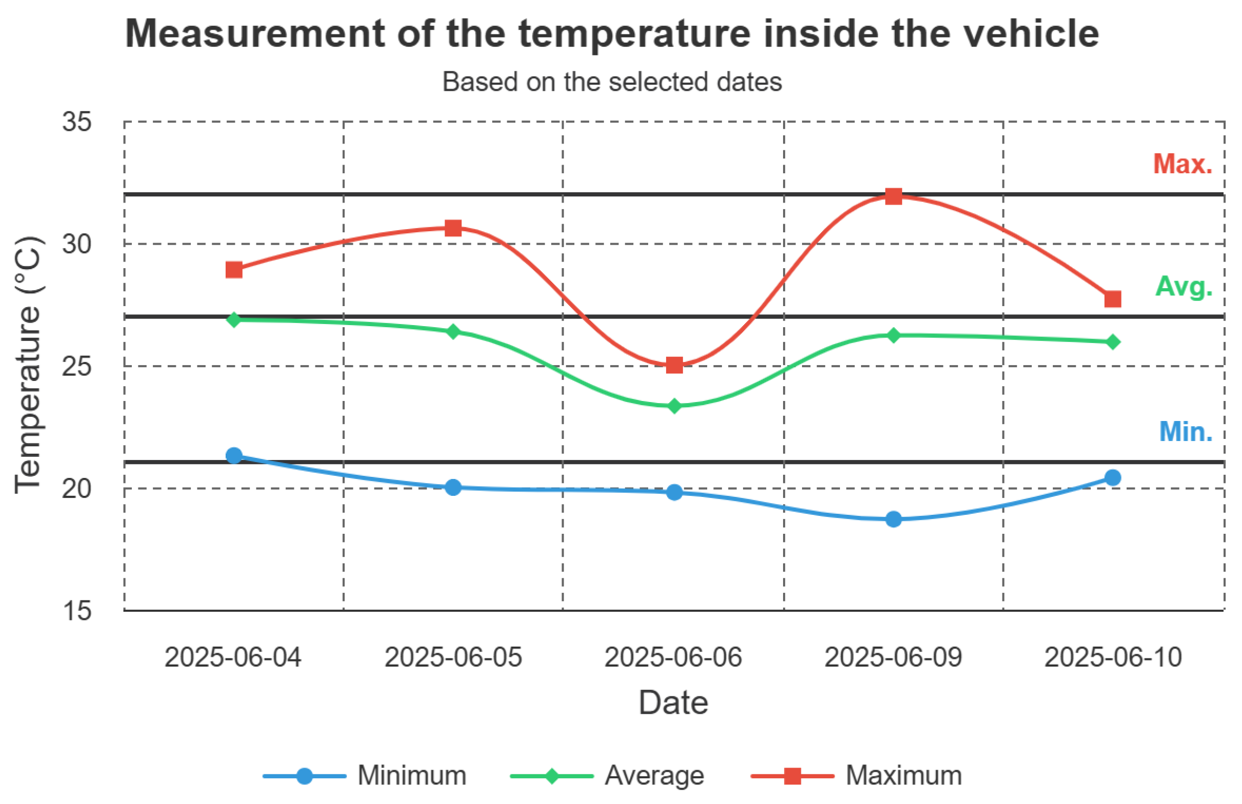
Daily temperature measurements recorded inside the school transport vehicle for five selected days (Figure 6) reveal noticeable variations in the minimum, average, and maximum air temperatures. In this graph only the air temperature was measured; the recorded values can be qualitatively interpreted using the extended thermal comfort classification presented in Table 2. The average daily temperatures generally remained within the “comfortable” range (20 °C to 28 °C), indicating acceptable thermal conditions. However, maximum daily temperatures frequently exceeded 28 °C, entering the category of “moderate heat”, with a peak above 33 °C observed on 9 June, which indicates levels of “severe heat stress”. These findings suggest that, despite moderate average temperatures, short-term exposure to maximum temperatures inside the enclosed vehicle can result in thermal discomfort or heat-related stress, particularly under high humidity conditions or during prolonged exposure. As temperature alone does not fully capture perceived thermal comfort, these results highlight the importance of including additional environmental variables, such as humidity and airflow, in future evaluations. In addition, a time-resolved chart of the evolution of vehicle temperature during daily trips was developed to identify peak temperature events and assess their potential correlation with variations in external ambient temperature.

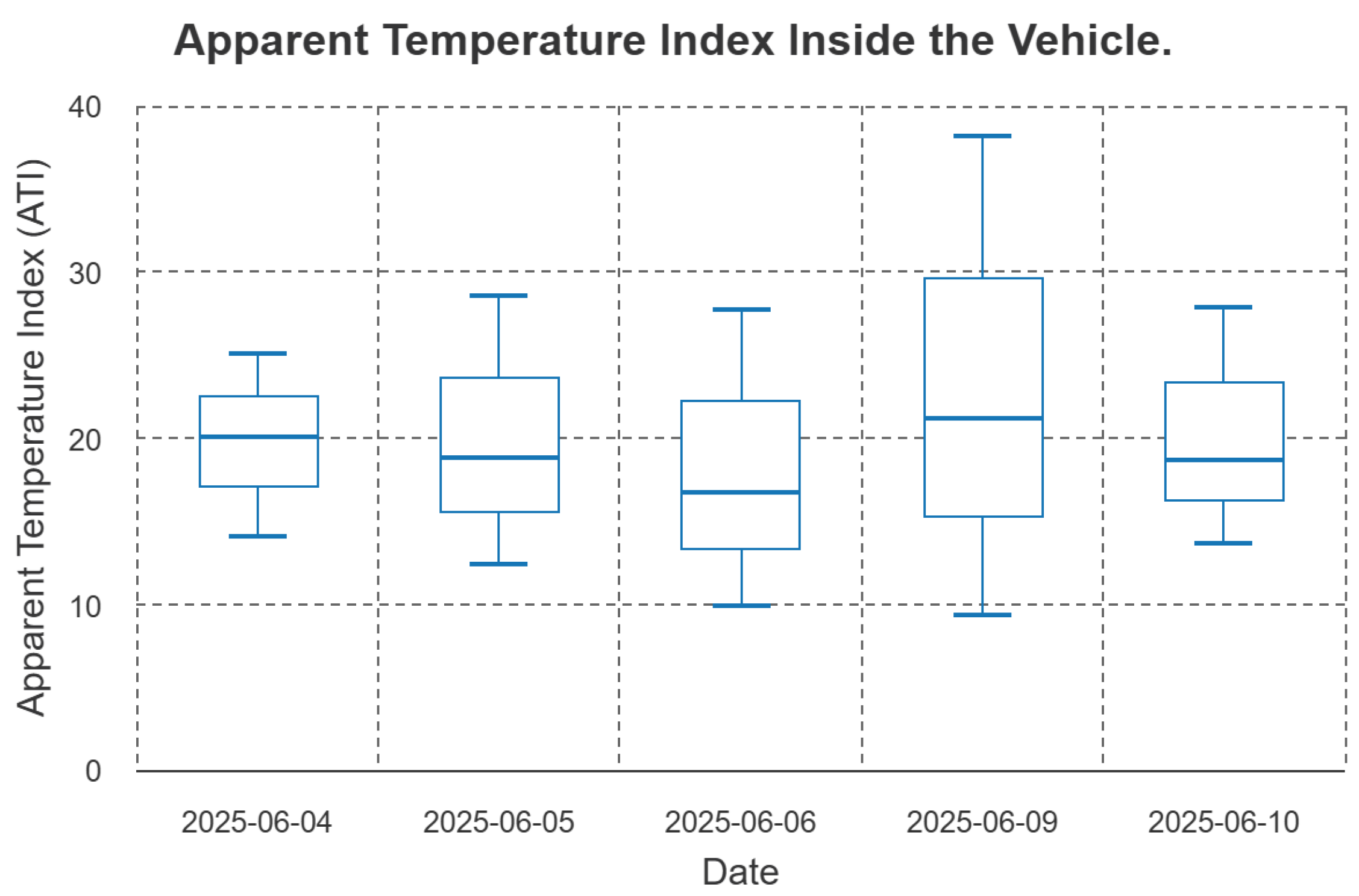
Analysis of temperature, relative humidity, and apparent temperature index (ATI) reveals that ambient temperature alone is not sufficient to accurately assess thermal comfort in school transportation environments. A more comprehensive approach is necessary, one that integrates both temperature and humidity, given their combined influence on human thermal perception. In this context, ATI serves as a composite metric that more effectively reflects actual thermal sensation (Figure 7).

As shown in Figure 7, although the daily maximum temperatures ranged between 25 °C and 32 °C (see also Figure 6), the ATI surpassed 35 °C on several occasions, notably on 9 June. This significant increase in ATI, even on days with moderate average temperatures, is directly associated with elevated levels of relative humidity exceeding 80%. Elevated humidity restricts the body’s ability to dissipate heat through sweat evaporation, thereby amplifying the perceived temperature and reducing overall thermal comfort.

These results highlight the importance of implementing active thermal management strategies within school vehicles. Such measures include improving ventilation, reducing solar heat gain, and incorporating real-time ATI monitoring. One of the simplest and most effective ways to reduce solar heat gain is to park the vehicle in a covered area, such as under a roof or canopy, which significantly lowers interior temperatures by blocking direct sunlight. Together, these interventions can improve thermal comfort and reduce the potential health risks associated with heat stress, especially in school-aged children.

4.2. In-Vehicle Noise Analysis Results

The data visualization of the noise brings a comprehensive overview of noise levels inside the school bus, highlighting both daily trends and intraday variations. Based on the results, the following key observations were identified:

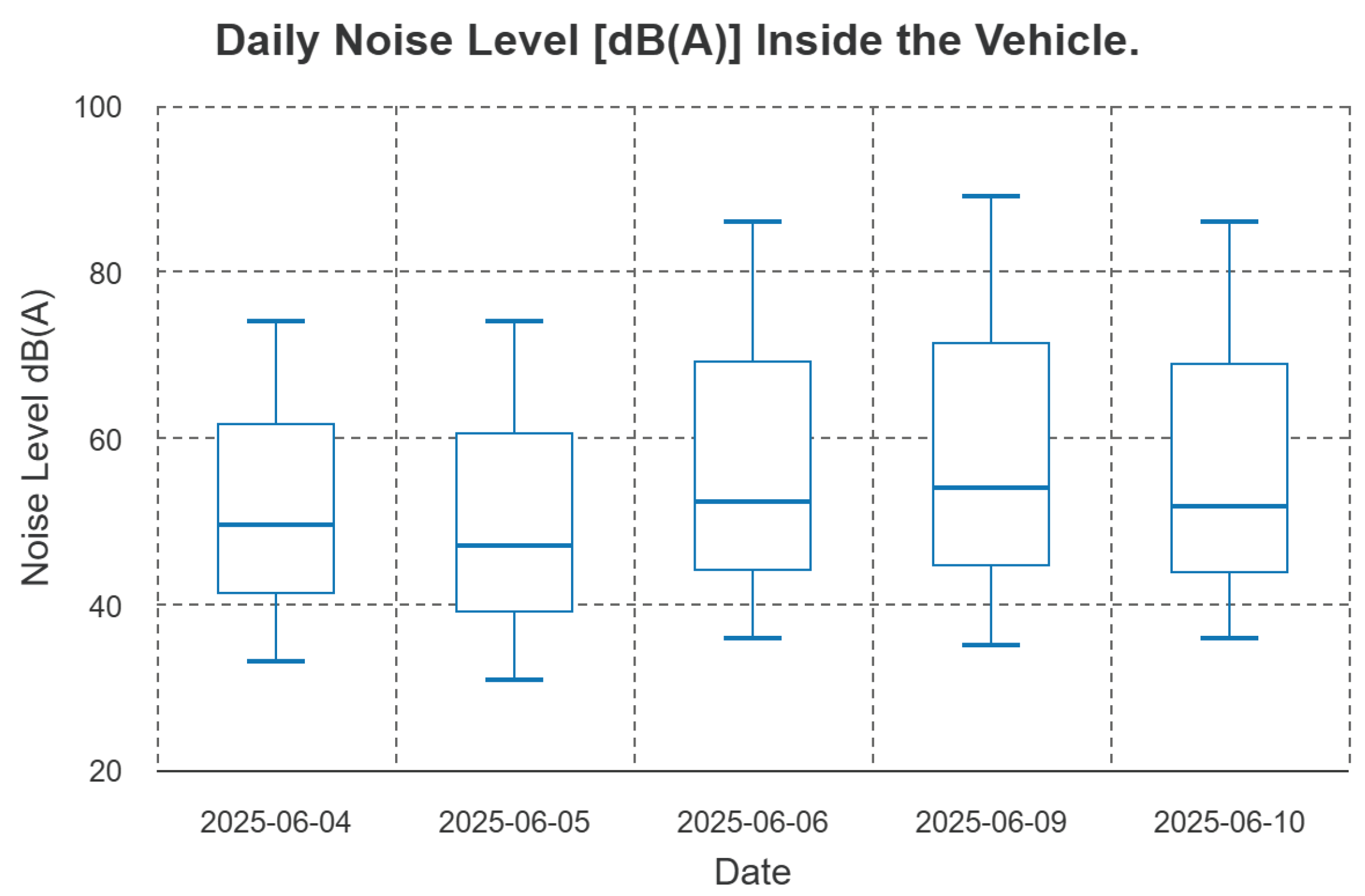
In Figure 8, noise levels exhibit significant variability throughout the day, with median values generally ranging between 45 and 55 dB(A). However, on specific dates such as 6, 9, and 10 June, greater dispersion and peak levels were observed that exceeded 85 dB (A), indicating acoustically unstable conditions. These peaks were mainly caused by increased radio volume, as described in Section 3.3.

Figure 9 presents the fluctuation of sound levels within a selected time window during the day, showing a relatively consistent pattern in which the noise levels varied between 45 and 70 dB(A). However, short-duration peaks were detected above 80 dB(A), particularly in the afternoon period. According to the driver’s experience, noise levels tend to be lower in the mornings, especially because students are typically sleepy. In contrast, during the afternoon return trip, noise levels increase, which is considered normal under such conditions.

4.3. Vehicle Speed Analysis

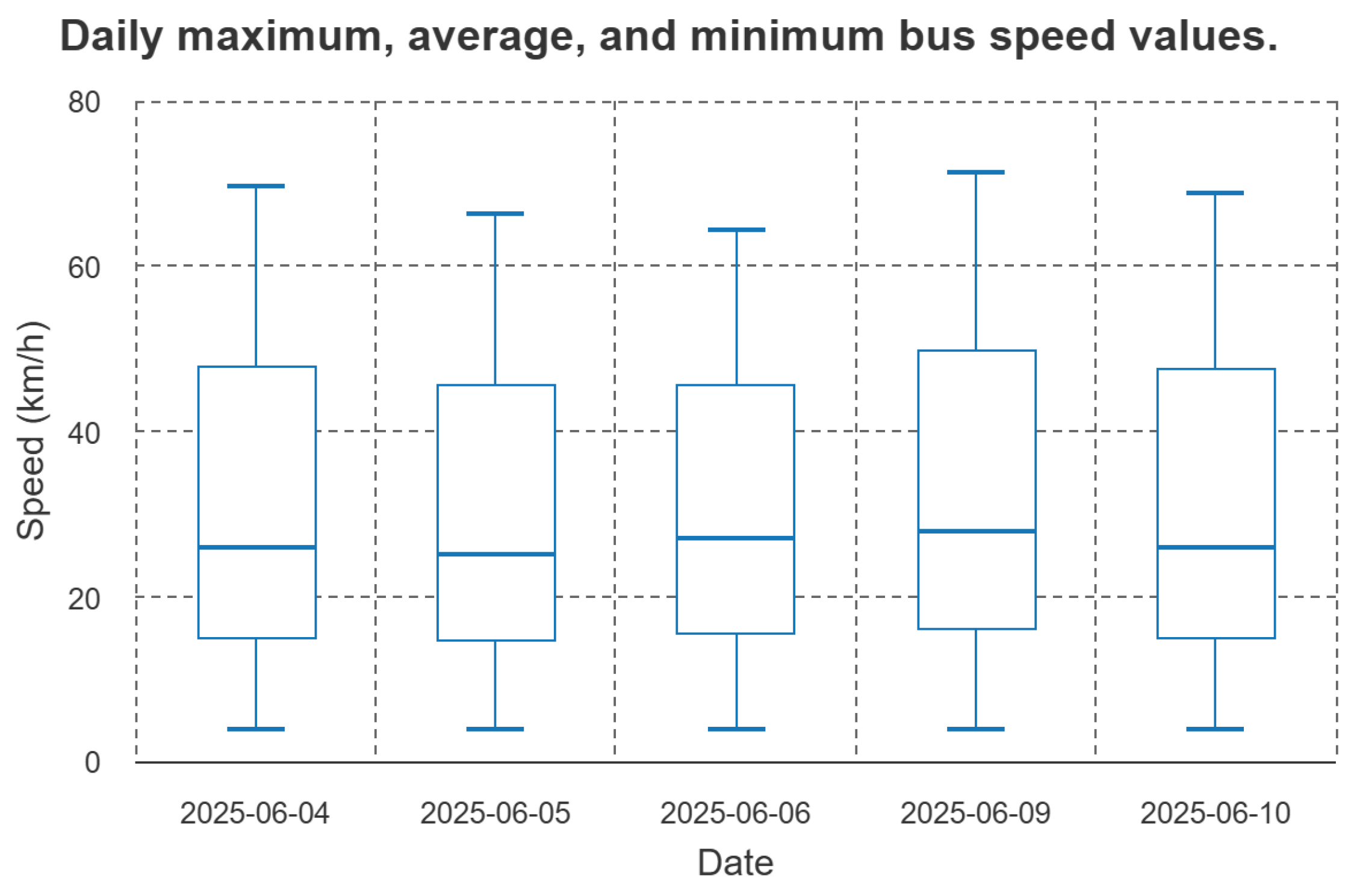
Figure 10 presents the daily statistical distribution of the speed of the school vehicle over a selected period, using box plots to represent the minimum, maximum, and median values. Minimum speeds, typically ranging from 5 to 10 km/h, probably correspond to stops at traffic lights, student pick-up/drop-off zones, or congested segments. In contrast, maximum speeds varied between 65 and 70 km/h, suggesting segments along highways or peripheral roads.

It is important to note that these data were collected during controlled test runs, without students on board. Only the professional driver and the operational laboratory staff were present to ensure safety. In certain peripheral areas, deliberate overspeeding was authorized in order to test system behavior, capture critical data samples, and validate the activation of alerts via the Telegram application.

During the five days, excessive speed was observed, exceeding the recommended limits for school transportation. The median speed consistently fell between 25 and 30 km/h, indicating steady operation under moderate urban traffic conditions. The homogeneity of the data suggests stable driving behavior and route conditions, with no major anomalies or erratic speed variations.

Figure 11 illustrates the vehicle’s speed variation throughout a selected day. Most of the route maintains speeds between 25 and 50 km/h (yellow segments), while higher-speed segments (above 50 km/h, marked in orange) and occasional peaks exceeding 60 km/h (red) are also evident. Lower-speed segments (blue and green) reflect stop phases, slow traffic, or acceleration zones of vehicles, typical of urban environments or school boarding areas.

4.4. Assessment of Whole-Body Vibration Using RMS Acceleration (ISO 2631-1)

Before hardware deployment, the ISO 2631-1 comfort score computation was validated using synthetic triaxial acceleration signals. Several simulated vibration profiles were evaluated to examine the algorithm response under different operating conditions. For clarity, here are two representative cases to illustrate the contrast between extreme scenarios: a low-noise profile (comfortable) and a high-noise profile (uncomfortable). These tests confirmed the sensitivity of the comfort score to vibrational disturbances and verified the correct implementation of the preprocessing and weighting steps in the evaluation pipeline, as illustrated in

Table 6. Comparison of comfort score results and RMS acceleration values under simulated low-noise (comfortable) and high-noise (uncomfortable) conditions, ISO 2631-1 standard.

Parameter	Low-Noise/Not Unomfortable	High-Noise/ Uncomfortable
Weighted RMS X (G)	0.0388	0.1678
Weighted RMS Y (G)	0.0350	0.1691
Weighted RMS Z (G)	0.0779	0.3861
Total Weighted RMS Acceleration (G)	0.1069	0.5101
Comfort Score (Raw)	9.91	7.51

.

The classification of the raw comfort scores follows Zhao et al. [15], in which participants associated discrete numerical values with subjective perceptions of discomfort (10 = “Not uncomfortable,” 8 = “Little uncomfortable,” 6 = “Uncomfortable,” 4 = “More uncomfortable,” 2 = “Very uncomfortable,” 0 = “Extremely uncomfortable”). Since intermediate values are not explicitly defined in that scale, they can be interpreted as lying between two adjacent categories. In this context, the score of 7.51 obtained for the high-noise profile lies between “Little uncomfortable” and “Uncomfortable.” We classified it as “Uncomfortable” to emphasize its deviation from the comfortable range and its proximity to the lower category.

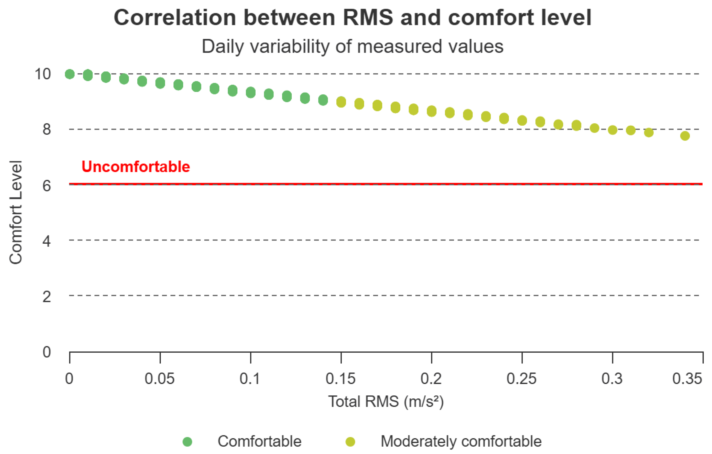
Figure 12 illustrates the correlation between the total weighted Root Mean Square (RMS) acceleration and the corresponding comfort level, as defined by the ISO 2631-1 standard, using real signals acquired from the MPU6050 sensor. The horizontal axis represents the total weighted RMS acceleration (in m/s²), while the vertical axis denotes the computed comfort level on a scale from 0 to 10. The observed data clearly demonstrate an inverse relationship: lower RMS values (e.g., 0.05 m/s²) correspond to higher comfort levels (around 10), whereas higher RMS values (e.g., 0.30 m/s²) are associated with reduced comfort levels (around 8). The gently curved trend follows the quadratic relationship prescribed by the ISO standard, confirming the non-linear dependence between vibration intensity and perceived comfort.

Figure 13 presents a heat map of the comfort levels estimated from the acceleration of RMS on the day of 10 June 2025. The horizontal axis represents the time of day in hourly intervals, while the color scale reflects comfort levels ranging from 0 (very uncomfortable) to 10 (highly comfortable). The predominance of green tones indicates that most of the transport period maintained comfort levels above 9. Only a few isolated segments briefly dropped into the 6–8 range, indicating momentary exposure to discomfort, likely caused by sudden road irregularities or maneuvering. The comfort mapping of the urban area of Loja, based on the RMS acceleration model in accordance with ISO 2631-1, is presented in Appendix A.

4.5. Vibration Classification Performance via Machine Learning

To evaluate the performance of vibration comfort classification using five discrete classes (levels 0–4), a Random Forest classifier was trained on 135 labeled samples, with 27 instances per class. Each input vector contained three time-domain features (RMS, standard deviation, and skewness) extracted from 10 s vertical acceleration windows.

A 5-fold stratified cross-validation procedure was employed to assess the generalizability of the model while maintaining balanced class distributions across folds. The resulting confusion matrix is shown in Figure 14, which illustrates the distribution of true versus predicted labels.

The classification performance across the five folds is summarized in

Table 7. Cross-validation results for 5-class comfort model.

Fold	Accuracy
1	0.7407
2	0.5926
3	0.7407
4	0.7037
5	0.7037
Mean Accuracy	$0.70\pm 0.05$

. The mean accuracy was 70% with a standard deviation of $\pm 5\%$, indicating reasonable performance for fine-grained classification based on a minimal set of characteristics.

The highest accuracy was observed for the central class (Level 2), while some confusion was present between adjacent classes, such as Levels 0–1 and 3–4. These overlaps are expected due to the gradual nature of road surface transitions and driver perception variability. Despite the compact feature set, the model provided a satisfactory balance between granularity and robustness, suitable for embedded system deployment.

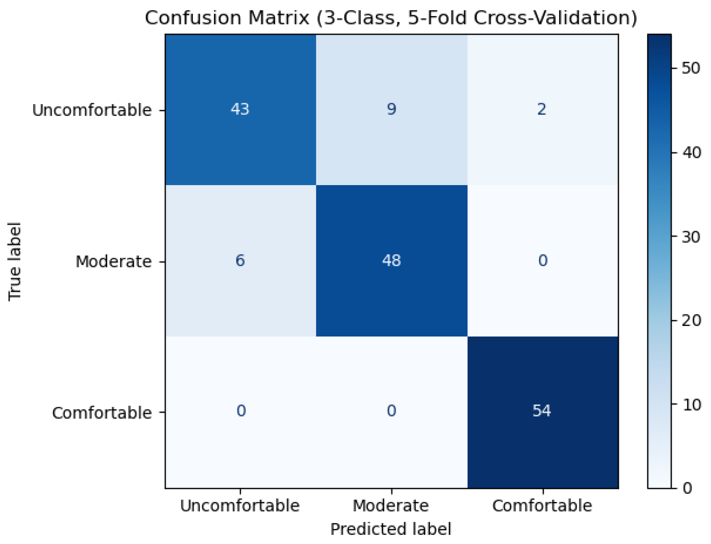
To simplify deployment in real-time conditions and improve classification robustness, the original five-level comfort scale was reduced to three aggregated classes: uncomfortable (merged levels 0 and 1), moderate (level 2), and comfortable (merged levels 3 and 4). The data set was balanced to include 54 samples per class, resulting in a total of 162 labeled windows.

The confusion matrix in Figure 15 shows a strong classification performance across all comfort levels. The comfortable class achieved a level of perfect accuracy. Most of the classification errors occurred between the neighboring uncomfortable and moderate classes, likely due to gradual transitions in vibration patterns.

The accuracy values obtained for each fold, along with the overall mean accuracy, are summarized in

Table 8. Stratified 5-fold cross-validation accuracy results for the 3-class model.

Fold	Accuracy
Fold 1	84.85%
Fold 2	90.91%
Fold 3	90.63%
Fold 4	93.75%
Fold 5	87.50%
Mean Accuracy	90.00% ± 3.00%

. The classifier achieved a mean accuracy of 90% with a standard deviation of $\pm 3\%$, indicating good generalizability.

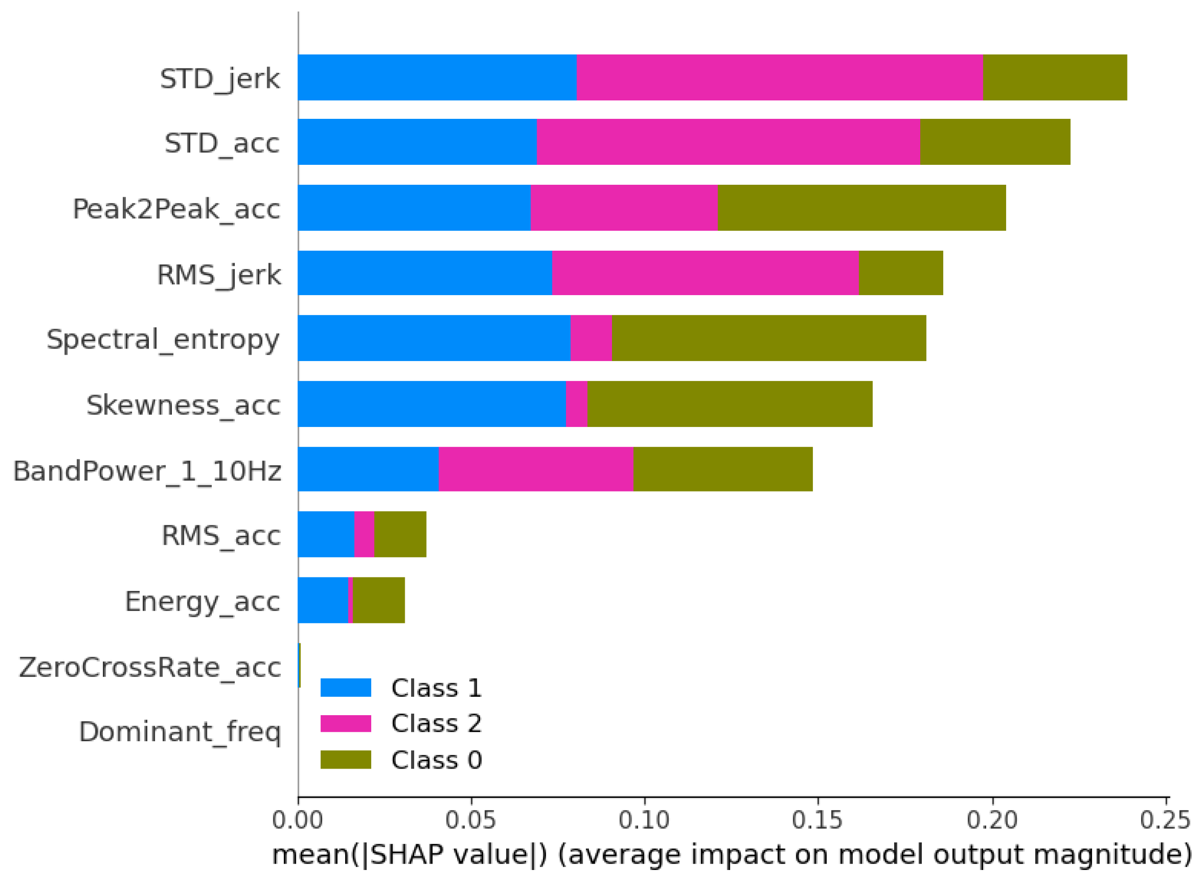
To improve the interpretability of the model, SHAP analysis (SHapley Additive exPlanations) was applied to quantify the contribution of each feature to the classification. Figure 16 shows that the most influential predictors were the standard deviation of jerk (STD_jerk), standard deviation of acceleration (STD_acc), and peak-to-peak acceleration (Peak2Peak_acc), followed by RMS jerk and spectral entropy. These features are consistent with the physics of road-induced vibration, where sudden vertical acceleration changes and higher variability are associated with lower comfort levels. Spectral entropy further differentiated smooth, low-discomfort profiles from irregular, high-discomfort vibrations.

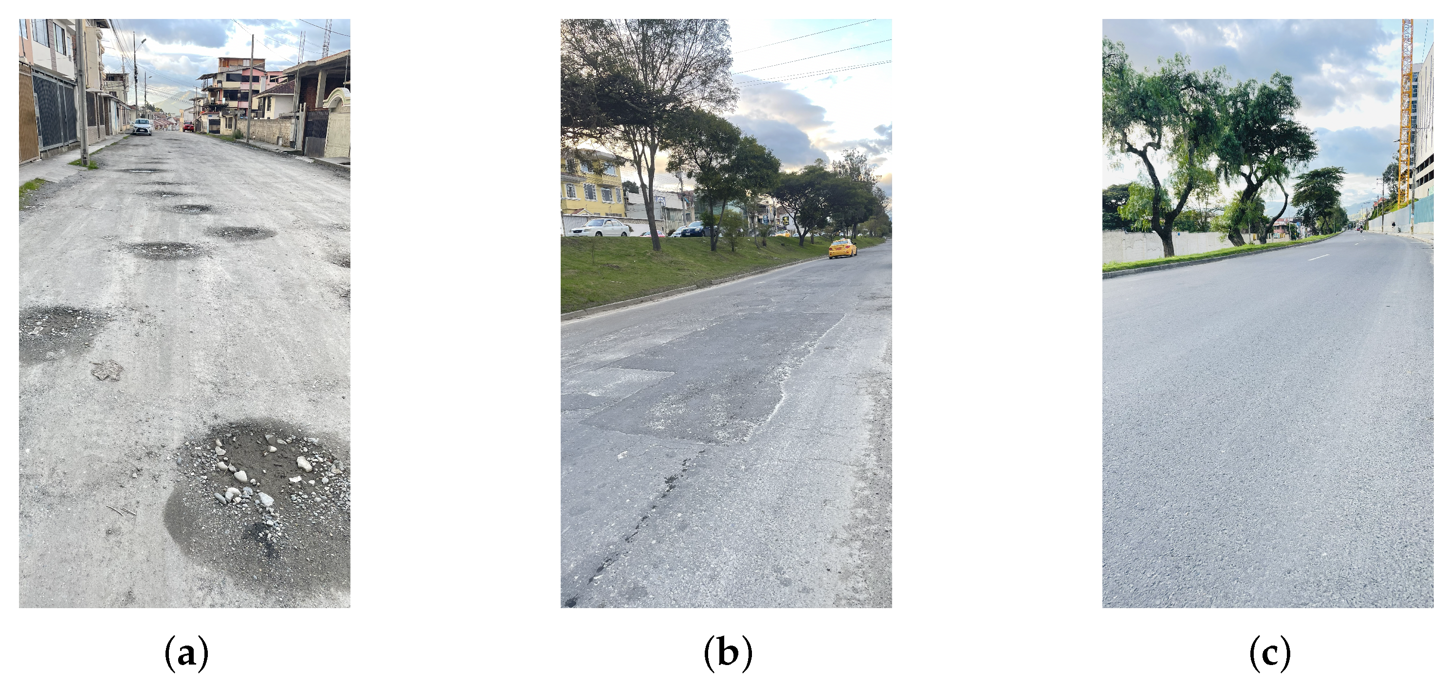
Figure 17 shows representative road segments in the city of Loja where data was collected for vertical vibration analysis using the Random Forest classifier. Sampling was conducted under various road conditions to improve the robustness of the classification system, with labels assigned over 10 s analysis windows. In general, the segments labeled as uncomfortable correspond to unpaved roads or areas with severe potholes. The moderate class typically includes roads with patches or partial surface degradation. Finally, the segments labeled as comfortable refer to well-maintained or recently paved roads.

To assess the robustness and generalization ability of different comfort estimation methods, we compared a rule-based vibration classification using RMS with the ISO 2632-1 standard with a supervised machine learning (ML) classifier trained on data from a different vehicle. The RMS method was applied to a 2020 Foton Scholar van over a segment of a 30 min urban route in the city center of Loja, while the ML classifier was tested on another segment of the same route.

Despite differences in suspension characteristics and segment-specific road conditions, both methods produced consistent results. The RMS-based analysis classified over 92% of the samples as comfortable or very comfortable, while the ML classifier yielded 86.7% comfortable and 13.3% moderate.

These results indicate that the ML model, trained on a 2002 Toyota Hiace van, was well generalized to a different vehicle platform. This has practical relevance for heterogeneous school transport fleets, where uniform calibration across vehicle types is challenging.

Table 9. Comparison of comfort classifications from RMS thresholds and ML classifier.

Method	Comfortable (%)	Moderate (%)	Uncomfortable (%)
RMS Threshold-Based	92.0	8.0	0.0
ML Classifier	86.7	13.3	0.0

summarizes the classification distributions for both methods.

4.6. Results of the Multisensor Rule-Based Comfort Classification

An of the main objectives of this study was to assess the generalizability of the proposed comfort assessment framework in real world conditions. To this end, we applied the multisensor rule-based classification scheme, which combines machine learning-based vibration analysis with threshold-based evaluations of temperature and noise, to data from an actual school transport route. This method is designed to complement both the ISO 2631 reference evaluation (Section 3.4) and the single-modality vibration classification (Section 3.5), providing a unified comfort label suitable for operational deployment.

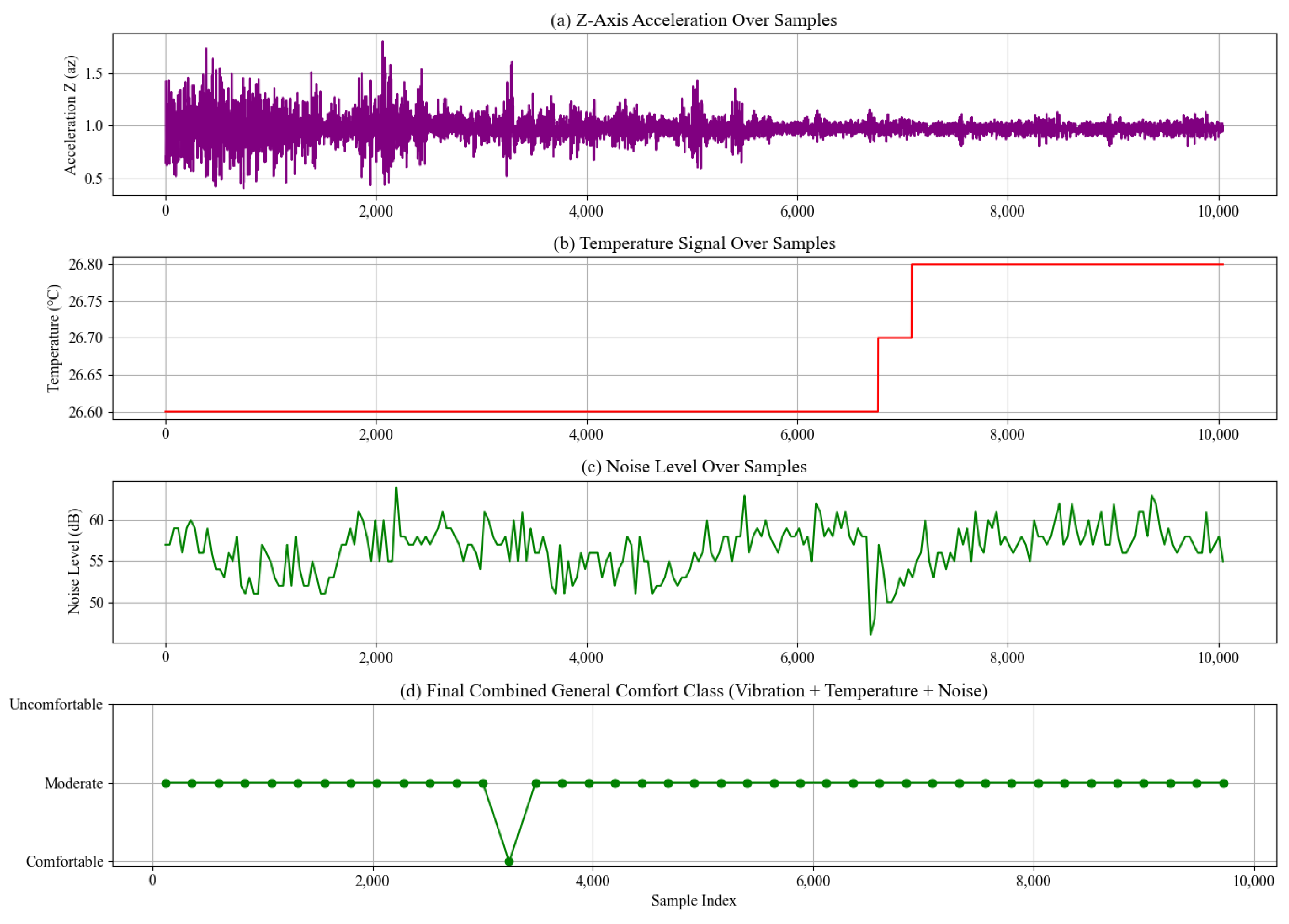
Figure 18 presents the result of a multisensor rule-based comfort classification applied to real-world data collected along a school transport route. The first panel shows the merged vertical acceleration ($a_z$) time series, where fluctuations remain predominantly within moderate vibration magnitudes, with occasional peaks indicative of localized road irregularities. The second panel displays the interpolated temperature profile, which exhibits a stable thermal environment in the range of 26.6–26.8 °C, well within the defined comfort band. The third panel illustrates the noise level signal, characterized by variability between 50–65 dB, remaining under the threshold for moderate classification for the majority of the trip. All signals were linearly interpolated and resampled to ensure temporal alignment with the vibration data, allowing synchronized analysis in fixed-duration windows rather than isolated sensor views.

The bottom panel shows the resulting combined comfort classification derived from the weighted aggregation of the three modalities (vibration: $0.6$, temperature: $0.2$, noise: $0.2$). This rule-based fusion produced a sequence dominated by the moderate class, interspersed with a brief period classified as comfortable. The absence of uncomfortable segments is explained by the combination of vibration levels consistently classified as comfortable or moderate and temperature and noise signals that remain entirely within their respective comfort ranges, preventing the aggregated score from reaching the highest discomfort category. These results demonstrate the ability of the proposed multisensor fusion to integrate heterogeneous measurements into a coherent comfort assessment timeline under operating conditions representative of a well-maintained school transport service.

To quantitatively assess the effect of integrating the auxiliary sensing modalities, we compared the vibration-only baseline against two multimodal fusion strategies: a supervised stacking fusion approach and an entropy-gated fusion scheme. As shown in

Table 10. Overall comfort classification (3 classes). Purged, stratified 5-fold CV. Macro-F1 (mean ± SD) with absolute/relative improvements vs. vibration-only. Wilcoxon signed-rank tests are one-sided for greater performance.

Method	Macro-F1 (Mean ± SD)	$\mathbf{\Delta }$ abs.	$\mathbf{\Delta }$ rel.	p (Wilcoxon)
Vibration-only (no RMS/Jerk)	$0.415\pm 0.099$	—	—	—
Stacking fusion (learned)	$0.476\pm 0.056$	$+0.061$	$+14.7\%$	$0.0448$
Entropy-gated fusion	$0.255\pm 0.088$	$-0.160$	$-38.6\%$	$0.9688$

, the vibration-only model reached a Macro-F1 of $0.415\pm 0.099$, while stacking fusion improved this to $0.476\pm 0.056$, representing an absolute gain of $+0.061$ (≈+14.7% relative), which was statistically significant ($p=0.0448$; one-sided Wilcoxon signed rank test). Entropy-gated fusion, in contrast, performed poorly with a Macro-F1 of $0.255\pm 0.088$ ($-38.6\%$ relative), indicating that in this data set the gating criterion did not effectively exploit auxiliary information.

Table 11. Per-class F1-score (mean ± SD) across folds, with absolute improvements of fusion methods vs. vibration-only.

Class	F1 (Mean ± SD)			$\mathbf{\Delta }$ abs. vs. Vib
	Vib-Only	Stacking	Gated	Stacking	Gated
Comfortable	$0.491\pm 0.180$	$0.535\pm 0.172$	$0.494\pm 0.041$	$+0.044$	$+0.003$
Moderate	$0.324\pm 0.210$	$0.363\pm 0.227$	$0.164\pm 0.225$	$+0.039$	$-0.160$
Uncomfortable	$0.430\pm 0.358$	$0.530\pm 0.287$	$0.107\pm 0.132$	$+0.100$	$-0.323$

breaks down the results by comfort class. Stacking fusion produced consistent improvements across all categories, with gains of $+0.044$ for comfortable, $+0.039$ for moderate, and a substantial gain of $+0.100$ for uncomfortable rides, the latter being the most challenging class. The entropy-gated approach offered negligible benefit for comfortable cases and sharply degraded precision for both moderate ($-0.160$) and uncomfortable ($-0.323$) classes. These results suggest that the learned stacking strategy was better suited to the variability and noise characteristics of the data set, allowing a more robust exploitation of multimodal inputs for comfort classification.

4.7. Route Monitoring and Travel Imbalance Analysis

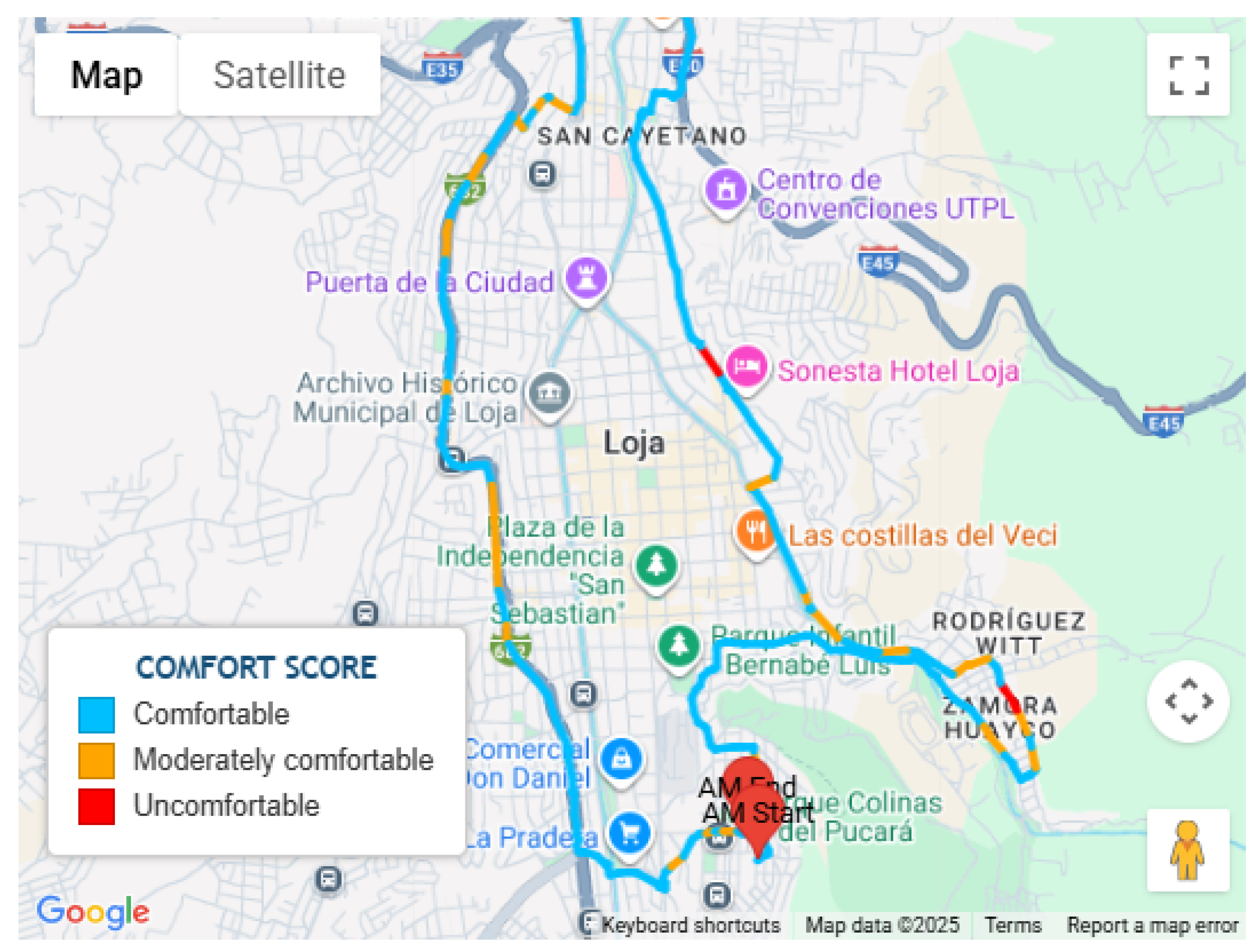
Figure 19 presents the route analysis and travel statistics of a simulated school commute for a monitored student, as visualized on the dashboard interface. A substantial discrepancy is observed between the morning and afternoon trips. The maps show that the morning route covers a significantly longer distance, approximately 17.94 km compared to only 4.5 km in the afternoon. This difference has a direct impact on the duration of the trip. The morning trip lasts 52 min, exceeds the recommended limit, and triggers a red warning indicator. In contrast, the afternoon route is markedly shorter and more efficient, with a duration of only 12 min, well within acceptable limits. This disparity is primarily attributed to the student’s pick-up order in the morning route.

The bar charts on the dashboard reinforce these findings. The distance in the morning remains consistently high on multiple days, around 18 km, while the distance in the afternoon remains low and stable. A similar pattern is seen in travel times: the morning commute consistently takes longer, whereas the afternoon commute is shorter and more predictable.

The mapped route analysis reveals two clearly distinct paths. The morning route is longer and more complex, likely involving detours or multiple pick-up points. In contrast, the afternoon route appears to be more direct and optimized in terms of both distance and time. In particular, certain segments of both routes are highlighted in red, indicating zones where the speed limit for school transportation was exceeded, a safety concern that warrants attention.

These results highlight an operational imbalance between the morning and afternoon commutes, with potential negative consequences for the students’ experience. Extended durations during the morning can contribute to increased fatigue or discomfort, especially when combined with other environmental stressors, such as noise, temperature, and vibration.

This information is essential to inform improvements in school transportation planning. Potential interventions include rerouting, redistribution of student pick-up points, or optimization of the schedule to promote more balanced, comfortable, and safe travel conditions.

A Telegram-based application was developed to send simulated notifications to parents or guardians, providing real-time updates on different aspects of the school journey. The system supports multiple types of notification: start of the trip, safe arrival at school, start of the return trip, and safety alerts. For illustration, Figure 20 presents an example of a safety-related message: a warning issued when the vehicle exceeded the speed limit during a monitored segment. Based on driver feedback, these notifications can improve parental awareness and reassurance by providing timely and relevant travel information.

5. Discussion

This study hypothesizes that a modular, low-cost, and real-time IoT platform that fuses heterogeneous sensor data, such as temperature, noise, and vibration—processed using standardized methods ISO 2631-1 and complemented by machine learning classification—can produce more accurate and context-sensitive comfort assessments than single-sensor or threshold-based approaches. This integrated system will operate reliably under real-world school transport conditions, maintaining data integrity, classification performance, and alert capability even in resource-constrained environments [12].

The cross-vehicle evaluation revised in Section 4.5 demonstrates that the proposed ML approach maintains classification consistency despite differences in suspension systems and route segments. This robustness is particularly important for deployment across mixed fleets, where retraining or per-vehicle calibration may be impractical. The slightly higher sensitivity of the ML classifier compared to the RMS method suggests that it can detect subtle comfort degradations, potentially improving the early detection of maintenance or operational issues. These capabilities were reinforced by previous simulation experiments designed to identify weighting and feature combinations that best preserved classification stability under varying operational profiles.

The comparative evaluation in Section 4.6 confirms that the incorporation of heterogeneous sensor data through a learned stacking fusion approach enhances comfort classification beyond what is achievable with vibration-only models. The improvement was consistent in all comfort categories, with the greatest relative benefit in detecting uncomfortable rides, a critical operational requirement for school transport monitoring. This suggests that even when auxiliary modalities, such as temperature and noise, maintain stable categorical labels, their probabilistic outputs can encode subtle variations that a trainable fusion model can exploit. In contrast, the entropy-gated fusion strategy, which relies on fixed heuristics, failed to capture these nuances and, in some cases, degraded performance. These findings align with previous multimodal learning research showing that adaptive fusion mechanisms are better suited for scenarios where modalities have differing distributions but carry complementary information. Collectively, the results support the central hypothesis: a modular IoT platform that integrates vibration, temperature, and noise through an adaptive fusion layer can deliver more context-aware and operationally relevant comfort assessments than single-modality or rule-based fusion methods.

The evaluation of ATI and the temperature-only classification confirms that the incorporation of humidity in the assessment of thermal comfort substantially changes the operational picture. Although temperature-based thresholds (Table 2) classified most of the monitored trips as within or near the comfort range, ATI revealed multiple episodes of severe heat stress, particularly during high humidity conditions near the end of the wet season. This finding is consistent with the observations of Davydova et al. [29], who reported that elevated humidity levels can significantly increase perceived discomfort in public transport environments, even when measured air temperatures remain within nominal comfort thresholds. Although their study was conducted in the warmer subtropical climate of Guadalajara, Mexico, the underlying mechanism, where humidity amplifies thermal stress, is also relevant in the humid high-altitude conditions of Loja.

From an operational standpoint, this distinction is critical for real-time monitoring in school transport. Temperature-only metrics, as used in earlier public transport comfort studies [25,26], can underestimate short-duration but physiologically significant thermal stress events. In contrast, ATI provides a more conservative and safety-oriented classification, capturing combined heat and humidity loads that can affect passenger well-being before temperature alone signals a problem. This aligns with the platform design goal of combining heterogeneous data sources to detect early signs of comfort degradation.

The results suggest that, for climates with seasonal humidity peaks—such as Loja’s Cfb highland climate—ATI should be prioritized as the main thermal comfort indicator in multimodal IoT monitoring systems. This ensures that environmental stressors are not underestimated or masked by average temperature values, thereby supporting more accurate risk communication and targeted mitigation strategies, such as ventilation during periods of extreme humidity.

Other studies have explored comfort monitoring by combining temperature, noise, and vibration sensors. For example, Zhang et al. [37] and Zhou et al. [38] used a combination of passenger surveys and sensor data, integrated into buses or assessed under controlled laboratory conditions, to model comfort using regression-based approaches. Our findings support the notion that the integration of heterogeneous signals provides a more comprehensive and robust understanding of comfort conditions, enabling more effective and context-aware decision-making.

5.1. Limitations of the Design

For safety and ethical reasons, no real students participated in the experiments. The system was tested in a simulated environment with fictional identifiers, allowing stress scenarios, such as vehicle speeds above the 50 km/h limit, not permissible with passengers onboard. The Ambient Thermal Index (ATI) model is based on validated literature in which extensive passenger surveys established comfort thresholds [29]. This provides an indirect link between objective measurements and perceived comfort. Future real-world deployments will integrate concurrent subjective assessments (e.g., passenger or guardian feedback) to strengthen the correlation between environmental conditions and user experience.

Noise measurements were collected using a decibel meter without distinguishing between sources such as engine operation, external traffic, or passenger activity. High-noise conditions were simulated by increasing the on-board radio volume, a controlled method suitable for calibration but not fully representative of real-world conditions. No spectral source separation was performed. Future versions could apply frequency-domain analysis, such as Short-Time Fourier Transform (STFT) or Mel-Frequency Cepstral Coefficients (MFCC)-based classification [58]; to identify dominant noise sources and enable targeted mitigation.

The MPU6050 accelerometer/gyroscope module is calibrated statically prior to each measurement campaign, with calibration verified prior to data collection. Although sufficient for short-term tests, long-term operation may introduce drift from continuous vibrations and temperature changes. Dynamic calibration strategies, such as GPS-aided sensor fusion using an Unscented Kalman Filter (UKF) [59], could take advantage of GPS-derived speed profiles to distinguish and remove non-road vibration components, compensating for drift in real time and improving long-term measurement accuracy.

A further limitation concerns the sampling strategy. While Zhao [15], who applied ISO 2631-1 vibration comfort standards in a crowdsourcing-based bus study, adopted 1 s sampling intervals, we systematically tested different window sizes. Longer windows (e.g., 30 s) masked local variations, while shorter ones (1–5 s) produced excessive data, overloading the cloud platform and sometimes misrepresenting road segments. We adopted a 10 s window as the best compromise between accurate comfort estimation and manageable data throughput. Although this choice avoids cloud saturation, it may still limit responsiveness to very short disturbances.

Another limitation of this study is the absence of direct airflow measurements. Although the experimental setup was conducted in a van with controlled ventilation through an air conditioning system, airflow can substantially influence perceived comfort, particularly under high humidity conditions [28]. The omission of airflow data may therefore restrict the generalizability of the ATI-based thermal comfort assessment. Future work should integrate airflow sensors (e.g., anemometers) and refine the ATI model to account for ventilation effects, providing a more complete representation of thermal comfort.

Finally, validation was conducted with a limited number of vehicles on controlled routes. Suspension characteristics, driver behavior, and traffic conditions can significantly influence comfort measurements. Expanding testing to a wider variety of vehicles and repeated trials under consistent conditions will be necessary to strengthen generalizability.

5.2. Future Work

The current rule-based fusion model assigns fixed weights to vibration (60%), temperature (20%), and noise (20%), based on our experimental context and prior evidence that noise and vibration strongly influence overall comfort and can bias temperature perception [38]. In our setup, vibration was largely dictated by road conditions, while temperature and noise were driver-managed, motivating the higher weight on vibration. This model was formalized in Equation 9, inspired by the CI(bus) methodology [56], and provides an interpretable baseline to combine vibration, temperature, and internal noise. In this study, machine learning was applied primarily for the classification of road roughness, while Equation 9 serves as a transparent complementary comfort index. Looking ahead, future work will empirically validate these weights using passenger-reported comfort scores. Methods such as regression analysis or structural equation modeling will be applied to uncover latent relationships between environmental parameters and perceived comfort, complemented by full machine-learning classification models to capture nonlinear interactions and improve adaptability. All such evaluations will comply with the GDPR and relevant national data protection laws.

Reliance on LTE communication can cause instability in rural or low-signal areas, potentially affecting the reliability of real-time updates and alerts. To mitigate this, two complementary strategies are considered: (1) data storage onboard to buffer information until connectivity is restored, preventing data loss; (2) integration of low-power wide-area network (LPWAN) technologies such as LoRaWAN for low-bandwidth, high-priority data. Although LoRaWAN cannot handle high-frequency sensor data due to limited bandwidth, it is effective for periodic summaries or alerts when combined with edge processing. Recent studies show LoRaWAN’s viability in vehicular contexts, with high packet delivery rates and resilience to Doppler effects at speeds up to 110 km/h [60].

Additional sensing modalities, such as airflow and particulate sensors, could improve awareness of the environmental context. Machine learning models, including support vector machines (SVM) and neural networks (NN), will be refined for greater classification accuracy and generalization. Future iterations will incorporate subjective passenger comfort feedback to validate and calibrate classification labels, reducing the reliance on purely observational labeling. In addition, standardized road quality metrics, such as wheel-mounted International Roughness Index (IRI) measurements, will be combined with vibration-derived features to create a hybrid classification framework. This integration will allow the model to align with internationally recognized transportation engineering standards while preserving its suitability for embedded real-time IoT deployments. Moreover, a distributed vibration sensor network could be implemented in multiple seats and structural points inside the vehicle to capture spatial variations in exposure to vibration. This would improve the robustness of comfort analysis, provide a more detailed mapping of passenger experience, and support the cross-validation of single-point measurements. The system will be adapted for multiple types of vehicles and urban mobility scenarios, with scalability plans that address deployment in diverse climates and population densities, while maintaining control over route time, a key factor in school transport quality.

Promising directions for future research include incorporating temporal modeling to better capture the dynamic characteristics of noise comfort. In particular, recurrent architectures such as Long Short-Term Memory (LSTM) networks will be investigated for their ability to learn sequential patterns across adjacent time windows. This approach is expected to improve the detection of excessive mechanical noise, vibration, and squealing brakes, thus improving sensitivity to sustained disturbances that may be overlooked by fixed window feature representations.

For deployment in vehicles without stable 12 V power, energy-efficient operation will be prioritized. Battery-powered versions may use duty cycle sensing (for example, polling MPU6050, GPS, and DHT22 every 1–5 s), edge processing to transmit summarized features, and peripheral power gating based on GPIO. Incorporating a low-power microcontroller (e.g., ESP32) for lightweight tasks could reduce the power draw below 5 W during low-activity periods, allowing several hours of operation with 10,000–20,000 mAh portable battery banks.

An additional application lies in evaluating driver behavior in public and private transportation systems. Continuous monitoring and feedback could support the development of intelligent transportation networks through data-driven performance assessment and operational improvements, and provide policymakers with the information needed to improve traffic infrastructure.

5.3. Comfort Parameter Summary and Recommendations

To synthesize the comfort analysis on thermal, acoustic, mechanical, and dynamic parameters,

Table 12. Main findings and study limitations for each measured parameter.

Parameter	Evidence Source	Main Finding	Limitation
Temperature	Section 4.1; Table 1 and Table 2; Figure 6 and Figure 7; ATI–comfort correlation from in-cabin measurements.	Daily minimum, average, and maximum in-cabin temperatures were moderate; however, ATI better reflected thermal discomfort under high humidity than temperature alone.	Single sensor location; no airflow measurements; no passenger surveys to confirm subjective thermal comfort.
Noise	Section 3.3 and Section 4.2. Figure 8 and Figure 9. Peak simulation via radio volume changes exceeding comfort thresholds.	Custom dB(A) measurement system built with Raspberry Pi and microphone successfully recorded in-cabin noise levels; average levels were moderate, but short peaks exceeded comfort thresholds, demonstrating system responsiveness to transient noise events.	No analysis of noise source or frequency content; peaks simulated with radio rather than actual passenger noise; no duration-based analysis or real student commute data collected.
Acceleration (RMS)	Section 4.4; Figure 12 and Figure 13; RMS–comfort correlation and daily comfort distribution from field measurements	In Loja’s urban road network, RMS acceleration was <$0.10\mathrm{m}/{\mathrm{s}}^2$ for most of the commute, with comfort declining above $0.15\mathrm{m}/{\mathrm{s}}^2$. Data from 10 s windows, sent to the cloud, aligned with ISO 2631-1:1997 thresholds, confirming the system’s real-time monitoring capability.	Data collected without accounting for passenger load variation; no long-term drift correction in accelerometer calibration.
ML vibration classification	Section 4.5 and Section 4.6; Table 7, Table 8 and Table 9; Figure 14, Figure 15 and Figure 16; Confusion matrices for 5-class, 3-class models and SHAP average impact.	Iterative reduction from 5 to 3 comfort classes enabled robust real-time performance, with the ML model detecting moderate discomfort on road segments overlooked by RMS thresholds, suggesting higher sensitivity to subtle vibration patterns. Furthermore, a learned stacking fusion approach combining vibration, temperature, and noise significantly outperformed vibration-only baselines (Macro-F1: 0.476 vs. 0.415), particularly improving classification of uncomfortable rides, whereas entropy-gated fusion degraded performance.	Model trained on limited road types; thresholds derived from empirical tuning; untested under seasonal or weather-induced variability.
Speed	Section 4.3; Figure 10, Figure 11, Figure 19 and Figure 20; Daily boxplots; speed per hour, time for commuting	Continuous GPS-based monitoring reliably captured real-time vehicle speeds and trip durations across school transport routes, enabling the detection of speed threshold violations and providing automated alerts to guardians. This granular travel-time and speed data offers a foundation for subsequent studies on student commuting patterns, exposure to traffic risks, and ride duration impacts on well-being.	Designed for urban LTE/GSM coverage; loss of connectivity in rural or low-signal areas limits real-time tracking and alerting. The system does not currently integrate redundancy via alternative communication protocols (e.g., LoRa, satellite) for uninterrupted monitoring.

provides a structured overview. Each parameter is summarized with its supporting evidence, the main findings regarding passenger comfort, and the limitations of the study. This comparative assessment highlights both the strengths and constraints of the proposed system, highlighting the value of multimodal sensor integration while identifying areas for future refinement.

6. Conclusions

This study presented the design and implementation of an IoT-based system to monitor ride comfort in school transportation. The platform integrates heterogeneous sensor data, including thermal, acoustic, and mechanical signals, and applies standardized methodologies, such as ISO 2631-1, for the evaluation of vibration comfort.

A hybrid approach was adopted, combining a lightweight rule-based sensor fusion model with a machine learning classification of vibrations. This dual strategy balances interpretability and adaptability: While the rule-based model offers transparency and draws inspiration from CI(bus) methodologies, the machine learning models capture nonlinear interactions and improve robustness under heterogeneous operating conditions. Validation through real-time field measurements and simulations confirmed the feasibility of the approach.

Beyond comfort monitoring, the system incorporates GPS tracking and RFID-based transit monitoring, extending its utility to broader applications in smart mobility and education. The results confirmed that incorporating humidity into thermal indices (ATI model) improves accuracy, while multisensor fusion improves sensitivity to discomfort events compared to vibration-only thresholds.

In general, the proposed system is modular, scalable, and adaptable to diverse public transportation contexts. Although current limitations include data set size, connectivity constraints, and sensitivity to vehicle and road variability, these also represent opportunities for future work. Expanding data sets across geographies, integrating low-power wide-area connectivity (e.g., LoRa, satellite) for rural coverage, and exploring personalized comfort models for children are promising directions.

Overall, this work represents a meaningful step toward field-deployable, data-driven, and human-centered intelligent mobility systems grounded in IoT technologies.

References

1. Hassebo, A.; Tealab, M. Global Models of Smart Cities and Potential IoT Applications: A Review. IoT 2023, 4, 366–411. [Google Scholar] [CrossRef]
2. Jaramillo-Alcazar, A.; Govea, J.; Villegas-Ch, W. Advances in the Optimization of Vehicular Traffic in Smart Cities: Integration of Blockchain and Computer Vision for Sustainable Mobility. Sustainability 2023, 15, 5736. [Google Scholar] [CrossRef]
3. Alipio, M.; Bures, M. Current Testing and Performance Evaluation Methodologies of LoRa and LoRaWAN in IoT Applications: Classification, Issues, and Future Directives. Internet Things 2024, 25, 101053. [Google Scholar] [CrossRef]
4. Falcitelli, M.; Noto, S.; Pagano, P.; Gharbaoui, M.; Isca, A.; Fresi, F.; Mancina, A.; Toffetti, M.; Amatruda, A.; Bendoni, N.; et al. Full-Scale Assessment of the “5GT System” for Tracking and Monitoring of Multimodal Dry Containers. IoT 2024, 5, 922–950. [Google Scholar] [CrossRef]
5. Betancourt, C.C.; Moreira, V.R.; Mayer, K.S.; Soares, J.A.; Arantes, D.S. Pilot-Assisted Phase Recovery in Coherent Optical Receivers with Robust Locally Weighted Interpolation. Photonics 2025, 12, 309. [Google Scholar] [CrossRef]
6. Rashvand, N.; Hosseini, S.S.; Azarbayjani, M.; Tabkhi, H. Real-Time Bus Departure Prediction Using Neural Networks for Smart IoT Public Bus Transit. IoT 2024, 5, 650–665. [Google Scholar] [CrossRef]
7. Oladimeji, D.; Gupta, K.; Kose, N.A.; Gundogan, K.; Ge, L.; Liang, F. Smart Transportation: An Overview of Technologies and Applications. Sensors 2023, 23, 3880. [Google Scholar] [CrossRef] [PubMed]
8. Gottfried, M.A. Linking Getting to School With Going to School: The Role of School Transportation in Reducing Chronic Absenteeism. Educ. Eval. Policy Anal. 2017, 39, 571–592. [Google Scholar] [CrossRef]
9. Westman, J.; Olsson, L.E.; Gärling, T.; Friman, M. Children’s travel to school: Satisfaction, current mood, and cognitive performance. Transportation 2017, 44, 1365–1382. [Google Scholar] [CrossRef]
10. Andrade, R.; Yoo, S. A Comprehensive Study of the Use of LoRa in the Development of Smart Cities. Appl. Sci. 2019, 9, 4753. [Google Scholar] [CrossRef]
11. Butler, L.; Yigitcanlar, T.; Paz, A. Smart Urban Mobility Innovations: A Comprehensive Review and Evaluation. IEEE Access 2020, 8, 196034–196049. [Google Scholar] [CrossRef]
12. Quiñonez, L.L.; Marques Pires, F.; Martini, L.C.; de Souza Endes, L. Proposal for a Real-Time On-Board Monitor to Evaluate the Comfort Level in Scholar Transportation. In Proceedings of the 2019 IEEE 10th Annual Information Technology, Electronics and Mobile Communication Conference (IEMCON), Vancouver, BC, Canada, 17–19 October 2019; pp. 1113–1117. [Google Scholar] [CrossRef]
13. dell’Olio, L.; Ibeas, A.; de Oña, J.; de Oña, R. (Eds.) Chapter 1—Introduction. In Public Transportation Quality of Service; Elsevier: Amsterdam, The Netherlands, 2018; pp. 1–6. [Google Scholar] [CrossRef]
14. From, D.A.; Rezende, D.A.; Sequeira, D.F.Q. IoT-Based Framework for Connected Municipal Public Services in a Strategic Digital City Context. IoT 2025, 6, 20. [Google Scholar] [CrossRef]
15. Zhao, H.; Guo, L.L.; Zeng, X.Y. Evaluation of Bus Vibration Comfort Based on Passenger Crowdsourcing Mode. Math. Probl. Eng. 2016, 2016, 2132454. [Google Scholar] [CrossRef]
16. Ruiz, E.; Yushimito, W.F.; Aburto, L.; de la Cruz, R. Predicting Passenger Satisfaction in Public Transportation Using Machine Learning Models. Transp. Res. Part A Policy Pract. 2024, 181, 103995. [Google Scholar] [CrossRef]
17. Lyons, R.G. Understanding Digital Signal Processing, 3rd ed.; Prentice Hall: Upper Saddle River, NJ, USA, 2011. [Google Scholar]
18. Lombardi, M.; Pascale, F.; Santaniello, D. Internet of Things: A General Overview between Architectures, Protocols and Applications. Information 2021, 12, 87. [Google Scholar] [CrossRef]
19. ANSI/ASHRAE Standard 55-2013; Thermal Environmental Conditions for Human Occupancy. American Society of Heating, Refrigerating and Air-Conditioning Engineers: Atlanta, GA, USA, 2013.
20. ISO 7730:2005; Ergonomics of the Thermal Environment—Analytical Determination and Interpretation of Thermal Comfort Using Calculation of the PMV and PPD Indices and Local Thermal Comfort Criteria. International Organization for Standardization: Geneva, Switzerland, 2005.
21. Fanger, P. Thermal Comfort; Danish Technical Press: Copenhagen, Denmark, 1970. [Google Scholar]
22. Ravindra, K.; Agarwal, N.; Mor, S. Assessment of thermal comfort parameters in various car models and mitigation strategies for extreme heat-health risks in the tropical climate. J. Environ. Manag. 2020, 267, 110655. [Google Scholar] [CrossRef]
23. Han, H.; Lee, J.; Kim, J.; Jang, C.; Jeong, H. Thermal comfort control based on a simplified Predicted Mean Vote index. Energy Procedia 2014, 61, 970–974. [Google Scholar] [CrossRef]
24. Chen, B.; Lian, Y.; Xu, L.; Deng, Z.; Zhao, F.; Zhang, H.; Liu, S. State-of-the-art thermal comfort models for car cabin environment. Build. Environ. 2024, 262, 111825. [Google Scholar] [CrossRef]
25. Lin, T.P.; Hwang, R.L.; Huang, K.T.; Sun, C.Y.; Huang, Y.C. Passenger thermal perceptions, thermal comfort requirements, and adaptations in short- and long-haul vehicles. Int. J. Biometeorol. 2010, 54, 221–230. [Google Scholar] [CrossRef] [PubMed]
26. Velt, K.; Daanen, H. Optimal bus temperature for thermal comfort during a cool day. Appl. Ergon. 2017, 62, 72–76. [Google Scholar] [CrossRef]
27. Simion, M.; Socaciu, L.; Unguresan, P. Factors which influence the thermal comfort inside of vehicles. Energy Procedia 2016, 85, 472–480. [Google Scholar] [CrossRef]
28. Rong, P.; Zhou, W.; Wang, J.; Zhang, H. Evaluating thermal comfort and air quality in buses with different ventilation strategies in Hong Kong. Results Eng. 2024, 24, 103449. [Google Scholar] [CrossRef]
29. Davydova Belitskaya, V.; Sánchez Torres, P.; Orozco Medina, M.G.; Figueroa Montaño, A.; García Velasco, J. Confort térmico al interior del transporte público de la zona metropolitana de Guadalajara, Jalisco, México. Rev. Salud Ambient. 2019, 19, 125–135. [Google Scholar]
30. Ministry of Labor, Brazil. NR-17: Ergonomics. 2018. Available online: https://www.guiatrabalhista.com.br/legislacao/nr/nr17.htm (accessed on 1 September 2025).
31. Zannin, P.H.T. Occupational noise in urban buses. Int. J. Ind. Ergon. 2008, 38, 232–237. [Google Scholar] [CrossRef]
32. Portela, B.S.; Zannin, P.H.T. Analysis of factors that influence noise levels inside urban buses. J. Sci. Ind. Res. 2010, 69, 684–687. [Google Scholar]
33. Silva, L.F.; Correia, F.N. Avaliação da exposição de passageiros ao ruído no interior de ônibus do transporte público do município de Itajubá. Rev. CEFAC 2012, 14, 57–64. [Google Scholar] [CrossRef]
34. World Health Organization. Environmental Noise Guidelines for the European Region. WHO Regional Office for Europe. 2018. Available online: https://www.who.int/publications/i/item/9789289053563 (accessed on 1 September 2025).
35. Griffin, M.J.; Whitham, E.M. Duration of whole-body vibration exposure: Its effect on comfort. J. Sound Vib. 1976, 48, 333–339. [Google Scholar] [CrossRef]
36. Castellanos, J.C.; Fruett, F. Embedded system to evaluate the passenger comfort in public transportation based on dynamical vehicle behavior with user’s feedback. Measurement 2014, 47, 442–451. [Google Scholar] [CrossRef]
37. Zhang, K.; Zhou, K.; Zhang, F. Evaluating bus transit performance of Chinese cities: Developing an overall bus comfort model. Transp. Res. Part A Policy Pract. 2014, 69, 105–112. [Google Scholar] [CrossRef]
38. Zhou, X.; Jin, L.; Wyon, D.P.; Lin, Z. Overall and thermal comfort under different temperature, noise, and vibration exposures. Indoor Air 2021, 31, 2024–2038. [Google Scholar] [CrossRef]
39. Ajayi, O.O.; Kurien, A.M.; Djouani, K.; Dieng, L. Analysis of Road Roughness and Driver Comfort in ‘Long-Haul’ Road Transportation Using Random Forest Approach. Sensors 2024, 24, 6115. [Google Scholar] [CrossRef]
40. Bajic, M.; Pour, S.M.; Skar, A.; Pettinari, M.; Levenberg, E.; Alstrøm, T.S. Road Roughness Estimation Using Machine Learning. arXiv 2021. [Google Scholar] [CrossRef]
41. Chen, Z.; Liu, Y.; Ni, W.; Hai, H.; Huang, C.; Xu, B.; Ling, Z.; Shen, Y.; Yu, W.; Wang, H.; et al. Predicting driving comfort in autonomous vehicles using road information and multi-head attention models. Nat. Commun. 2025, 16, 2709. [Google Scholar] [CrossRef]
42. Al-refai, G.; Elmoaqet, H.; Ryalat, M. In-Vehicle Data for Predicting Road Conditions and Driving Style Using Machine Learning. Appl. Sci. 2022, 12, 8928. [Google Scholar] [CrossRef]
43. Cabezas, M.P.; Carvajal, J.D.; Vivas, F.Y.; Lopez, D.M. Smart Monitoring System for Temperature and Relative Humidity Adapted to the Specific Needs of the Colombian Pharmaceutical Service. IoT 2025, 6, 15. [Google Scholar] [CrossRef]
44. City-Facts. Population of Loja, Ecuador. 2025. Available online: https://www.city-facts.com/loja-ecuador/population (accessed on 30 May 2025).
45. Braz, A.M.A.D.C.; Galo, N.R.; Carvalho, W.L.; de Campos, C.I. Velocidade de Operação e o Problema do Transporte Escolar: Uma Revisão Sistemática da Literatura. Anais do 36º Congresso de Pesquisa e Ensino em Transportes (ANPET 2022). 2022. Available online: https://files.cercomp.ufg.br/weby/up/1442/o/2022_-_ANPET_-_galoa-proceedings--anpet-2022--153189.pdf (accessed on 5 May 2025).
46. República del Ecuador. Reglamento a la Ley de Transporte Terrestre, Tránsito y Seguridad Vial. Decreto Ejecutivo No. 1196. 2012. Available online: https://www.obraspublicas.gob.ec/wp-content/uploads/downloads/2015/03/Decreto-Ejecutivo-No.-1196-de-11-06-2012-REGLAMENTO-A-LA-LEY-DE-TRANSPORTE-TERRESTRE-TRANSITO-Y-SEGURIDAD-VIA.pdf (accessed on 5 May 2025).
47. European Union. Regulation (EU) 2016/679 of the European Parliament and of the Council of 27 April 2016 on the Protection of Natural Persons with Regard to the Processing of Personal Data and on the Free Movement of Such Data, and Repealing Directive 95/46/EC (General Data Protection Regulation). OJ L 119, 4.5.2016, pp. 1–88. 2016. Available online: https://eur-lex.europa.eu/eli/reg/2016/679/oj/eng (accessed on 11 June 2025).
48. Republic of Ecuador. Organic Law on the Protection of Personal Data of Ecuador. Official Register Supplement 459. 26 May 2021. Available online: https://www.telecomunicaciones.gob.ec/wp-content/uploads/2021/06/Ley-Organica-de-Datos-Personales.pdf (accessed on 11 June 2025).
49. Delgado-Gutierrez, E.; Rubio-Bellido, C.; Canivell, J. Thermal Comfort in Social Housing in Ecuador: Do Free-Running Buildings Work in Current and Future Climates? Buildings 2025, 15, 2018. [Google Scholar] [CrossRef]
50. Gadiwala, M.S.; Sadiq, N. The Apparent Temperature Analysis of Pakistan using Bio-Meteorological Indices. Pak. J. Meteorol. 2008, 4, 15–26. [Google Scholar]
51. Kardous, C.; Themann, C.L. Understanding Noise Exposure Limits: Occupational vs. General Environmental Noise. NIOSH Science Blog. 2016. Available online: https://blogs.cdc.gov/niosh-science-blog/2016/02/08/noise/ (accessed on 7 August 2025).
52. ISO 2631-1:1997; Mechanical Vibration and Shock—Evaluation of Human Exposure to Whole-Body Vibration—Part 1: General requirements. International Organization for Standardization: Geneva, Switzerland, 1997.
53. ShillehTek. How to Calibrate the MPU6050. 2024. Available online: https://shillehtek.com/blogs/news/how-to-calibrate-mpu6050 (accessed on 4 March 2025).
54. Virtanen, P.; Gommers, R.; Oliphant, T.E.; Haberland, M.; Reddy, T.; Cournapeau, D.; Burovski, E.; Peterson, P.; Weckesser, W.; Bright, J.; et al. SciPy 1.0: Fundamental Algorithms for Scientific Computing in Python. Nat. Methods 2020, 17, 261–272. [Google Scholar] [CrossRef]
55. Sandamal, K.; Shashiprabha, S.; Muttil, N.; Rathnayake, U. Pavement Roughness Prediction Using Explainable and Supervised Machine Learning Technique for Long-Term Performance. Sustainability 2023, 15, 9617. [Google Scholar] [CrossRef]
56. Barone, V.; Festa, D.C.; Mongelli, D.W.E.; Tassitani, A. Comfort Index CI(bus): A methodology to measure the comfort on board. Procedia Comput. Sci. 2018, 134, 439–444. [Google Scholar] [CrossRef]
57. Goulart, L.M.L.; de Morais, A.A.; Vieira, N., Jr. Tempo de permanência no transporte escolar sobre o desempenho estudantil. Interritórios Rev. Educação 2019, 5, 245–253. [Google Scholar] [CrossRef][Green Version]
58. Ruan, P.; Zheng, X.; Qiu, Y.; Hao, Z. A Binaural MFCC-CNN Sound Quality Model of High-Speed Train. Appl. Sci. 2022, 12, 12151. [Google Scholar] [CrossRef]
59. Cahyadi, M.N.; Asfihani, T.; Mardiyanto, R.; Erfianti, R. Performance of GPS and IMU sensor fusion using unscented Kalman filter for precise i-Boat navigation in infinite wide waters. Geod. Geodyn. 2023, 14, 265–274. [Google Scholar] [CrossRef]
60. Renzone, G.D.; Parrino, S.; Peruzzi, G.; Pozzebon, A.; Vangelista, L. LoRaWAN for Vehicular Networking: Field Tests for Vehicle-to-Roadside Communication. Sensors 2024, 24, 1801. [Google Scholar] [CrossRef] [PubMed]
Figure 1. IoT-based SoA of the proposed comfort monitoring platform [18], with four distinct layers: Perception (sensor data acquisition), Network (wireless transmission), Service (edge processing and sensor fusion), and Application (visualization, alerts, and decision support).
Iot 06 00055 g001
Figure 2. General architecture of the IoT-based comfort score system. Different colors represent the distinct layers within the architecture. Adapted from [1].
Iot 06 00055 g002
Figure 3. Human reference frame for vibration comfort analysis according to ISO 2631-1. Translational accelerations are measured along three orthogonal axes: a x (anteroposterior), a y (lateral), and a z (vertical). The MPU6050 sensor is typically placed on the seat backrest to capture these signals.
Iot 06 00055 g003
Figure 4. Graphicalrepresentation of comfort score classification based on machine learning model output. Road segments are color-coded according to predicted score: 2–4 (Uncomfortable), 5–7 (Moderate), and 8–10 (Comfortable).
Iot 06 00055 g004
Figure 5. Sensor system forming the Perception Layer of the IoT-based comfort monitoring platform. Components: (a) MFRC522 RFID; (b) USB microphone; (c) DHT22 sensor; (d) MPU6050 IMU; (e) GPS/GLONASS.
Iot 06 00055 g005
Figure 6. Daily minimum, average, and maximum ambient temperatures were recorded inside the school transport vehicle during selected days. Although moderate in value, temperature alone does not capture thermal discomfort under high humidity conditions.
Iot 06 00055 g006
Figure 7. Apparent Temperature Index (ATI) measured inside the vehicle across several days. Despite moderate ambient temperatures, elevated humidity led to ATI values exceeding 35 °C, notably on 9 June.
Iot 06 00055 g007
Figure 8. Boxplot representation of daily interior noise levels [dB(A)] recorded in the school vehicle. Days such as 6, 9, and 10 June exhibited wider dispersion and higher peak levels, indicating more acoustically unstable conditions.
Iot 06 00055 g008
Figure 9. Noise level measured inside the school vehicle over a selected day, showing both morning and afternoon variations. Short-term peaks above 80 dB(A) were observed during the afternoon period. The different dot colors represent perceived comfort categories: green = comfortable, yellow = moderately comfortable, red = uncomfortably noisy, burgundy = noisily stress, and purple = highly undesirable. These categories differentiate objective noise levels according to established comfort perception criteria.
Iot 06 00055 g009
Figure 10. Daily statistical distribution of vehicle speed (min, median, max) over five days.
Iot 06 00055 g010
Figure 11. Timeline of vehicle speed levels on a selected day, showing speed variation and peak segments. The different dot colors represent speed categories: light blue = very slow speed, green = slow speed, yellow = moderate speed, orange = high speed, and red = very high speed. These categories provide a detailed view of speed distribution throughout the trip, highlighting both regular variations and maximum peaks.
Iot 06 00055 g011
Figure 12. Correlation between total weighted RMS acceleration and comfort level, based on ISO 2631-1. Lower acceleration values correspond to higher comfort levels. The different dot colors represent perceived comfort categories: green = comfortable and yellow = moderately comfortable. This classification highlights the inverse relationship between RMS acceleration intensity and perceived comfort.
Iot 06 00055 g012
Figure 13. Daily heatmap of vibration-based comfort level calculated from total RMS acceleration. Green tones represent high comfort; lower levels are shown in orange/red if present.
Iot 06 00055 g013
Figure 14. Confusion matrix obtained from 5-fold stratified cross-validation using Random Forest for 5-level comfort classification.
Iot 06 00055 g014
Figure 15. Confusion Matrix (3-Class, 5-Fold Cross-Validation) for vibration comfort classification.
Iot 06 00055 g015
Figure 16. Mean SHAP values showing the impact of each feature on the output of the Random Forest classifier for vibration comfort classification. Color-coded bars represent feature importance across the three predicted comfort classes.
Iot 06 00055 g016
Figure 17. Road surface conditions captured along the test route and for classification: (a) severe pothole zone, classified as uncomfortable; (b) moderate surface irregularities, classified as moderate; (c) smoother segment, classified as comfortable.
Iot 06 00055 g017
Figure 18. Multisensor comfort classification results over a 10,000-sample ride from real sensor data: (a) vertical acceleration ( a z ); (b) temperature; (c) noise level; (d) general combined comfort class output.
Iot 06 00055 g018
Figure 19. Dashboard view showing the distance traveled, travel time, and map-based visualization of the student’s school commute. Significant differences are observed between morning and afternoon trips in both distance and duration. Some labels in the dashboard appear in Spanish as part of the Google Maps interface; however, these do not affect the scientific interpretation of the results.
Iot 06 00055 g019
Figure 20. Screenshot of the speed-limit-exceedance alert generated by the Telegram-based application. The message content is displayed in Portuguese, but the meaning is unambiguous for scientific interpretation, illustrating the real-time notification of overspeed events and route updates.
Iot 06 00055 g020