Resummation with Penalties

Abstract

Scaling of the cost-functional and its violations are discussed with regard to their application to the summation of asymptotic truncated expansions. A new family of cost-functionals dependent only on amplitudes is considered, allowing for a continuous breaking of scaling. Cost-functionals can be a homogeneous function of the second order with respect to the scaling of all amplitudes with the same multiplicative factor. However, non-homogenous cost-functionals do violate scaling. A robust and accurate calculation of amplitudes emergent at quite a large value of the variable from the truncated series obtained for relatively small values of the variable is performed using the cost-functional technique with varying degrees of scaling violation. Various physical examples from field theory, quantum mechanics, and statistical physics are considered. Certain parallels with complex systems are noticed and discussed.

1. Introduction to Extrapolation with Cost-Functionals

The current study considers herein finding properties of power laws emerging in the limit of large enough values of variables from truncations at comparably small values of variables, giving particular attention to the resolution of cases when there are multiple solutions to the optimization problems. The technical side of the approach is based on iterated roots. The roots have an explicit shape with a power law at infinity, which remains formally the same in each order.

In the process of resummation with cost-functionals dependent only on amplitudes, developed in Refs. [1,2], it is expedient to follow some guiding symmetry. The cost-functionals developed in Ref. [2] happen to satisfy the scaling of all amplitudes with the same multiplication factor.

Although extensively used, the Tikhonov-ridge regularization [1] appears to violate such scaling in a decisive “hard” way by means of the quadratic term in the optimization parameter. In the current paper, yet another extended family of cost-functionals is considered, which arises from the scale-invariant collar functional [2]. In such an approach, scaling violations are straightforwardly quantified by parametrizing them in such a way that violations of symmetry are introduced continuously in a “smooth” manner.

It is also of general interest to lift the property of differentiability pertinent to cost-functionals of Refs. [1,2]. Considering non-differentiable cost-functionals may lead to the discovery of remarkable properties of the optimum. The optimum may even become a catastrophe [3]. Surely, the accuracy of the ensuing cost-functionals needs to be confirmed against their differentiable counterparts. The current paper is dedicated to finding accurate, unique, and robust extrapolants by defining a proper cost-functional.

Consider the case when the real solution $f\left(x\right)$ to some physical problem, dependent on the real variable x, is given in the form of a truncated asymptotic expansion as $x\to 0$ [4,5]:

$$f_k\left(x\right)=\sum _{n=0}^k{a}_n{x}^n.$$

(1)

From the truncation (1), one needs to reconstruct $f\left(x\right)$ at $x\to \infty$. In condensed matter and field theories, it can be considered to be the most intriguing case. In such a limit, the function $f\left(x\right)$ behaves as a power law:

$$f\left(x\right)\simeq B{x}^{\beta }.$$

(2)

Sometimes, through additional arguments, one can calculate the index $\beta$. The task then is to find the (critical) amplitude B with known $\beta$ [6].

Because of the assumed asymptotic character of the truncations (1), such a problem requires some form of transformation to be applied to the original truncations (1). Generalized Borel transformations

$$b_k(x,p)=\sum _{n=0}^k{\displaystyle \frac{a_n}{{\left(\mathrm{\Gamma }(1+n)\right)}^p}}{x}^n\equiv \sum _{n=0}^k{b}_n{x}^n,$$

(3)

were defined in Refs. [4,7] as a generalization of the known Borel summation [8] to the case of a real p. $\mathrm{\Gamma }(·)$ here is the gamma function.

The transformed coefficients $b_n$ are expressed through the original coefficients $a_n$ as $b_n={\displaystyle \frac{a_n}{{\left(\mathrm{\Gamma }(1+n)\right)}^p}}$. The latter expression demonstrates how the real parameter p connects the original $a_n$ with the transformed coefficients $b_n$.

Thus, instead of the original truncations, the consideration here confronts with another truncation $b_k(x,p)$. It is expected that $b_k(x,p)$ to be more amenable to summation. Moreover, it now includes some control parameter p.

The summation procedure for a Borel transform $b_k(x,p)$ (3) is accomplished by means of iterated root approximants [7,9], which stem from the following recursion:

$$C_k^{\ast }(x,p)={({\left(C_{k-1}^{\ast }(x,p)\right)}^{k/\beta }+A_k\left(p\right)x^k)}^{\beta /k},$$

(4)

where $k=1,2\dots$ and $C_0^{\ast }(x,p)=a_0$, and $\beta$ is known.

For $k=1$, one arrives at

$$C_1^{\ast }(x,p)={\left(a_0^{1/\beta }+A_{1}x\right)}^{\beta }.$$

For $k=2$, one finds that

$$C_2^{\ast }(x,p)={\left({\left(a_0^{1/\beta }+A_{1}x\right)}^2+A_2{x}^2\right)}^{\beta /2},$$

and for arbitrary k,

$$C_k^{\ast }(x,p)={\left({\left({(a_0^{1/\beta }+A_{1}x)}^2+A_2{x}^2\right)}^{3/2}+\dots +A_k{x}^k\right)}^{\beta /k},$$

(5)

with all parameters $A_i=A_i\left(p\right)$ defined in a closed form by requiring asymptotic equivalence of the k-th-order Taylor expansion of Formula (5) with the truncation of the type (3).

The behavior of the function (5) as $x\to \infty$ is expressed as a power law with the index $\beta$ at infinity. The amplitude B is approximated after the inverse to Equation (3) transformation [4,7] by the following formula:

$$B_k\left(p\right)=c_k\left(p\right){\left(\mathrm{\Gamma }(1+\beta )\right)}^p,$$

(6)

where

$$c_k\left(p\right)={\left({\left(A_1{\left(p\right)}^2+A_2\left(p\right)\right)}^{3/2}+\dots +A_k\left(p\right)x^k\right)}^{\beta /k}.$$

In order to find p, let us consider optimization conditions with respect to the amplitudes $B_k\left(p\right)$ defined for large values of variables. By analogy to that in Refs. [1,10], one can write down the minimal difference condition and the minimal derivative condition with respect to the control parameter p. Thus, there are at least two possible solutions to optimization. The problem of non-uniqueness of solutions arises from the application of highly nonlinear optimal conditions. Generalities of such an approach can be found in the papers [11,12]. Multiplicity of solutions is a source of indeterminism in classical physics and equivalent problems [13].

Instead of finding all solutions to the minimal derivative and minimal difference conditions, one can proceed with penalties. A penalty term can be introduced into optimization problems to avoid a non-uniqueness of solutions altogether [1,14,15,16,17]. The problem now is how to construct a concrete cost-functional to be minimized with respect to the control parameter p.

Let us require that the results of a continuous iterative summation with arbitrary real p have to be minimally deviating from the directly calculated Borel summation $B_k\left(1\right)$. Technically, such an objective is achieved through adding a corresponding penalty term, which takes into account such deviations, i.e.,

$$F_B\left(p,m\right)=\lambda |B_k\left(p\right)-B_{k-1}{\left(p\right)|}^2+(1-\lambda ){\left|{\displaystyle \frac{d{B}_{k-1}\left(p\right)}{dp}}\right|}^2+{\displaystyle \frac{1}{2}}{|B_k\left(p\right)-B_k\left(1\right)|}^m.$$

(7)

The case $\lambda =1/2$ is considered throughout this paper. Actually, different weights can be assigned to the different terms in the cost-functional when some additional information on the sought-after function is given a priori. When no such information is available, one can assume equal weights, as is performed in this paper. The parameter $\lambda$ is retained here and below for generalizing the presentation.

In addition, in the case of discrete p, let us also consider the following comparably simple approximation for the sought-after amplitudes, as developed in Ref. [7]:

$$b_k^{\ast }={\displaystyle \frac{B_k\left(1\right)+B_k\left(2\right)}{2}},$$

(8)

where $k=1,2,3,\dots$. Let us also require that the amplitudes found using summation with real p deviate minimally from the results (8) of the discrete iterations. Such an objective is met through adding a corresponding penalty term to $F_0\left(p\right)$, i.e.,

$$F_C\left(p,m\right)=\lambda |B_k\left(p\right)-B_{k-1}{\left(p\right)|}^2+(1-\lambda ){\left|{\displaystyle \frac{d{B}_{k-1}\left(p\right)}{dp}}\right|}^2+{\displaystyle \frac{1}{2}}{|B_k\left(p\right)-b_k^{\ast }|}^m.$$

(9)

And let us set in the expression (9) the following: $m=1/2$, $m=1$, $m=3/2$, $m=2$, and $m=5/2$. Then, let us compare the accuracy only of such special cases. For $m=2$, one returns to the collar cost functional

$$F_C=F_C\left(p,2\right),$$

introduced in Ref. [2].

The cost-functional $F_C$ is constructed in such a manner that it depends actually only on amplitudes. The cost-functional $F_C$ and alike are homogeneous functions of the second order with respect to the scaling of all amplitudes ($B_k$, $B_{k-1}$, $b_k^{\ast }$), with the same multiplicative factor $\gamma$, so that

$$F_C(\gamma B_k,\gamma B_{k-1},\gamma b_k^{\ast })={\gamma }^2{F}_C(B_k,B_{k-1},b_k^{\ast }).$$

(10)

But non-homogenous cost-functionals with $m\ne 2$ do violate scaling. One can consider a weak violation of scaling when $m=3/2$ or $m=5/2$, with differentiable $F_C\left(p,3/2\right)$ and $F_C\left(p,5/2\right)$. But one can also consider a strong violation of scaling when $m=1/2$ or $m=1$, with continuous and non-differentiable $F_C\left(p,1/2\right)$ and $F_C\left(p,1\right)$. The latter cost-functionals contain an essential singularity in their first derivatives.

It is possible to envisage some straightforward extensions to the cost-functionals (7) and (9). For instance, in place of the simplest expected value $B_k\left(p\right)$, one can employ some average approximations for the expected value of amplitudes

$${\overline{B}}_k\left(p\right)=(B_k\left(p\right)+B_{k-1}\left(p\right))/2,$$

(11)

arising from averaging over approximants with varying k in two neighboring orders [18]. Such averaging can be viewed as just a Cesaro average and can be generalized along the lines of Cesaro averaging to more complicated expressions, including even lower orders.

Correspondingly, with a simple replacement, one arrives at two more cost-functionals:

$$F_{\overline{B}}\left(p,m\right)=\lambda |B_k\left(p\right)-B_{k-1}{\left(p\right)|}^2+(1-\lambda ){\left|{\displaystyle \frac{d{B}_{k-1}\left(p\right)}{dp}}\right|}^2+{\displaystyle \frac{1}{2}}+{\displaystyle \frac{1}{2}}{|{\overline{B}}_k\left(p\right)-B_k\left(1\right)|}^m,$$

(12)

and

$$F_{\overline{C}}\left(p,m\right)=\lambda |B_k\left(p\right)-B_{k-1}{\left(p\right)|}^2+(1-\lambda ){\left|{\displaystyle \frac{d{B}_{k-1}\left(p\right)}{dp}}\right|}^2+{\displaystyle \frac{1}{2}}|{\overline{B}}_k\left(p\right)-b_k^{\ast }{\left|\right)}^2.$$

(13)

The optimal control parameters $p_{\mathrm{opt}}\left(m\right)$ minimize the cost-functionals $F(p,m)$, including $F_B(p,m)$, $F_C(p,m)$, $F_{\overline{B}}(p,m)$, and $F_{\overline{C}}(p,m)$, so that

$$F_{p_{\mathrm{opt}}\left(m\right)}=\underset{p}{min}F\left(p,m\right).$$

(14)

When $p_{\mathrm{opt}}\left(m\right)$ is found from any of the cost-functionals introduced, the sequence of amplitudes

$$B_k^{\ast }\left(m\right)=B_k\left(p_{\mathrm{opt}}\left(m\right)\right),$$

(15)

arises. Typically, when the sequence behaves monotonously, the last value of the sequence is chosen. However, sometimes monotonicity persists only to some smaller number. In exceptional cases when there is no solution to Equation (14), one resorts to the minimal sensitivity condition by finding the optimum from the condition

$$\underset{p}{min}\left|{\displaystyle \frac{\partial }{\partial p}}F(p,m)\right|.$$

(16)

As a rule, only the results obtained in the highest possible order for each of the problems are presented.

The cost-functionals $F_B(p,m)$, $F_C(p,m)$, $F_{\overline{B}}(p,m)$, and $F_{\overline{C}}(p,m)$ are to be compared with the Tikhonov-type ridge cost-functional

$$F_T\left(p\right)={|B_k\left(p\right)-B_{k-1}\left(p\right)|}^2+{\left|{\displaystyle \frac{d{B}_{k-1}\left(p\right)}{dp}}\right|}^2+{(p-1)}^2,$$

(17)

introduced in Ref. [2] following the consideration of Ref. [1]. The functional (17) combines additively the minimal difference and minimal derivative conditions. The ridge-type penalty is introduced into expression (17) to select the unique solution to the optimization of the same type as Equation (14). The solution is expected to deviate minimally from the Borel solution for the amplitude. Without the last term, it is a homogeneous function of the second order. However, the last term in the cost-functional $F_T\left(p\right)$ violates homogeneity and, corresponding to it, scaling invariance.

2. Examples

Let us now consider various physical examples from field theory, quantum mechanics, and statistical physics. The coefficients $a_n$ pertinent to such examples demonstrate various behaviors, including fast growth, fast decay, and even seemingly irregular behaviors. The study is searching for a robust extrapolation scheme able to cover as many various problems as possible while keeping the error of extrapolation at a tolerable level of, for instance, $3\%$, in terms of relative error.

The cost-functionals $F(p,m)$ are applied and optimized with various values of the parameter p for various values of m. Due to the one-dimensional character of the arising optimization problems, one can find optimums with relative ease. The results are tabulated, and the most instructive cases are illustrated and explained in Section 2 below.

When $\beta =-1,-2\dots ,$ the original truncation is transformed to inverse physical quantities. Surely, in order to approximate the sought-after quantities, one has to take an inverse again.

To summarize and find an estimate $B^{\ast }$ for the amplitude B, one should follow the following steps. Transform coefficients $a_n$ according to the Borel-type transformation to the coefficients $b_n$. Then apply the iterated root approximants. The parameters of the iterated roots are expressed uniquely in analytical form through the transformed coefficients using asymptotic equivalence of the approximants and transformed polynomial expressions. Write down the expression for amplitudes analytically. Substitute expressions for amplitudes into the cost-functional and minimize the cost-functional with respect to parameter p numerically using, for example, Mathematica. From the found $p_{\mathrm{opt}}$, find the amplitude from the formula for amplitudes. Analyze the convergence of the sequence of amplitudes dependent on the discrete parameter k and select the final member from the condition of monotonicity.

2.1. Schwinger Model: Critical Amplitude

The ground-state energy E of the Schwinger model can be expanded in terms of the inverse coupling constant x [19,20,21,22,23,24,25]. Only two non-trivial terms are known in the formal expansion as $x\to 0$. In the different limit of $x\to \infty$, the ground-state energy behaves as a power law of the type (2), with $B=0.6418$, $\beta =-1/3$.

The results of calculations using different methods with $k=2$ are shown in Table 1. Although the best result, $B\approx 0.6384$, is good enough, one cannot conclude much about the numerical convergence of the results. From the cost-functional (17), one finds significantly worse results, $B\approx 0.6696$.

Table 1. Schwinger model. Amplitude B from various cost-functionals ($k=2$). The best result is shown in bold. See text for details.

F, m	$\mathit{m}=1/2$	$\mathit{m}=1$	$\mathit{m}=3/2$	$\mathit{m}=2$	$\mathit{m}=5/2$
$F_B(p,m)$	0.672484	0.672484	0.653593	0.558146	0.547749
$F_{\overline{B}}(p,m)$	0.649474	0.649474	0.63842	0.586649	0.552162
$F_C(p,m)$	0.775756	0.775767	0.752671	0.67106	0.58943
$F_{\overline{C}}(p,m)$	0.73946	0.73946	0.724485	0.661648	0.60242

The amplitude B can also be found in the third order $(k=3)$, assuming that $a_3=0$. The results of calculations by different methods with $k=3$ are shown in Table 2. Compared with Table 1, Table 2 shows a systematic improvement of the results, and only due to the addition of the relatively small, third-order coefficient.

Table 2. Schwinger model. Amplitude B from various cost-functionals ($k=3$). The best result is shown in bold.

F, m	$\mathit{m}=1/2$	$\mathit{m}=1$	$\mathit{m}=3/2$	$\mathit{m}=2$	$\mathit{m}=5/2$
$F_B(p,m)$	0.656169	0.656169	0.652173	0.641608	0.639232
$F_{\overline{B}}(p,m)$	0.649567	0.649567	0.651297	0.639894	0.638986
$F_C(p,m)$	0.743621	0.743621	0.712169	0.667506	0.648057
$F_{\overline{C}}(p,m)$	0.726588	0.726588	0.713304	0.64764	0.640662

Optimization according to $F_B(p,2)$, $k=3$ gives

$$B_1^{\ast }\left(p_{\mathrm{opt}}\left(2\right)\right)=0.61669,B_2^{\ast }\left(p_{\mathrm{opt}}\left(2\right)\right)=0.594434,B_3^{\ast }\left(p_{\mathrm{opt}}\left(2\right)\right)=0.641608,$$

corresponding to $p_{\mathrm{opt}}\left(2\right)=0.460876$. However, the approximations leading to the best result $B\approx 0.6416$ behave non-monotonously.

Optimization according to $F_{\overline{B}}(p,1/2)$, $k=3$ gives

$$B_1^{\ast }\left(p_{\mathrm{opt}}(1/2)\right)=0.71333,B_2^{\ast }\left(p_{\mathrm{opt}}(1/2)\right)=0.662772,B_3^{\ast }\left(p_{\mathrm{opt}}(1/2)\right)=0.649567,$$

corresponding to $p_{\mathrm{opt}}(1/2)=0.9410986$. The approximations behave monotonously, although the final results are somewhat worse than those found with $F_B(p,2)$. From the cost-functional (17) in the case of $k=3$, one finds $B\approx 0.6546$.

The behavior of cost-functionals $F_{\overline{B}}(p,m)$, $k=3$ is illustrated in Figure 1. The catastrophic behaviors for $m=1/2$ and $m=1$ are different qualitatively from the monotonous behaviors found for $m=3/2$ and $m=2$.

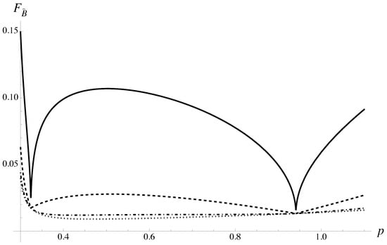
Figure 1. Amplitude B of the Schwinger model. Cost-functionals $F_{\overline{B}}(p,m)$, $k=3$, are shown for $m=1/2$ (solid line), $m=1$ (dashed line), $m=3/2$ (dashed–dotted line), and for $m=2$ (dotted line). See text for details.

2.2. Anomalous Dimension

The cusp anomalous dimension $\mathrm{\Omega }\left(g\right)$ of a light-like Wilson loop in the $n=4$ supersymmetric Yang–Mills theory depends only on the coupling g [26]. Only three non-trivial terms are known in the formal expansion as $g\to 0$. In the strong coupling limit $x\to \infty$, where $x=g^2$, $f\left(x\right)$ takes the form of a power law (2), with $B=2$ and $\beta =-1/2$.

The results of calculations for the amplitude B by different methods for $k=3$ are shown in Table 3.

Table 3. Amplitude B for anomalous dimension from various cost-functionals. The best result is shown in bold.

F, m	$\mathit{m}=1/2$	$\mathit{m}=1$	$\mathit{m}=3/2$	$\mathit{m}=2$	$\mathit{m}=5/2$
$F_B(p,m)$	2.01021	2.01759	2.01691	2.01321	2.00866
$F_{\overline{B}}(p,m)$	1.99854	2.00326	2.00316	2.001	1.99824
$F_C(p,m)$	2.0009	2.01759	2.03381	2.04874	2.06238
$F_{\overline{C}}(p,m)$	1.99337	2.00326	2.01506	2.02918	2.04659

Optimization according to $F_C(p,1/2)$, $k=3$ gives

$$B_1^{\ast }\left(p_{\mathrm{opt}}(1/2)\right)=1.76504,B_2^{\ast }\left(p_{\mathrm{opt}}(1/2)\right)=2.0001,B_3^{\ast }\left(p_{\mathrm{opt}}(1/2)\right)=2.0009,$$

corresponding to $p_{\mathrm{opt}}(1/2)=0.216427$. From the cost-functional (17) in the case of $k=3$, one finds $B\approx 2.0698$ [2].

The behavior of cost-functionals $F_C(p,m)$, $k=3$, is illustrated in Figure 2. In this case, catastrophic behavior is superseded by monotonous behavior, creating a global minimum.

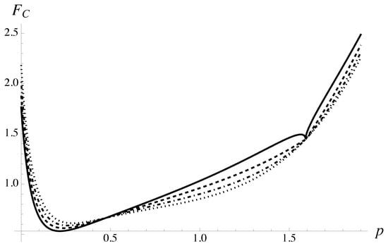
Figure 2. Critical amplitude for anomalous dimension. Cost-functionals $F_C(p,m)$ for $k=3$ are shown for $m=1/2$ (solid line), $m=1$ (dashed line), $m=3/2$ (dashed–dotted line), and for $m=2$ (dotted line). See text for details.

2.3. Bose Temperature Shift

Atomic interactions are known to stabilize the Bose gas. The shift $\mathsf{\Delta }{T}_c\equiv T_c-T_0$ in the Bose–Einstein condensation temperature $T_c$ of a non-ideal Bose system compared with the Bose–Einstein condensation temperature $T_0$ of the ideal uniform Bose gas [27,28] emerges and needs to be calculated.

The shift is quantified by the parameter $c_1$ in the following manner: $\mathsf{\Delta }{T}_c/T_0\simeq c_1\gamma ,$ for $\gamma \to 0$, where $\gamma$ is a gas parameter dependent on atomic scattering length and on gas density. In order to calculate $c_1$, it is expedient to first calculate an auxiliary function $c_1\left(g\right)$ [29,30,31]. The latter quantity is given as an expansion in terms of the effective coupling parameter g as $g\to 0$, in the fifth order. Eventually, $c_1$ corresponds to

$$B\equiv c_1=\underset{g\to \infty }{lim}{c}_1\left(g\right).$$

Monte Carlo simulations [32,33,34] give $B=1.3\pm 0.05$.

The results of calculations with different cost-functionals are presented in Table 4. The iterated roots employed in the course of calculations correspond to $k=4$.

Table 4. Bose temperature shift quantified by B from various cost-functionals ($k=4$). The best result is shown in bold.

F, m	$\mathit{m}=1/2$	$\mathit{m}=1$	$\mathit{m}=3/2$	$\mathit{m}=2$	$\mathit{m}=5/2$
$F_B(p,m)$	1.54664	1.54636	1.34636	1.29823	1.2792
$F_{\overline{B}}(p,m)$	1.3736	1.33524	1.30061	1.28194	1.2725
$F_C(p,m)$	1.30286	1.30284	1.28411	1.26857	1.26475
$F_{\overline{C}}(p,m)$	1.40249	1.33524	1.27921	1.26754	1.26463

Optimization according to $F_{\overline{B}}(p,3/2)$, $k=4$, gives

$$B_1^{\ast }\left(p_{\mathrm{opt}}(3/2)\right)=0.754224,B_2^{\ast }\left(p_{\mathrm{opt}}(3/2)\right)=0.986265,$$

$$B_3^{\ast }\left(p_{\mathrm{opt}}(3/2)\right)=1.23101,B_4^{\ast }\left(p_{\mathrm{opt}}(3/2)\right)=1.30061,$$

corresponding to $p_{\mathrm{opt}}(3/2)=0.759243$. The approximations converge monotonously.

From the cost-functional (17) in the case of $k=4$, one finds $B\approx 1.3829$ [2]. The behavior of cost-functionals $F_{\overline{B}}(p,m)$, $k=4$, is illustrated in Figure 3. In this case, catastrophic behavior is suppressed by monotonous behavior.

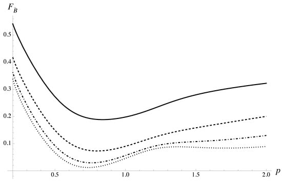
Figure 3. Amplitude B of Bose temperature shift. Cost-functionals $F_{\overline{B}}(p,m)$, $k=4$, are shown for $m=1/2$ (solid line), $m=1$ (dashed line), $m=3/2$ (dashed–dotted line), and for $m=2$ (dotted line).

For the $O\left(1\right)$ field theory, the corresponding expansion for the auxiliary function was obtained by Boris Kastening as well [29,30,31]. The Monte Carlo simulations give $B=1.09\pm 0.09$. The results of calculations by different methods are shown in Table 5.

Table 5. Condensation temperature of the $O\left(1\right)$ theory quantified by B for $k=4$. The best result is shown in bold.

F, m	$\mathit{m}=1/2$	$\mathit{m}=1$	$\mathit{m}=3/2$	$\mathit{m}=2$	$\mathit{m}=5/2$
$F_B(p,m)$	1.35492	1.33618	1.15371	1.11416	1.09643
$F_{\overline{B}}(p,m)$	1.14835	1.1341	1.11166	1.09697	1.08841
$F_C(p,m)$	1.12826	1.12826	1.10118	1.08474	1.0799
$F_{\overline{C}}(p,m)$	1.24346	1.13341	1.09368	1.08282	1.07949

Optimization according to $F_{\overline{B}}(p,5/2)$, $k=4$, gives

$$B_1^{\ast }\left(p_{\mathrm{opt}}(5/2)\right)=0.62853,B_2^{\ast }\left(p_{\mathrm{opt}}(5/2)\right)=0.834952,$$

$$B_3^{\ast }\left(p_{\mathrm{opt}}(5/2)\right)=1.05127,B_4^{\ast }\left(p_{\mathrm{opt}}(5/2)\right)=1.08841,$$

corresponding to $p_{\mathrm{opt}}(5/2)=0.750947$. The approximations converge monotonously. From the cost-functional (17), $B\approx 1.147$ is found.

For the $O\left(4\right)$ field theory, the fourth-order truncation was obtained by Kastening as well [29,30,31]. The Monte Carlo simulations give $B\equiv c_1=1.6\pm 0.1$. The results of calculations by different methods are shown in Table 6.

Table 6. Condensation temperature of the $O\left(4\right)$ theory quantified by B for k = 4. The best result is shown in bold.

F, m	$\mathit{m}=1/2$	$\mathit{m}=1$	$\mathit{m}=3/2$	$\mathit{m}=2$	$\mathit{m}=5/2$
$F_B(p,m)$	1.75812	1.75798	1.58793	1.53619	1.51972
$F_{\overline{B}}(p,m)$	1.65446	1.59461	1.54685	1.52429	1.51577
$F_C(p,m)$	1.51827	1.51818	1.51625	1.51105	1.51029
$F_{\overline{C}}(p,m)$	1.57274	1.57231	1.52068	1.51183	1.51044

Optimization according to $F_{\overline{B}}(p,1)$, $k=4$, gives

$$B_1^{\ast }\left(p_{\mathrm{opt}}\left(1\right)\right)=0.942784,B_2^{\ast }\left(p_{\mathrm{opt}}\left(1\right)\right)=1.19633,$$

$$B_3^{\ast }\left(p_{\mathrm{opt}}\left(1\right)\right)=1.46338,B_4^{\ast }\left(p_{\mathrm{opt}}\left(1\right)\right)=1.59461,$$

corresponding to $p_{\mathrm{opt}}\left(1\right)=0.773306$. The approximations converge monotonously. From the cost-functional (17), one finds $B\approx 1.6986$.

2.4. Two-Dimensional Polymer

The swelling factor $\mathrm{{\rm Y}}$ of the two-dimensional polymer was found perturbatively [35]. The asymptotic expansions of $\mathrm{{\rm Y}}$ are found in terms of the dimensionless coupling parameter g. The latter parameter measures the strength of the repulsive interaction between the segments of the polymer chain [35,36]. As $g\to 0$, the swelling factor can be represented as a fourth-order truncation of the type of expression (1). As $g\to \infty$, the swelling factor behaves as a power law of the type (2), with the exact index at infinity $\beta =1/2$ [37,38]. The amplitude B is of the order of unity.

The results of calculations by different methods are shown in Table 7.

Table 7. Amplitude B for two-dimensional polymer from various cost-functionals. The best result is shown in bold.

F, m	$\mathit{m}=1/2$	$\mathit{m}=1$	$\mathit{m}=3/2$	$\mathit{m}=2$	$\mathit{m}=5/2$
$F_B(p,m)$	0.973654	0.973611	0.976752	0.979166	0.979722
$F_{\overline{B}}(p,m)$	0.979785	0.979785	0.979786	0.979821	0.979822
$F_C(p,m)$	0.98221	0.98221	0.982088	0.980872	0.980058
$F_{\overline{C}}(p,m)$	0.949465	0.949464	0.982509	0.980698	0.980006

Optimization according to $F_{\overline{C}}(p,3/2)$, $k=4$, gives

$$B_1^{\ast }\left(p_{\mathrm{opt}}(3/2)\right)=0.950836,B_2^{\ast }\left(p_{\mathrm{opt}}(3/2)\right)=0.981627,$$

$$B_3^{\ast }\left(p_{\mathrm{opt}}(3/2)\right)=0.982509,B_4^{\ast }\left(p_{\mathrm{opt}}(3/2)\right)=0.932709,$$

corresponding to $p_{\mathrm{opt}}(3/2)=0.41739$. The approximations converge monotonously to the third member of the sequence $B_3^{\ast }\left(p_{\mathrm{opt}}(3/2)\right)$. From the cost-functional (17), $B\approx 0.9696$ is obtained.

2.5. Three-Dimensional Harmonic Trap

Quantum characteristics of Bose-condensed atoms in a spherically symmetric harmonic trap are modeled by the stationary nonlinear Schrödinger equation [27]. The ground-state energy E of the Bose condensate in such a trap is approximated for weak trappings $g\to 0$ by the fourth-order truncation. For quite strong trapping $g\to \infty$, the energy behaves as the power law (2), with the amplitude at infinity $B=5/4$, and the index $\beta =2/5$ [27].

The results of calculations for $k=4$ by different methods are shown in Table 8.

Table 8. Amplitude B of three-dimensional quantum trap for various cost-functionals. The best result is shown in bold.

F, m	$\mathit{m}=1/2$	$\mathit{m}=1$	$\mathit{m}=3/2$	$\mathit{m}=2$	$\mathit{m}=5/2$
$F_B(p,m)$	1.2845	1.2845	1.28303	1.28213	1.28203
$F_{\overline{B}}(p,m)$	1.27971	1.27971	1.27974	1.282	1.28202
$F_C(p,m)$	1.25848	1.27907	1.27915	1.27932	1.27936
$F_{\overline{C}}(p,m)$	1.26597	1.26629	1.27926	1.28132	1.28191

Optimization according to $F_C(p,1/2)$, $k=4$, gives

$$B_1^{\ast }\left(p_{\mathrm{opt}}(1/2)\right)=1.14295,B_2^{\ast }\left(p_{\mathrm{opt}}(1/2)\right)=1.20744,$$

$$B_3^{\ast }\left(p_{\mathrm{opt}}(1/2)\right)=1.24056,B_4^{\ast }\left(p_{\mathrm{opt}}(1/2)\right)=1.25848,$$

corresponding to $p_{\mathrm{opt}}(1/2)=1.66306$. The approximations converge monotonously to the last member of the sequence given by $B_4^{\ast }\left(p_{\mathrm{opt}}(1/2)\right)$. From the cost-functional (17), one finds $B\approx 1.2835$.

The behavior of cost-functionals $F_C(p,m)$, $k=4$, is illustrated in Figure 4. In this case, the catastrophic approach to the minimum is much more pronounced, while competing minima are almost suppressed.

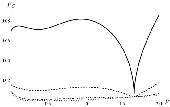
Figure 4. Amplitude B of trapped Bose condensate. Cost-functionals $F_C(p,m)$, $k=4$, are shown for $m=1/2$ (solid line), $m=1$ (dashed line), $m=3/2$ (dashed–dotted line), and for $m=2$ (dotted line).

2.6. Three-Dimensional Polymer

Just as in the example in Section 2.4, the expansion factor $\mathrm{{\rm Y}}\left(g\right)$ of a three-dimensional polymer can be represented as a truncated series in a single dimensionless interaction parameter g [35,36]. The expansion factor at small g can be presented as the sixth-order truncation. The strong coupling behavior of the expansion factor, as $g\to \infty$, is a power law with $B\approx 1.5309$ and $\beta \approx 0.3544$ [36]. The results of calculations by different methods are shown in Table 9.

Table 9. Amplitude B for three-dimensional polymer from various cost-functionals. The best result is shown in bold.

F, m	$\mathit{m}=1/2$	$\mathit{m}=1$	$\mathit{m}=3/2$	$\mathit{m}=2$	$\mathit{m}=5/2$
$F_B(p,m)$	1.52718	1.52718	1.53141	1.53225	1.53238
$F_{\overline{B}}(p,m)$	1.52883	1.52885	1.53126	1.53224	1.53238
$F_C(p,m)$	1.49426	1.49426	1.51318	1.5316	1.53214
$F_{\overline{C}}(p,m)$	1.49962	1.49969	1.51491	1.53142	1.5321

All methods presented in Table 9 give reasonable estimates for the amplitude. Optimization according to $F_{\overline{B}}(p,3/2)$, $k=6$, gives

$$B_1^{\ast }\left(p_{\mathrm{opt}}(3/2)\right)=1.47518,B_2^{\ast }\left(p_{\mathrm{opt}}(3/2)\right)=1.5088,B_3^{\ast }\left(p_{\mathrm{opt}}(3/2)\right)=1.52164,$$

$$B_4^{\ast }\left(p_{\mathrm{opt}}(3/2)\right)=1.52698,B_5^{\ast }\left(p_{\mathrm{opt}}(3/2)\right)=1.52975,B_6^{\ast }\left(p_{\mathrm{opt}}(3/2)\right)=1.53126,$$

corresponding to $p_{\mathrm{opt}}(3/2)=0.698365$. The approximations converge monotonously to the last member of the sequence given by $B_6^{\ast }\left(p_{\mathrm{opt}}(3/2)\right)$. From the cost-functional (17), one finds $B\approx 1.5272$ [2].

2.7. Pressure of a Two-Dimensional Membrane

For a two-dimensional membrane, it is essential to calculate its pressure. The wall stiffness is quantified by the dimensionless parameter g [39]. By means of perturbation theory, the expansion for the pressure at small g was found by Kastening in the sixth order of perturbation theory [39]. At infinite g, or in the so-called rigid-wall limit, Monte Carlo simulations [40] give the following estimate for the amplitude

$$B=p(\infty )=0.0798\pm 0.0003,$$

(18)

while the critical index at infinity is $\beta =2$. The results of calculations for $k=6$ by different methods are shown in Table 10.

Table 10. Amplitude B for two-dimensional membrane from various cost-functionals. The best result is shown in bold.

F, m	$\mathit{m}=1/2$	$\mathit{m}=1$	$\mathit{m}=3/2$	$\mathit{m}=2$	$\mathit{m}=5/2$
$F_B(p,m)$	0.0787295	0.078728	0.0786729	0.0771373	0.0740879
$F_{\overline{B}}(p,m)$	0.0798725	0.0798724	0.0794389	0.0754956	0.0738468
$F_C(p,m)$	0.0790725	0.0790731	0.0790115	0.0775616	0.074722
$F_{\overline{C}}(p,m)$	0.0800182	0.0800203	0.0796401	0.0758486	0.0739717

Optimization according to $F_{\overline{B}}(p,1)$, $k=6$, gives

$$B_1^{\ast }\left(p_{\mathrm{opt}}\left(1\right)\right)=0.0107064,B_2^{\ast }\left(p_{\mathrm{opt}}\left(1\right)\right)=0.0385531,B_3^{\ast }\left(p_{\mathrm{opt}}\left(1\right)\right)=0.0635931,$$

$$B_4^{\ast }\left(p_{\mathrm{opt}}\left(1\right)\right)=0.0773403,B_5^{\ast }\left(p_{\mathrm{opt}}\left(1\right)\right)=0.0798724,B_6^{\ast }\left(p_{\mathrm{opt}}\left(1\right)\right)=0.0397871,$$

corresponding to $p_{\mathrm{opt}}\left(1\right)=-0.848376$. The approximations converge monotonously to the fifth member of the sequence given by $B_5^{\ast }\left(p_{\mathrm{opt}}\left(1\right)\right)$.

From the cost-functional (17), one finds considerably inferior results, $B\approx 0.0598$ [2]. Also, the somewhat inferior results for $F_B(p,5/2)$, $F_{\overline{B}}(p,2)$, $F_{\overline{B}}(p,5/2)$, $F_{\overline{C}}(p,2)$, and $F_{\overline{C}}(p,5/2)$ are found from the minimal sensitivity condition (16).

2.8. One-Dimensional Bose Gas

The ground-state energy $E\left(g\right)$ of the one-dimensional Bose gas with contact interactions depends only on the dimensionless coupling parameter g [41]. The energy was found perturbatively in the eighth order as an expansion in terms of the variable x, where $g\equiv x^2$ [42]. In the limit of strong coupling, as $x\to \infty$, the exact result

$$E(\infty )=B={\displaystyle \frac{{\pi }^2}{3}}\approx 3.289868,$$

(19)

is due to Lewi Tonks [43] and Marvin Girardeau [44]. Formally, $\beta =-2$ is also set. In this case, one has to apply resummation to the inverse of the original truncations in order to avoid poles in the expression for amplitudes.

The results of calculations for $k=8$ by different techniques are shown in Table 11. In such a case, all approximations give quite suitable results independent of finer details of the cost-functional construction.

Table 11. Amplitude B for one-dimensional Bose gas from various cost-functionals. The best result is shown in bold.

F, m	$\mathit{m}=1/2$	$\mathit{m}=1$	$\mathit{m}=3/2$	$\mathit{m}=2$	$\mathit{m}=5/2$
$F_B(p,m)$	3.2092	3.2092	3.23367	3.2824	3.30576
$F_{\overline{B}}(p,m)$	3.17998	3.17998	3.24931	3.29358	3.3098
$F_C(p,m)$	3.19759	3.19759	3.22099	3.27213	3.30009
$F_{\overline{C}}(p,m)$	3.17582	3.17582	3.24027	3.28701	3.30648

Optimization according to $F_{\overline{C}}(p,2)$, $k=8$, gives

$$B_1^{\ast }\left(p_{\mathrm{opt}}\left(2\right)\right)=30.9749,B_2^{\ast }\left(p_{\mathrm{opt}}\left(2\right)\right)=8.71224,B_3^{\ast }\left(p_{\mathrm{opt}}\left(2\right)\right)=5.07523,$$

$$B_4^{\ast }\left(p_{\mathrm{opt}}\left(2\right)\right)=3.94466,B_5^{\ast }\left(p_{\mathrm{opt}}\left(2\right)\right)=3.45904,B_6^{\ast }\left(p_{\mathrm{opt}}\left(2\right)\right)=3.28701,$$

$$B_7^{\ast }\left(p_{\mathrm{opt}}\left(2\right)\right)=3.31854,B_8^{\ast }\left(p_{\mathrm{opt}}\left(2\right)\right)=3.67271,$$

corresponding to $p_{\mathrm{opt}}\left(2\right)=-0.480112$. The approximations converge monotonously to the sixth member of the sequence given by $B_6^{\ast }\left(p_{\mathrm{opt}}\left(2\right)\right)$. From the cost-functional (17), one finds considerably inferior results, $B\approx 4.507$ [2].

2.9. Gaussian Polymer: Debye–Hukel Function

The correlation function of the Gaussian polymer [37] is known in the following form:

$$\mathrm{\Phi }\left(x\right)={\displaystyle \frac{2}{x}}-{\displaystyle \frac{2(1-exp(-x\left)\right)}{x^2}},$$

(20)

and it is called the Debye–Hukel function. Consider for simplicity the inverse of the correlation function

$$\mathrm{\Psi }\left(x\right)={\displaystyle \frac{1}{\mathrm{\Phi }\left(x\right)}}.$$

For relatively small $x>0$, $\mathrm{\Psi }\left(x\right)$ can be expanded into a Taylor series with quite rapidly decaying by magnitude coefficients. As $x\to +\infty$, $\mathrm{\Psi }\left(x\right)$ behaves as a power law of the type (2), with $B=1/2$, $\beta =1$.

The results of calculations for $k=11$ are shown in Table 12. All methods give quite suitable results.

Table 12. Amplitude B for inverse Debye-Hukel function from various cost-functionals. The best result is shown in bold.

F, m	$\mathit{m}=1/2$	$\mathit{m}=1$	$\mathit{m}=3/2$	$\mathit{m}=2$	$\mathit{m}=5/2$
$F_B(p,m)$	0.49781	0.497819	0.497996	0.499976	0.500133
$F_{\overline{B}}(p,m)$	0.498088	0.498203	0.499687	0.500085	0.500152
$F_C(p,m)$	0.497811	0.497819	0.497913	0.498184	0.498346
$F_{\overline{C}}(p,m)$	0.498101	0.498203	0.49941	0.499974	0.500118

Optimization according to $F_B(p,2)$, $k=11$, gives

$$B_1^{\ast }\left(p_{\mathrm{opt}}\left(2\right)\right)=0.333333,B_2^{\ast }\left(p_{\mathrm{opt}}\left(2\right)\right)=0.44661,B_3^{\ast }\left(p_{\mathrm{opt}}\left(2\right)\right)=0.486048,$$

$$B_4^{\ast }\left(p_{\mathrm{opt}}\left(2\right)\right)=0.490291,B_5^{\ast }\left(p_{\mathrm{opt}}\left(2\right)\right)=0.489543,B_6^{\ast }\left(p_{\mathrm{opt}}\left(2\right)\right)=0.491477,$$

$$B_7^{\ast }\left(p_{\mathrm{opt}}\left(2\right)\right)=0.495745,B_8^{\ast }\left(p_{\mathrm{opt}}\left(2\right)\right)=0.496563,B_9^{\ast }\left(p_{\mathrm{opt}}\left(2\right)\right)=0.494589,$$

$$B_{10}^{\ast }\left(p_{\mathrm{opt}}\left(2\right)\right)=0.495819,B_{11}^{\ast }\left(p_{\mathrm{opt}}\left(2\right)\right)=0.499976,$$

corresponding to $p_{\mathrm{opt}}\left(2\right)=-0.669283$. The approximations converge almost monotonously with insignificantly weak oscillations to $B_{11}^{\ast }\left(p_{\mathrm{opt}}\left(2\right)\right)$. From the cost-functional (17), one finds considerably worse results, $B\approx 0.481018$. The latter result is close enough to “plain” Borel summation with iterated roots [1].

2.10. Schwinger Model: Energy Gap

The energy gaps $\mathsf{\Delta }\left(z\right)$ for the bound states of the Schwinger model can be presented as rather long asymptotic expansions at relatively small values of the parameter $z={(1/ga)}^4$, where a stands for lattice spacing and g is a coupling parameter [19]. In the continuous limit of $z\to \infty$, the gap for the scalar state behaves as a power law of the type of (2) [19],

$$\mathsf{\Delta }\left(z\right)\simeq B{z}^{\beta },$$

(21)

with $B=1.1284$, $\beta =1/4$.

The results of calculations for $k=11$ with different penalties are shown in Table 13.

Table 13. Amplitude B for energy gap of Schwinger model for various cost-functionals. The best result is shown in bold.

F, m	$\mathit{m}=1/2$	$\mathit{m}=1$	$\mathit{m}=3/2$	$\mathit{m}=2$	$\mathit{m}=5/2$
$F_B(p,m)$	1.16761	1.16141	1.16319	1.17642	1.2065
$F_{\overline{B}}(p,m)$	1.16438	1.16436	1.16488	1.17828	1.20823
$F_C(p,m)$	1.11717	1.11683	1.11729	1.12387	1.14931
$F_{\overline{C}}(p,m)$	1.11915	1.11885	1.11898	1.1258	1.15186

Optimization according to $F_{\overline{C}}(p,2)$ with $k=11$ gives

$$B_1^{\ast }\left(p_{\mathrm{opt}}\left(2\right)\right)=0.963112,B_2^{\ast }\left(p_{\mathrm{opt}}\left(2\right)\right)=1.02254,B_3^{\ast }\left(p_{\mathrm{opt}}\left(2\right)\right)=1.05607,$$

$$B_4^{\ast }\left(p_{\mathrm{opt}}\left(2\right)\right)=1.07608,B_5^{\ast }\left(p_{\mathrm{opt}}\left(2\right)\right)=1.09008,B_6^{\ast }\left(p_{\mathrm{opt}}\left(2\right)\right)=1.1,$$

$$B_7^{\ast }\left(p_{\mathrm{opt}}\left(2\right)\right)=1.10766,B_8^{\ast }\left(p_{\mathrm{opt}}\left(2\right)\right)=1.11363,B_9^{\ast }\left(p_{\mathrm{opt}}\left(2\right)\right)=1.11848,$$

$$B_{10}^{\ast }\left(p_{\mathrm{opt}}\left(2\right)\right)=1.12245,B_{11}^{\ast }\left(p_{\mathrm{opt}}\left(2\right)\right)=1.1258,$$

corresponding to $p_{\mathrm{opt}}\left(2\right)=1.41395$. The above approximations converge to $B_{11}^{\ast }\left(p_{\mathrm{opt}}\left(2\right)\right)$. From the cost-functional (17), one finds $B\approx 1.163$ [2]. The latter result is quite close to “plain” Borel summation with iterated roots [1].

2.11. Quantum Quartic Oscillator

The quantum anharmonic oscillator is described by the model Hamiltonian with a quartic term. The latter term is quantified through a positive anharmonicity parameter g [45]. Perturbation theory for the ground-state energy $E\left(g\right)$ produces a long expansion of the type (1), as shown in the seminal paper [45]. The coefficients $a_n$ are rapidly growing in magnitude with increasing n. The strong coupling limit case of $E\left(g\right)$ as $g\to \infty$ is given by the power law (2), with the critical amplitude $B=0.667986$ and index $\beta =1/3$.

The results of calculations for $k=11$ with different cost-functionals and corresponding penalties are shown in Table 14.

Table 14. Amplitude B for quantum quartic oscillator for various cost-functionals. The best result is shown in bold.

F, m	$\mathit{m}=1/2$	$\mathit{m}=1$	$\mathit{m}=3/2$	$\mathit{m}=2$	$\mathit{m}=5/2$
$F_B(p,m)$	0.676708	0.676708	0.679538	0.679324	0.679295
$F_{\overline{B}}(p,m)$	0.676281	0.676572	0.676803	0.679307	0.679292
$F_C(p,m)$	0.677082	0.678535	0.679164	0.679277	0.679289
$F_{\overline{C}}(p,m)$	0.678407	0.678891	0.679228	0.679284	0.679289

Optimization according to $F_{\overline{B}}(p,1/2)$, $k=11$, gives

$$B_1^{\ast }\left(p_{\mathrm{opt}}(1/2)\right)=0.74404,B_2^{\ast }\left(p_{\mathrm{opt}}(1/2)\right)=0.72319,B_3^{\ast }\left(p_{\mathrm{opt}}(1/2)\right)=0.705661,$$

$$B_4^{\ast }\left(p_{\mathrm{opt}}(1/2)\right)=0.693628,B_5^{\ast }\left(p_{\mathrm{opt}}(1/2)\right)=0.687914,B_6^{\ast }\left(p_{\mathrm{opt}}(1/2)\right)=0.685755,$$

$$B_7^{\ast }\left(p_{\mathrm{opt}}(1/2)\right)=0.684897,B_8^{\ast }\left(p_{\mathrm{opt}}(1/2)\right)=0.683117,B_9^{\ast }\left(p_{\mathrm{opt}}(1/2)\right)=0.68058,$$

$$B_{10}^{\ast }\left(p_{\mathrm{opt}}(1/2)\right)=0.67791,B_{11}^{\ast }\left(p_{\mathrm{opt}}(1/2)\right)=0.676281,$$

corresponding to $p_{\mathrm{opt}}(1/2)=0.917669$. The approximations converge numerically to $B_{11}^{\ast }\left(p_{\mathrm{opt}}(1/2)\right)$. From the cost-functional (17), one finds rather close results, $B\approx 0.6762$ [2]. The latter result is also quite close to “plain” Borel summation with iterated roots [1].

The best results, $B\approx 0.66936$, in the 10-th order of perturbation theory were found in Ref. [46] by means of fractional Borel summation. In the 11-th order, an even better estimate, $B\approx 0.667638$, can be found along the same lines.

3. Conclusions

The calculation of amplitudes emergent at quite large values of variable from the truncated series obtained for relatively small values of variable is performed by means of the cost-functional technique. In the five cases considered, the functionals, including essential singularities in the first derivatives, are found to perform better than functionals without it. One can conclude that there is definite value in considering such a catastrophic way of approaching optimum.

Most robust results are found with $F_{\overline{B}}(p,3/2)$, $F_{\overline{B}}(p,1)$, and $F_C(p,2)$. For better comparison, those results from Table 1, Table 2, Table 3, Table 4, Table 5, Table 6, Table 7, Table 8, Table 9, Table 10, Table 11, Table 12, Table 13 and Table 14 are compiled in Table 15. The functional $F_C(p,2)$ is a homogeneous function of the second order and, therefore, respects the scaling of all amplitudes with the same multiplicative factor. The other two cost functionals are non-homogenous and violate scaling. The cost-functional $F_{\overline{B}}(p,1)$ even allows for a catastrophic, “crash landing” approach to the optimum [3]. Cost-functional $F_{\overline{B}}(p,3/2)$ performs a little better than the other two compared to the tolerance level of $3\%$ in relative error.

Table 15. Robust performers. The best result compared to the exact B value shown is given in bold.

$\mathit{B},\mathit{F}$	${\mathit{F}}_{\overline{\mathit{B}}}(\mathit{p},1)$	${\mathit{F}}_{\overline{\mathit{B}}}(\mathit{p},3/2)$	${\mathit{F}}_{\mathit{C}}(\mathit{p},2)$	Exact B
Table 1	0.649474	0.63842	0.67106	0.6418
Table 2	0.649567	0.651297	0.667506	0.6418
Table 3	2.00326	2.00316	2.04874	2
Table 4	1.33524	1.30061	1.26857	1.3
Table 5	1.1341	1.11166	1.08474	1.09
Table 6	1.59461	1.54685	1.51105	1.6
Table 7	0.979785	0.979786	0.980872	1
Table 8	1.27971	1.27974	1.27932	5/4
Table 9	1.52885	1.53126	1.5316	1.5309
Table 10	0.0798724	0.0794389	0.0775616	0.0798
Table 11	3.17998	3.24931	3.27213	3.289868
Table 12	0.498202	0.499687	0.498184	1/2
Table 13	1.16436	1.16488	1.12387	1.1284
Table 14	0.676572	0.676803	0.679277	0.667986

Figure 1, Figure 2, Figure 3 and Figure 4 show various patterns of competition between “cusps” induced by penalty terms and “folds” originating from the rest of the terms. Is it possible to establish a more detailed correspondence with Thom’s theory of catastrophes [3]?

None of the approaches can consistently produce the best results for each and every problem. Most often, the best results are demonstrated by some other method than only the one mentioned just above. Being robust and being the best method simultaneously seems not attainable.

The approach applied here to the summation of asymptotic series in application to critical properties parallels current understanding of complex systems in their most general features. Certainly, the point is only about certain convergences of considerations from the two fields and not about deliberate developments.

In particular, criticality and power laws were considered in the limit of comparably large values of variables as emergent phenomena, since the underlying expansion at comparably small values of variables has rather different polynomial forms. Emergence and complexity are not equivalent but often related [47,48].

In addition, the study is concerned with cases when there are multiple solutions to the optimization problems, while the complex systems are understood to exist on the boundary or edge of chaos [49], when uncertainty in their behavior arises but predictability still exists [50]. Non-uniqueness of solutions may be seen as a manifestation of inherent chaos embedded into extrapolation with asymptotic truncated series, which could be overcome by imposing constraints through transformations, approximants, asymptotic conditions, and cost-functionals.

Finally, the iterated roots positioned at the core of the approach to extrapolation and criticality may be seen as self-referential constructs [51,52], with their shape remaining formally the same in each order and the parameters passed from the lower orders to higher orders or vice versa, as can be seen from Equation (4).

One can think that the parallels outlined above arise because asymptotic series are implicitly considered as an imprint left by the complex physical system and should be treated as such when a patently complicated problem of assigning meaningful values to asymptotic series at infinity is considered [53].

References

- Yukalov, V.I.; Gluzman, S. Resolving the problem of multiple control parameters in optimized Borel-type summation. J. Math. Chem. 2025, 63, 181–209. [Google Scholar] [CrossRef]
- Gluzman, S. Borel summation in a martingale-type collar. Axioms 2025, 14, 419. [Google Scholar] [CrossRef]
- Gilmore, R. Catastrophe Theory for Scientists and Engineers; Dover Publications: New York, NY, USA, 1993. [Google Scholar]
- Bender, C.M.; Orszag, S.A. Advanced Mathematical Methods for Scientists and Engineers: Asymptotic Methods and Perturbation Theory; Springer Science+Business Media: New York, NY, USA, 1999. [Google Scholar] [CrossRef]
- Andrianov, I.; Awrejcewicz, J. Asymptotic Methods for Engineers; CRC Press/Taylor & Francis Group: Boca Raton, FL, USA, 2024. [Google Scholar] [CrossRef]
- Bender, C.M.; Boettcher, S. Determination of f(∞) from the asymptotic series for f(x) about x=0. J. Math. Phys. 1994, 35, 1914–1921. [Google Scholar] [CrossRef]
- Gluzman, S. Iterative Borel summation with self-similar iterated roots. Symmetry 2022, 14, 2094. [Google Scholar] [CrossRef]
- Hardy, G.H. Divergent Series; Clarendon Press: Oxford, UK, 1949; Available online: https://archive.org/details/dli.ernet.285939 (accessed on 24 October 2025).
- Gluzman, S.; Yukalov, V.I. Self-similar extrapolation from weak to strong coupling. J. Math. Chem. 2010, 48, 883–913. [Google Scholar] [CrossRef]
- Gluzman, S. Critical permeability from resummation. Axioms 2024, 13, 547. [Google Scholar] [CrossRef]
- Yukalov, V.I. Theory of perturbations with a strong interaction. Moscow Univ. Phys. Bull. 1976, 31, 10–15. Available online: http://vmu.phys.msu.ru/abstract/1976/3/1976-17-3-270/ (accessed on 24 October 2025).
- Yukalov, V.I. Model of a hybrid crystal. Theor. Math. Phys. 1976, 28, 652–660. [Google Scholar] [CrossRef]
- Gisin, N. Indeterminism in physics and intuitionistic mathematics. Synthese 2021, 199, 13345–13371. [Google Scholar] [CrossRef]
- Tibshirani, R. Regression shrinkage and selection via the lasso. J. Roy. Stat. Soc. B 1996, 58, 267–288. [Google Scholar] [CrossRef]
- Tibshirani, R.; Friedman, J. A pliable lasso. J. Comput. Graph. Stat. 2020, 29, 215–225. [Google Scholar] [CrossRef] [PubMed]
- Tikhonov, A.N.; Arsenin, V.Y. Solution of Ill-Posed Problems; Winston & Sons: Washington, DC, USA, 1977. [Google Scholar]
- Tikhonov, A.N.; Leonov, A.S.; Yagola, A.G. Nonlinear Ill-Posed Problems; Chapman & Hall/CRC: London, UK, 1998. [Google Scholar]
- Yukalov, V.I.; Gluzman, S. Extrapolation of power series by self-similar Factor and root approximants. Int. J. Mod. Phys. B 1994, 18, 3027–3046. [Google Scholar] [CrossRef]
- Hamer, C.J.; Weihong, Z.; Oitmaa, J. Series expansions for the massive Schwinger model in Hamiltonian lattice theory. Phys. Rev. D 1997, 56, 55–67. [Google Scholar] [CrossRef]
- Carrol, A.; Kogut, J.; Sinclair, D.K.; Susskind, L. Lattice gauge theory calculations in 1+1 dimensions and the approach to the continuum limit. Phys. Rev. D 1976, 13, 2270–2277. [Google Scholar] [CrossRef]
- Vary, J.P.; Fields, T.J.; Pirner, H.J. Chiral perturbation theory in the Schwinger model. Phys. Rev. D 1996, 53, 7231–7238. [Google Scholar] [CrossRef]
- Adam, C. The Schwinger mass in the massive Schwinger model. Phys. Lett. B 1996, 382, 383–388. [Google Scholar] [CrossRef]
- Striganesh, P.; Hamer, C.J.; Bursill, R.J. A new finite-lattice study of the massive Schwinger model. Phys. Rev. D 2000, 62, 034508. [Google Scholar] [CrossRef]
- Coleman, S. More about the massive Schwinger model. Ann. Phys. 1976, 101, 239–267. [Google Scholar] [CrossRef]
- Hamer, C.J. Lattice model calculations for SU(2) Yang–Mills theory in 1+1 dimensions. Nucl. Phys. B 1977, 121, 159–175. [Google Scholar] [CrossRef]
- Banks, T.; Torres, T.J. Two point Padé approximants and duality. arXiv 2013, arXiv:1307.3689. [Google Scholar] [CrossRef]
- Courteille, P.W.; Bagnato, V.S.; Yukalov, V.I. Bose–Einstein condensation of trapped atomic gases. Laser Phys. 2001, 11, 659–800. [Google Scholar] [CrossRef]
- Yukalov, V.I.; Yukalova, E.P. Bose–Einstein condensation temperature of weakly interacting atoms. Laser Phys. Lett. 2017, 14, 073001. [Google Scholar] [CrossRef]
- Kastening, B. Shift of BEC temperature of homogenous weakly interacting Bose gas. Laser Phys. 2004, 14, 586–590. [Google Scholar]
- Kastening, B. Bose–Einstein condensation temperature of a homogenous weakly interacting Bose gas in variational perturbation theory through seven loops. Phys. Rev. A 2004, 69, 043613. [Google Scholar] [CrossRef]
- Kastening, B. Nonuniversal critical quantities from variational perturbation theory and their application to the Bose–Einstein condensation temperature shift. Phys. Rev. A 2004, 70, 043621. [Google Scholar] [CrossRef]
- Arnold, P.; Moore, G. BEC transition temperature of a dilute homogeneous imperfect Bose gas. Phys. Rev. Lett. 2001, 87, 120401. [Google Scholar] [CrossRef] [PubMed]
- Arnold, P.; Moore, G.D. Monte Carlo simulation of O(2)ϕ4 field theory in three dimensions. Phys. Rev. E 2001, 64, 066113. [Google Scholar] [CrossRef]
- Nho, K.; Landau, D.P. Bose–Einstein condensation temperature of a homogeneous weakly interacting Bose gas: Path integral Monte Carlo study. Phys. Rev. A 2004, 70, 053614. [Google Scholar] [CrossRef]
- Muthukumar, M.; Nickel, B.G. Perturbation theory for a polymer chain with excluded volume interaction. J. Chem. Phys. 1984, 80, 5839–5850. [Google Scholar] [CrossRef]
- Muthukumar, M.; Nickel, B.G. Expansion of a polymer chain with excluded volume interaction. J. Chem. Phys. 1987, 86, 460–476. [Google Scholar] [CrossRef]
- Grosberg, A.Y.; Khokhlov, A.R. Statistical Physics of Macromolecules; AIP Press: Woodbury, NY, USA, 1994. [Google Scholar]
- Pelissetto, A.; Vicari, E. Critical phenomena and renormalization-group theory. Phys. Rep. 2002, 368, 549–727. [Google Scholar] [CrossRef]
- Kastening, B. Fluctuation pressure of a fluid membrane between walls through six loops. Phys. Rev. E 2006, 73, 011101. [Google Scholar] [CrossRef] [PubMed]
- Gompper, G.; Kroll, D.M. Steric interactions in multimembrane systems: A Monte Carlo study. Eur. Phys. Lett. 1989, 9, 59–64. [Google Scholar] [CrossRef]
- Lieb, E.H.; Liniger, W. Exact analysis of an interacting Bose gas: The general solution and the ground state. Phys. Rev. 1963, 130, 1605–1616. [Google Scholar] [CrossRef]
- Ristivojevic, Z. Conjectures about the ground-state energy of the Lieb–Liniger model at weak repulsion. Phys. Rev. B 2019, 100, 081110. [Google Scholar] [CrossRef]
- Tonks, L. The complete equation of state of one, two and three-dimensional gases of hard elastic spheres. Phys. Rev. 1936, 50, 955–963. [Google Scholar] [CrossRef]
- Girardeau, M. Relationship between systems of impenetrable bosons and fermions in one dimension. J. Math. Phys. 1960, 1, 516–523. [Google Scholar] [CrossRef]
- Hioe, F.T.; McMillen, D.; Montroll, E.W. Quantum theory of anharmonic oscillators: Energy levels of a single and a pair of coupled oscillators with quartic coupling. Phys. Rep. 1978, 43, 305–335. [Google Scholar] [CrossRef]
- Gluzman, S. Borel transform and scale-invariant fractional derivatives united. Symmetry 2023, 15, 1266. [Google Scholar] [CrossRef]
- Albeverio, S.; Mastrogiacomo, E.; Gianin, E.R.; Ugolini, S. (Eds.) Complexity and Emergence. Lake Como School of Advanced Studies, Italy, July 22–27, 2018; Springer Nature Switzerland AG: Cham, Switzerland, 2022. [Google Scholar] [CrossRef]
- Fuentes, M. Complexity, Emergence and the Evolution of Scientific Theories: Towards a Predictive Epistemology; Springer Nature Switzerland AG: Cham, Switzerland, 2025. [Google Scholar] [CrossRef]
- Crutchfield, J.P.; Young, K. Computation at the onset of chaos. In Entropy, Complexity, and Physics of Information. The Proceedings of the 1988 Workshop on Complexity, Entropy, and the Physics of Information Held May–June, 1989, In Santa Fe, New Mexico; Zurek, W.H., Ed.; Addison-Wesley Publishing Company: Redwood City, CA, USA, 1990; pp. 223–269. Available online: https://www.scribd.com/document/724978070/Complexity-Entropy-and-the-Physics-of-Information-The-proceedings-of-the-1988-workshop-on-Complexity-Entropy-and-the-Physics-of-Information (accessed on 24 October 2025).
- Baym, M.; Hübler, A.W. Conserved quantities and adaptation to the edge of chaos. Phys. Rev. E. 2006, 73, 056210. [Google Scholar] [CrossRef]
- Youvan, D.C. Self-Referential Emergent Systems Can Exist as Self-Sustaining Loops Without Reliance on Hierarchical Substructures. 2 January 2025. [CrossRef]
- Hempel, S.; Pineda, R.; Smith, E. Self-reference as a principal indicator of complexity. Procedia Comput. Sci. 2011, 6, 22–27. [Google Scholar] [CrossRef]
- Andrianov, I.V.; Khajiyeva, L.A. 60 years of asymptotology—Preliminary results. Or “in Memoriam?”. In Dynamics of Discrete and Continuum Structures and Media, Advanced Structured Materials; Altenbach, B.H., Eremeyev, V.A., Eds.; Nature Switzerland AG: Cham, Switzerland, 2025; pp. 43–57. [Google Scholar] [CrossRef]
Disclaimer/Publisher’s Note: The statements, opinions and data contained in all publications are solely those of the individual author(s) and contributor(s) and not of MDPI and/or the editor(s). MDPI and/or the editor(s) disclaim responsibility for any injury to people or property resulting from any ideas, methods, instructions or products referred to in the content. |
© 2025 by the author. Licensee MDPI, Basel, Switzerland. This article is an open access article distributed under the terms and conditions of the Creative Commons Attribution (CC BY) license (https://creativecommons.org/licenses/by/4.0/).